Giant Molecular Clouds in M64

Abstract

We investigate the properties of Giant Molecular Clouds (GMCs) in the molecule-rich galaxy M64 (NGC 4826). In M64, the mean surface density of molecular gas is $2N(\mbox{H}_{2})\sim 10^{22}$ over a 2 kpc region, equal to the surface densities of individual GMCs in the Milky Way. We observed the $J=1\to 0$ transitions of CO, ${}^{13}\mbox{CO}$, and HCN. The line ratio $W_{\mathrm{CO}}/W_{\mathrm{13CO}}$ for $200\mbox{ pc}<R_{gal}<800\mbox{ pc}$ is comparable to that found in the Milky Way and increases significantly outside this region, in part due to a large contribution to the CO emission from diffuse gas, which composes 25% of the molecular mass in the galaxy. We developed a modified CLUMPFIND algorithm to decompose the ${}^{13}\mbox{CO}$ emission into 25 resolved clouds. The clouds have a luminosity–linewidth relationship $L\propto\Delta V^{2.2\pm 0.4}$, substantially different from the Milky Way trend reported by Solomon et al. (1987): $L\propto\Delta V^{5}$. Similarly, the clouds have a linewidth–size relationship of $\Delta V\propto R_{e}^{1.0\pm 0.3}$ compared to $\Delta V\propto R_{e}^{0.5}$ in the Milky Way. Estimates of the kinetic and binding energies of the clouds suggest that the clouds are self-gravitating and significantly overpressured with respect to the remainder of the ISM in M64. The ${}^{13}\mbox{CO}$-to-H₂ conversion factor is comparable to what is seen in the Galaxy. The M64 clouds have a mean surface density at least 2.5 times larger than observed in Local Group GMCs, and the surface density is not independent of mass as it is in the Local Group: $\Sigma_{\mathrm{H2}}\propto M^{0.7\pm 0.2}$. The clouds are correlated with the recombination emission from the galaxy, implying that they are star forming; the rate is comparable to that in other galaxies despite the increased densities of the clouds. The gas-to-dust ratio is similar to the Galactic value but the low extinction in the visual band requires that the molecular gas be clumpy on small scales. We note that the internal pressures of clouds in several galaxies scales with the external pressure exerted on the clouds by the ambient ISM: $P_{int}\propto P_{ext}^{0.75\pm 0.05}$. We attribute the differences between M64 molecular cloud and those in the Local Group to the high ambient pressures and large molecular gas content found in M64.

1. Introduction

Over 80% molecular gas in the Milky Way is found in Giant Molecular Clouds (GMCs) with masses $10^{3}~{}M_{\odot}<M_{GMC}<10^{6.5}~{}M_{\odot}$ and sizes between 2 and 100 pc. They have a column density of $2N(\mbox{H}_{2})\sim 10^{22}~{}\mbox{cm}^{-2}$, independent of mass (Blitz, 1993). Observations of molecular gas across the Local Group have found that most of the molecular gas in these systems is also found in GMCs with properties similar to those in the disk of the Milky Way (Mizuno et al., 2001; Engargiola et al., 2003; Young, 2000; Bolatto et al., 2003). Beyond the Local Group, observers find several galaxies where the typical molecular column density through the galactic disks is $>10^{22}\mbox{ cm}^{-2}$ (Helfer et al., 2003) on kiloparsec scales implying that the ISM is overwhelmingly molecular, since the column densities of atomic gas are only rarely seen to exceed $10^{21}$ cm^-2. Since this is larger than the typical column density through a single GMC in the Local Group, the molecular ISM must be qualitatively different in these galaxies. Do the molecular clouds in these galaxies blend together into a continuous sea of molecular gas or are there discrete clouds of molecular gas that are denser than Local Group GMCs? Moreover, what are the star forming structures in this molecular gas? In the Local Group, star formation is predominantly found in GMCs, but if there are no discrete clouds in this molecular gas, do stars form uniformly throughout the galaxy from stellar mass clumps in the sea of gas? If there are GMCs but they are smaller and denser than Local Group clouds, is the star formation efficiency enhanced? In order to answer these questions, we have conducted a study of the molecule-rich galaxy M64 (NGC 4826) at high resolution to search for GMC analogues in a molecule-rich environment.

M64 is a good target for such a study because it has a mean column density across the central 2 kpc of the galaxy of $2N(\mbox{H}_{2})=10^{22}~{}\mbox{cm}^{-2}$, making it an intermediate case between the Local Group and starburst galaxies. The galaxy is one of the closest molecule rich galaxies (4.1 Mpc, Tully, 1988). A merger with a small, gas-rich galaxy roughly 1 Gyr ago is thought to be responsible for the relatively large molecular gas content for its early Hubble type (SA) (Braun et al., 1994, B94). The 3$\farcs$5 resolution obtained with the BIMA millimeter interferometer projects to 75 pc, which would be sufficient to resolve the largest molecular clouds in the Milky Way disk at the distance of M64. Two other recent studies examine properties of molecular emission in the nucleus of M64. Meier (2002, M02) conducted a study of the nuclear region using the OVRO millimeter array in the 3 mm transitions of CO, ${}^{13}\mbox{CO}$, and C¹⁸O. The primary beam at OVRO has a FWHM of 65^′′ which samples gas to $R_{gal}=600$ pc along the major axis and the map has a $5^{\prime\prime}$ synthesized beam. These observations were principally used to determine the bulk properties of the molecular gas using LVG analyses. García-Burillo et al. (2003, hereafter NUGA) also conducted an extensive analysis of the molecular gas in the nuclear region using the IRAM Plateau de Bure interferometer (PdBI) in the CO$(2\to 1)$ and the CO$(1\to 0)$ transitions. With the 42^′′ primary beam, the PdBI observations cover the galaxy to $R_{gal}=420$ pc for the $(1\to 0)$ transition with a $2.5^{\prime\prime}$ resolution. The NUGA project focused interpretation of their data on the mechanisms by which the central AGN could be fed. Our search for molecular clouds in M64 is complementary to the aims of both M02 and NUGA. With a 105^′′ primary beam and $3.5^{\prime\prime}$, our BIMA study maps the galaxy to the edge of the molecular disk at $R_{gal}\gtrsim 1000$ pc permitting a more thorough study of the molecular gas. In addition, this study includes zero-spacing observations of CO and ${}^{13}\mbox{CO}$ which are essential in searching for low surface brightness gas among the clouds. In this paper, we report on our observations (§2), examine the dynamics of the molecular disk (§3.1) and variations in the isotopic line ratios (§3.2), decompose the blended emission into cloud candidates and argue that these candidates represent the high density analogues of Local Group GMCs (§4).

2. Observations

2.1. Molecular Line Observations

We observed M64 using the BIMA array (Welch et al., 1996) in three tracers of molecular gas: CO$(1\to 0)$, ${}^{13}\mbox{CO}$$(1\to 0)$ and HCN$(1\to 0)$. We utilized data from the B, C and D arrays, including medium-resolution (C array) and zero-spacing (UASO 12-m) observations made in the BIMA Survey of Nearby Galaxies (SONG, Helfer et al., 2003). The combined observations resulted in a synthesized beam of $3.5^{\prime\prime}$ which projects to a linear scale of 75 pc. Details for the individual observations appear in Table 1. We calibrated the visibility data using the same techniques as employed in SONG. The visibility data were inverted using natural weighting to maximize signal-to-noise ratios. The high resolution CO observations had slightly different pointing centers with respect to the low resolution and zero-spacing data, requiring inversion to the image domain of the high and low resolution data separately. We then combined these CO maps using the linear combination method (Stanimirovic et al., 1999; Helfer et al., 2003). Images were then cleaned using a hybrid Högbom / Clark / SDI algorithm with the residuals of the cleaned components added back in to avoid any flux loss. To check for possible contamination by continuum emission from the AGN, we imaged the LSB data from ${}^{13}\mbox{CO}$ and HCN. The lack of sources in the resulting maps places a 3$\sigma$ point source sensitivity of 3.4 mJy at 85 GHz for objects in the galaxy and a 3.2 mJy limit at 106 GHz.

Table 1Properties of BIMA Array Observations

Tracer	Array	Length	$\langle T_{sys}\rangle$	Beam Size	$\sigma_{rms}$
		[hours]	[K]	[′′]	[Jy bm-1 km s-1]
12CO$(1\to 0)$	B	11 h 20 m	610	$4.6\times 3.6$	0.24
	C	10 h 57 m	417
13CO$(1\to 0)$	B	22 h 35 m	264	$3.3\times 2.6$	0.11
	C	12 h 05 m	430
	D	3 h 35 m	305
HCN$(1\to 0)$	B	16 h 01 m	198	$4.0\times 3.4$	0.037
	C	7 h 47 m	221
	D	3 h 58 m	194

Although M64 has been partially mapped with the IRAM 30-m telescope (Casoli & Gerin, 1993), the data are no longer available in an electronic format (F. Casoli, private communication). To provide a fully-sampled ${}^{13}\mbox{CO}$ map, we observed the galaxy with the FCRAO 14-m telescope. We observed 7 points arranged in a hexagonal pattern in order to obtain a Nyquist-sampled map and recover all spatial frequencies. Observations of SiO maser stars through the night were used to check the pointing solution of the telescope. We observed the galaxy by alternately pointing at the galaxy with two different pixels in the SEQUOIA 32-pixel receiver. We used the time that each pixel was pointed at blank sky as the reference position for that pixel. Vane calibration was used to set the flux scale. We used two back ends in parallel: the Quabbin Extragalactic Filterbank (QEF), which provided 320 MHz of spectral coverage in 64 5-MHz channels (864 km s^-1 divided into 13.5 km s^-1 channels), and the Focal Plane Array Autocorrelation Spectrometer (FAAS), which provided 80 MHz of spectral coverage with 0.3125 MHz channels (216 km s^-1 divided into 0.84 km s^-1 channels). Unfortunately, the velocity range of 216 km s^-1 provided by the FAAS correlator is insufficient to cover the entire galaxy and the velocity resolution of the QEF was too coarse to merge with the interferometer data. Therefore, we had to observe the galaxy with two separate velocity configurations which measured the approaching and receding halves of the galaxy separately. We used the QEF data to establish the common scaling between the two velocity configurations. Since the FAAS and QEF follow the same amplifier chain, smoothing FAAS data to the QEF resolution should result in the same spectrum. To stitch together the two sets of FAAS data, we subtracted a linear baseline from the QEF data and used the resulting spectrum as a model of signal emission in the FAAS data. By accounting for the expected signal using the QEF data, a linear baseline could be removed from each of the FAAS spectra separately and spectra from the two configurations could be merged. An example of this appears in Figure 1. Typically, the spectra had a noise level of 12 mK in a 4.25 km s^-1 channel after correcting for a main beam efficiency of 0.5 at 110 GHz. As a check, we smoothed the final FAAS spectrum to the resolution of the QEF data and found there were only small variations resulting from higher order baselines in the data sets.

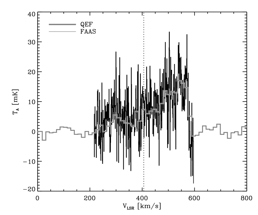
Figure 1.— Example of resulting spectrum from stitching procedure. This spectrum is taken at $\alpha_{2000}=12^{\mathrm{h}}56^{\mathrm{m}}42\fs 7,\delta_{2000}=+21^{\circ}41^{\prime}18\farcs 5$ spectra are merged around the LSR velocity of the galaxy, shown with the dotted line at 406 km s^-1. This shows the general success of producing a combined high-resolution spectrum from different velocity configurations.

We merged the zero-spacing information with the ${}^{13}\mbox{CO}$ interferometer data using the Linear Combination technique (Stanimirovic et al., 1999; Helfer et al., 2003). The merged dataset was deconvolved using a CLEAN algorithm which terminated at the 1.5$\sigma_{rms}$ level of the data. The combined dataset contains $94\pm 7\%$ of the single dish flux. Finally, we regridded the CO and HCN images to match the spatial and velocity scale of the ${}^{13}\mbox{CO}$ data to facilitate pixel-to-pixel comparison, resulting in a final channel width of 4.25 km s^-1 in all maps.

Table 2Flux Recovery for BIMA Observations

Tracer	Flux	SD Flux	Frac.	Completeness Lmt.
	Jy km s-1	Jy km s-1	Recovered	Jy km s-1
CO	$1678\pm 23$	$1845\pm 217$	$91\pm 12$%	1.06
${}^{13}\mbox{CO}$	$160\pm 6$	$230\pm 10$	$70\pm 6$%	0.35
HCN	$35\pm 3$	$36.5\pm 5.6$	$96\pm 18$%	0.20

2.2. Recombination Line Images

To obtain recombination line emission images, we downloaded HST images of the galaxy in Pa$\alpha$ (F187N), $H$-band continuum (F160W), H$\alpha$ (F656N) and $V$-band continuum (F547M) from the HST data archive. The Pa$\alpha$ image was presented originally by Böker et al. (1999). We followed the reduction steps presented in that work including removal of the ‘pedestal effect’ in the NIC3 camera. However, we adopted a different optimal scaling between the F160W continuum image ($W_{ij}$) and the F187N line image ($N_{ij}$) for continuum subtraction. We minimize a goodness-of-fit parameter $G(m)=\sum_{ij}|(N_{ij}-mW_{ij})/\sigma_{ij}|^{p}$ with respect to the scaling $m$, where $\sigma_{ij}$ is the noise associated with each pixel and the power $p$ is determined by

$$p=\left\{\begin{array}[]{cl}0.5,&N_{ij}\geq mW_{ij}\\ 6,&N_{ij}<mW_{ij}.\end{array}\right.$$

This construction preferentially fits those points in the narrow band image that are free from Pa$\alpha$ emission. For the NICMOS data, $m=0.0418$. This method implicitly assumes that the color of the continuum does not vary across the map.

The H$\alpha$ images have not been published, and were observed under HST GO Proposal #8591 (Richstone, D.). We used a similar procedure to that of the Pa$\alpha$ analysis to extract an image containing only H$\alpha$ line flux from the archival data. The principal differences were that we used median filtering among an array of images to eliminate cosmic rays. We used a F547M image of the galaxy for the continuum image and the F656N image containing the line flux. The optimal scaling between these two images is, on average, $m=0.304$ though data from each chip of the WFPC2 were treated separately.

3. Analysis of the Molecular Line Maps

In Figures 2 to 4, we present velocity-integrated maps of the molecular disk in M64. The data have been masked to highlight the structure of the emission in the three maps. Since all three data sets have the same coordinate axes, a single mask is generated common to all three data sets. An element is included in the mask if it has detectable emission in CO. For the CO data, the masking process begins by searching for all positions with emission ($I$) greater than 4 times the rms value of the noise ($\sigma_{rms}$) in two adjacent velocity channels. These regions are then expanded to include all pixels with $I\geq 2\sigma_{rms}$ that are connected in position or velocity space by $\geq 2\sigma_{rms}$ detections to the joint $4\sigma_{rms}$ detection “core” following the method used in Engargiola et al. (2003). For comparison, we have plotted an integrated intensity image using a 2$\sigma_{rms}$ clip in the right-hand panel of Figure 2. The mask generated from the CO is then applied to the ${}^{13}\mbox{CO}$ and HCN emission. Using a common mask among the different tracers facilitates direct comparison of the morphology of the molecular emission. We use this process since emission from rare tracers will be located in the regions of the datacube where there is emission from the more common tracers. Because of this assumption, the masked maps have complex statistical properties since the CO map contains only positive emission while the ${}^{13}\mbox{CO}$ and HCN emission include noise in the data. Nonetheless, the masking process highlights faint HCN emission in the disk of the galaxy which is difficult to detect by analyzing the HCN emission alone (Figure 4). These faint features align with the strong CO features seen in Figures 2 and 3. We used Monte Carlo simulations to establish point source completeness limits with this masking algorithm for emission with a velocity FWHM of 2 channels. The quoted limits in Table 2 are the threshold for a point source to be recovered in 90% of the Monte Carlo trials. We use this masking process to examine the structure of the emission and for the rotation curve but use simpler methods for line ratio studies and cloud decomposition.

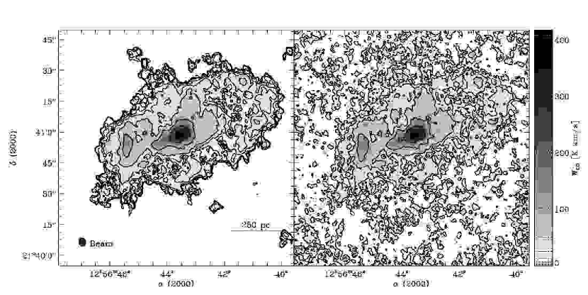
Figure 2.— Masked integrated emission map of M64 in ¹²CO$(1\to 0)$ for two different masking methods. The masking method used in the paper (left panel) is compared to a mask generated by clipping the emission above $2\sigma_{rms}$ (right panel). Comparing the two methods highlights the ability for the adopted method to recover low surface brightness emission. In the left panel, contours are $2^{k}\sigma_{rms}$ for $k\geq 0$ and in the right panel, contours are $2^{j}\sigma_{rms}$ for $j\geq 3$. . The levels of the contours relative to the grayscale are indicated in the colorbar by dotted lines.

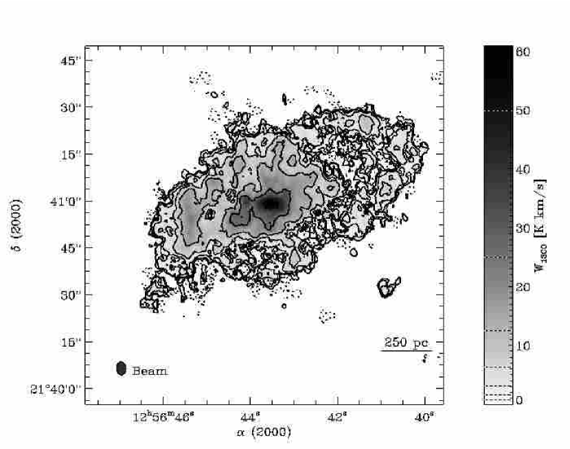
Figure 3.— Masked integrated emission map of M64 in ¹³CO$(1\to 0)$. The contours are $-2\sigma_{rms}$, $-1\sigma_{rms}$ (dotted) and $2^{k}\sigma_{rms}$ for $k\geq 0$ (solid). The levels of the contours relative to the grayscale are indicated in the colorbar by dotted lines. The emission appears significantly more clumpy than the ¹²CO emission despite similar $UV$ coverage.

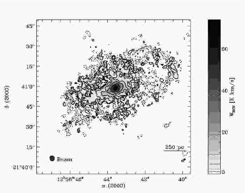
Figure 4.— Masked integrated emission map of M64 in HCN$(1-0)$. The contours are $-2\sigma_{rms}$, $-1\sigma_{rms}$ (dotted) and $2^{k}\sigma_{rms}$ for $k\geq 0$ (solid). The levels of the contours relative to the grayscale are indicated in the colorbar by dotted lines. The emission is strongly peaked in the nuclear region of the galaxy, but the masking procedure highlights faint emission, particularly in the NE half of the disk.

The three maps share several common features. The emission is strongly peaked at the center of the galaxy with a surrounding disk. The NE half of the disk shows stronger emission than the SW half. The molecular emission in the NE half of the galaxy aligns with the prominent dust lane that earns the galaxy’s nickname of the ‘Evil Eye;’ however, these observations show that there is significant molecular gas in the SW of the galaxy as well. The disk appears to cut off sharply at a galactocentric radius of $R_{gal}=1000$ pc. To quantify this, we plot the azimuthally averaged surface brightness distributions in Figure 5. The azimuthal average shows a significant cutoff at $R_{gal}=925\pm 25$ pc in the CO emission, well above the $3\sigma_{rms}$ noise level of the observations. A similar cutoff is also seen in the ${}^{13}\mbox{CO}$ emission and likely exists in the HCN emission but is below our significance threshold.

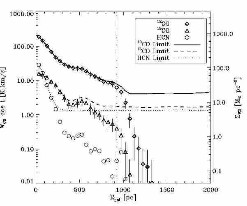
Figure 5.— Azimuthally averaged surface brightness for molecular tracers. The averages were taken in 50 pc bins. The error bars represent 1$\sigma$ errors and the lines indicating upper-limits represent the profile that would be observed if the blank pixels contained emission at the $3\sigma_{rms}$ level, a very conservative upper limit. The averages have been scaled by $\cos i=\cos 56^{\circ}$ to reflect face on values. The CO emission shows a marked truncation at $R_{gal}=925\pm 25$ pc, indicated by the vertical dotted line.

3.1. The Rotation Curve of M64

M64 is peculiar because the outer H I disk ($R_{gal}>2$ kpc) is counterrotating with respect to the inner H I and stellar disks. Studies by Braun et al. (1994) and Rix et al. (1995) suggest that the outer disk is result of a retrograde merger with a small galaxy. They propose that interaction between the counterrotating gas disk and the prograde stellar+gas disk dissipates significant angular momentum, fueling infall to the central disk which accounts for the high values of the surface mass density of neutral gas (Rix et al., 1995; Rubin, 1994). However, the gas in the central region of the galaxy ($R_{gal}\lesssim 1$ kpc) appears to be in a normal, rotating disk which is decoupled from the peculiar dynamics of the outer galaxy. The outer edge of the molecular disk occurs at the interface between the well-organized inner disk and the infalling ionized gas in the in region $1000\mbox{ pc}<R_{gal}<1500\mbox{ pc}$.

Since these are the first millimeter observations to cover the entirety of the molecular gas disk, we examined the dynamics of the inner region of the galaxy. We generated velocity fields from the masked emission for each of the three tracers. We analyzed the velocity fields using the tilted-ring algorithm first presented by Begeman (1989) to generate a rotation curve as implemented in the NEMO stellar dynamics toolkit (Teuben, 1995). We used literature values for initial estimates of the circular rotation speed, position angle, inclination, systemic velocity and dynamical center (B94, NUGA). We then iteratively fit for these parameters until a convergent model was determined following the procedure described in Wong et al. (2004). The derived parameters of the disk do not vary significantly for the molecular emission within $40^{\prime\prime}$ of the galactic center, so we forced the inclination, position, systemic velocity, and position angle of the rings to be equal in order to improve the estimate of the dynamical properties. The dynamical center of the galaxy is at $\alpha_{2000}=12^{\mbox{\scriptsize h}}\ 56^{\mbox{\scriptsize m}}\ 43\fs 6$ and $\delta_{2000}=21\arcdeg\ 40\arcmin\ 57\farcs 7$ with a systemic velocity of $V_{sys}=411\pm 1\mbox{ km s}^{-1}$. The disk of the galaxy has a position angle of $-67\arcdeg\pm 3\arcdeg$ and an inclination $i=59\arcdeg\pm 2\arcdeg$ averaged over $R_{gal}<40^{\prime\prime}$ using 4^′′ bins including corrections in the quoted errors for beam smearing and oversampling. These dynamical properties agree well with those adopted by other authors. The peak of the molecular emission is slightly offset ($1^{\prime\prime}$) from the dynamical center of the galaxy, as is found in many disk galaxies (Helfer et al., 2003).

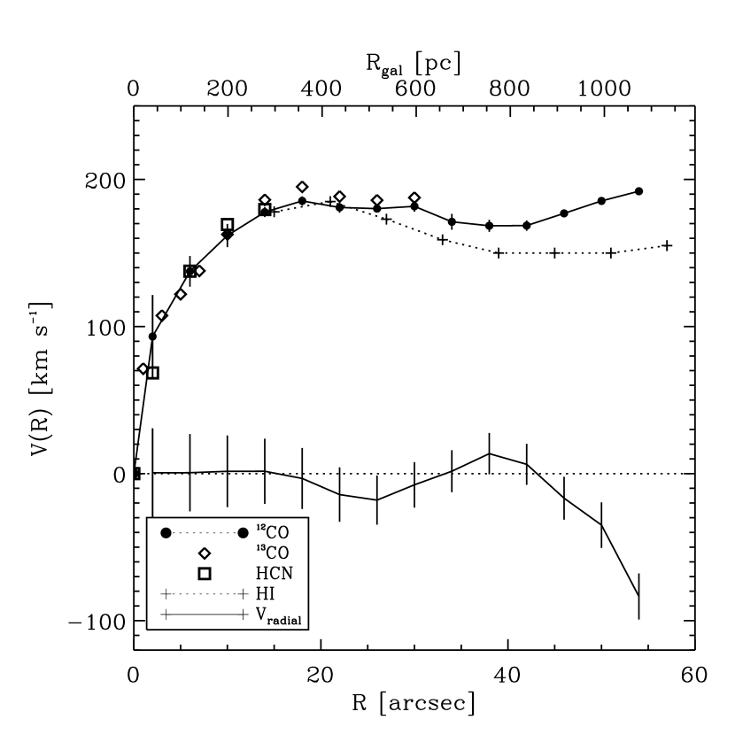
Figure 6.— Rotation curve of M64. The data agree well until the small numbers of points that show ¹³CO emission lead to poor fits in the outer section of the galaxy. Typical errors in the derived rotation velocities vary between 0.5 and 10 km s^-1 and $1\sigma$ error bars are plotted for the ¹²CO points. We also plot the radial velocity derived from an axisymmetric inflow/outflow model.

The rotation curve of the galaxy is shown in Figure 6 for each of the three tracers and the H I (from B94). The rotation curves agree well for the three tracers in the inner portions of the galaxy. At large radii, the H I rotation curve differs from that of the molecular gas. This may be a physical effect arising from infalling material interacting with the molecular disk. Radial motions are seen in the atomic gas at larger radii ($R_{gal}\sim 80^{\prime\prime}$, 1.6 kpc, B94), so we fit the amplitude of an axisymmetric radial gas flow from the velocity field of the galaxy, which is plotted as $V_{radial}$ in Figure 6. We find that there are significant radial motions of molecular gas for $R_{gal}>40^{\prime\prime}$ (800 pc), with amplitudes comparable to the motions found at the inner edge of the counterrotating H I disk ($V_{radial}=-70\mbox{ km s}^{-1}$, B94). In the region between $40^{\prime\prime}<R_{gal}<60^{\prime\prime}$, we may be observing the interface between infalling gas and the rotating molecular disk. However, the molecular disk appears fairly asymmetric beyond $R_{gal}=40^{\prime\prime}$ (800 pc) and radial motions may be the result of elliptical gas orbits. We also confirm the result of M02 who noted that that the CO emission at the NE end of the minor axis is significantly displaced in velocity from the circular rotation of the galaxy. Finally, we see the same evidence for streaming motions in both CO and ${}^{13}\mbox{CO}$ emission that is discussed in NUGA in the inner parts of the molecular disk.

3.2. Line Ratios

The CO map (Figure 2) appears to be significantly smoother than that of the ${}^{13}\mbox{CO}$ map (Figure 3). Initially, it is unclear whether this reflects differences in the actual emission distribution or is due to noise because the dynamic range in the CO map is twice as large as that in the ${}^{13}\mbox{CO}$ map. However, as we discuss below, the difference in the morphologies is real and arises from variations in the fraction of molecular gas found in a diffuse, translucent phase.

Because the abundance of ${}^{13}\mbox{CO}$ is lower than that of CO  typically by a factor of 40 to 70 (Wilson & Rood, 1994), the optical depth of the ${}^{13}\mbox{CO}$ line is significantly smaller than that of the CO line. In a simple radiative transfer model through a slab of chemically uniform, isothermal gas, the line ratio $R_{13}\equiv W_{\mathrm{12CO}}/W_{\mathrm{13CO}}$ should fluctuate between the abundance ratio of the two species in the optically thin limit to unity in the optically thick limit. Averaged over a portion of the Milky Way disk, $R_{13}=6.7$ ($33.5^{\circ}<b<35^{\circ}$, Polk et al., 1988). However, the value of $R_{13}$ varies depending on the structures observed. Giant Molecular Clouds have $R_{13}=4.5$ (Polk et al., 1988) while $R_{13}=10\to 20$ in translucent, high-latitude molecular clouds (Blitz et al., 1984; Magnani et al., 1985) and $R_{13}=21\pm 8$ is observed in small molecular structures in the ISM (Knapp & Bowers, 1988). At the most fundamental level, the variations in $R_{13}$ reflect variations in the relative opacities of the two line transitions. Unfortunately, radiative transfer in molecular gas remains a daunting problem with solutions existing only for relatively simple problems. Nonetheless, since bound, opaque clouds show a systematically lower value of $R_{13}$ than do diffuse, translucent clouds, we view variations in $R_{13}$ as empirical evidence for a changing fraction of material in bound clouds.

In addition to having a higher value of $R_{13}$, translucent molecular structures also exhibit a lower CO-to-H₂ conversion factor. We express the CO-to-H₂ conversion as

$$N(\mbox{H}_{2})=2\times 10^{20}\mbox{ cm}^{-2}\cdot X_{2}\cdot\left(\frac{W_{\mathrm{12CO}}}{1\mbox{ K km s}^{-1}}\right)$$

where $X_{2}=1$ for massive clouds in the Milky Way (Strong & Mattox, 1996; Dame et al., 2001) and M33 (Rosolowsky et al., 2003). In translucent molecular clouds, $X_{2}\sim 0.25$ (de Vries et al., 1987; Magnani et al., 2003), i.e., CO emission from translucent structures is overluminous relative to the molecular column in translucent clouds when compared to more massive structures. Since these regions also exhibit high values of $R_{13}$, the measurements of $R_{13}$ can, therefore, be used to highlight regions where the assumption of $X_{2}=1$ is questionable.

Variations in $R_{13}$ have been observed in extragalactic molecular clouds. Wilson & Walker (1994) used the Owens Valley interferometer to show that $R_{13}=7.5$ in a GMC in M33; but when the GMC and the surrounding gas was observed using a single dish telescope, they found $R_{13}=10$. They attributed the difference between the $R_{13}$ values on different scales to the presence of diffuse molecular gas surrounding the GMC with $R_{13}>13.5$. Beyond the Local Group, Paglione et al. (2001) find significant variations in $R_{13}$ over the face of galaxies with increases in the centers of galaxies. Aalto et al. (1995) find that starbursting or interacting galaxies have systematically higher values of $R_{13}$. These regions likely contain a larger fraction of diffuse molecular gas than is seen in the Milky Way disk.

We use the variation of $R_{13}$ across the face of M64 as proxy for whether the emission appears to rise predominantly from highly opaque objects ($R_{13}\sim 4$) or translucent objects ($R_{13}>10$). Since the masking process likely introduces systematic effects into the generation of moment maps, we use the unmasked data. In order to increase the significance of a measurement, we averaged together several spectra from annuli in the plane of the galaxy. We used the rotation curve from §3.1 to shift each spectrum by the projected rotation velocity at each position which places the emission from each spectrum at a common velocity. The magnitude of the shift is $-V(R_{gal})\cos\theta\sin i$, where $\theta$ is the polar angle from the kinematic major axis, measured in the plane of the galaxy, and $i$ is the inclination. This correction does not account for radial motions in the galaxy which are significant at $R_{gal}>800$ pc. This averaging process is so effective that it permits the measurement of HCN emission to large galactic radii, even though little emission can be clearly identified in the data cubes. Examples of the averaging appear in Figure 7 for two annuli: $R_{gal}<100$ pc and $500\mbox{ pc}<R_{gal}<600\mbox{ pc}$, which show substantially different line ratios, particularly in HCN. The spectrum for $R_{gal}<100$ shows evidence for the HCN/CO line ratio varying over the line with the wings of the line showing comparatively more HCN emission than the core of the line. The wings of the line are generated from region at $R_{gal}\sim 0$ pc where the velocity gradient across the synthesized beam is the largest. The larger line ratio in the wings suggests that the molecular gas is densest in the region near the AGN (c.f., NUGA).

We measured the line ratio as a function of position across the galaxy. We integrated the emission over the derived spectra to measure the flux in annuli of galactic radii 100 pc wide. We then took ratios of the fluxes and plot the results in Figure 8.

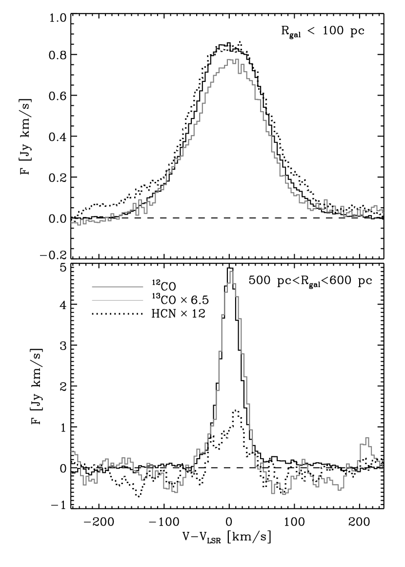
Figure 7.— Two examples of the spectra derived from the averaging process used to measure line ratios. The top panels shows the emission averaged over $R_{gal}<100$ pc and the bottom panel shows the average for $500\mbox{ pc}<R_{gal}<600\mbox{ pc}$. Emission from ${}^{13}\mbox{CO}$ has been scaled up by a factor of 6.5 and emission from HCN has been scaled up by a factor of 12. The line ratios change significantly over the face of the galaxy.

Figure 8.— Line ratios between molecular gas tracers as a function of galactocentric radius. Over most of the disk, the CO to ${}^{13}\mbox{CO}$ ratio has a values typical of the Milky Way disk ($\sim 6$) but shows a significant increase at small and large values of $R_{gal}$. For $R_{gal}>800$ pc, there are significant radial motions which may introduce systematic errors into the measurement technique. These increases may indicate significant amounts of diffuse molecular gas. The HCN/CO ratio is larger than seen in the GMCs in the Solar neighborhood, implying the average volume density of molecular gas is higher in M64 than it is in the Milky Way.

The value of $R_{13}$ changes significantly over the face of the galaxy with most of the molecular disk having a value of $R_{13}\sim 6$ comparable to the disk of the Milky Way. The nuclear region ($R_{gal}<200$ pc) and beyond $R_{gal}=800$ pc show an increased value of $R_{13}$. The material at small galactocentric radius may be affected by the presence of low-luminosity AGN and a nuclear starburst (Ho et al., 1997) which results in an increase in the kinetic temperature of the molecular gas. Such an increase in the temperature is thought to produce an increased value of $R_{13}$ near the nuclei of many galaxies (Paglione et al., 2001) and is consistent with the enhanced CO$(J=2\to 1)$/CO$(J=1\to 0)$ ratio observed at $R_{gal}\lesssim 100$ pc in the NUGA study. At large radii, the material may be disturbed by infalling material from the counter-rotating atomic disk beyond $R_{gal}=1000$ pc because the increase in $R_{13}$ is seen in gas where radial motions are observed (§3.1). The change in $R_{13}$ is probably because the fraction of gas in a diffuse, translucent phase is higher in this region than in the remainder of the galaxy. In both of these regions, the standard CO-to-H₂ conversion factor is suspect, since it is derived from gas where most of the molecular emission arises from cold, bound, opaque GMCs.

Near $R_{gal}\sim 0$, the ratio $W_{\mathrm{HCN}}/W_{\mathrm{CO}}$ is comparable to that seen in the nucleus of the Milky Way (Helfer & Blitz, 1997a) On average, the value of $W_{\mathrm{HCN}}/W_{\mathrm{CO}}$ over the entire galaxy is comparable to the value seen in the high column density regions of GMCs in the Solar neighborhood or the inner disk of the Milky Way. The relatively high values of this line ratio imply that a substantially larger fraction of the molecular gas is found in high density regions than is typical for the Solar neighborhood where $W_{\mathrm{HCN}}/W_{\mathrm{CO}}\lesssim 0.01$ (Helfer & Blitz, 1997a).

3.3. Fourier Analysis of the CO and ${}^{13}\mbox{CO}$ Line Ratios

The integrated intensity images of the CO and ${}^{13}\mbox{CO}$ emission look qualitatively different; the ${}^{13}\mbox{CO}$ emission looks significantly “clumpier.” Since the ${}^{13}\mbox{CO}$ emission should be a more faithful tracer of molecular column density than CO emission, the clumps seen in Figure 3 suggest that there are clouds present in the data. However, the ${}^{13}\mbox{CO}$ map also has lower dynamic range and the effects of masking may produce the difference in structure. In order to determine whether the ${}^{13}\mbox{CO}$ map is actually clumpier, we measured the variation in line ratio as a function of spatial scale using Fourier techniques. Since bound clouds have a fixed spatial scale ($\ell\sim 100$ pc in the Milky Way), emission arising from them should have most of its power around this scale. In contrast, emission from diffuse clouds is not limited to a fixed scale and should contribute at all spatial scales. Since the line ratio $R_{13}$ is different in diffuse vs. self-gravitating clouds, the ratio of power in the CO map to that of the ${}^{13}\mbox{CO}$ map should vary as a function of spatial scale.

We generated an integrated intensity map of the galaxy by shifting the emission in the spectra to a common velocity in order to eliminate the effects of galactic rotation. We integrated over a window 106.25 km s^-1 wide (25 channels) centered on the emission line. This generated integrated intensity maps with improved signal-to-noise without introducing any erroneous spatial filtering from masking the data. The resulting maps contained $>80\%$ of the emission found in the original maps with the missing emission in the nuclear region where the linewidth exceeds the width of the window. Next, we Fourier transformed the integrated intensity maps and averaged the power in elliptical annuli so that each annulus represents a range of scales in the deprojected image. We then subtracted the noise power from the data using the transform of noise images generated from emission-free regions of the data cube. The resulting power as a function of scale should represent only the power from line emission. In Figure 9 we plot the results of the analysis, scaling the ${}^{13}\mbox{CO}$ image up by the ratio of the fluxes at small scales (4.1) to facilitate comparison. The power spectra have the same shape at large scales ($\ell>200$ pc) and small scales ($75<\ell<200$ pc) but they have different ratios of powers in these two regimes: $6.5\pm 0.3$ for $\ell>200$ pc and $4.1\pm 0.1$ for $70<\ell<200$ pc. The value of $R_{13}$ at small scales is comparable to that seen in Galactic GMCs, and emission on these scales is from structures that may be the analogues of Galactic GMCs. Compared to the CO map, the ${}^{13}\mbox{CO}$ map has less emission at large scales where only diffuse gas should contribute. Hence, ${}^{13}\mbox{CO}$ emission from clouds will be less confused by the presence of diffuse gas compared to CO emission.

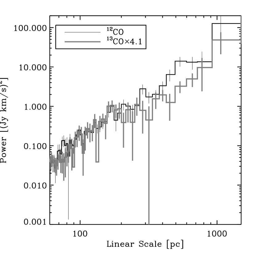
Figure 9.— Power spectrum of CO and ${}^{13}\mbox{CO}$ images as a function of spatial scale. The figure compares the power spectrum of the original CO data and the ${}^{13}\mbox{CO}$ image after being scaled by ratio of the fluxes at small spatial scales (4.1). The distribution of emission agrees well on the small scales but the line ratio at large spatial scale scales is larger (6.5). The difference in line ratios as a function of scale implies that the clumpy structure in Figure 3 is real and the line ratios are comparable to those seen in GMCs in the Milky Way.

The flux ratios derived in this analysis do not agree with the ratios calculated for the galaxy as a whole (Figure 8) for two reasons: (1) much of the emission with a large value of $R_{13}$ is located in the center of the galaxy where the velocity range is smaller than the linewidth so some high-$R_{13}$ emission is not included; and (2) incomplete subtraction of the noise power will skew the ratios to lower values. This is because the noise power, relative to the signal, is larger in the ${}^{13}\mbox{CO}$ emission. If there is incomplete subtraction of the noise, it will contribute more to the power in the ${}^{13}\mbox{CO}$ emission than to the CO emission.

The observed difference in flux ratios as a function of scale persists even when the dynamic range of the CO image is reduced to match that of the ${}^{13}\mbox{CO}$ image. We conclude that the different morphologies in Figures 2 and 3 represent a real difference in the structure of the emission from the galaxy and are not the result of the masking process. Furthermore, it appears that there is significant contribution to the molecular emission from a diffuse, translucent component of the molecular ISM. By analogy with molecular emission in the Milky Way, it is likely that it has a conversion factor $X_{2}<1$. Despite the lower signal-to-noise, the ${}^{13}\mbox{CO}$ map should be a better tracer of the molecular emission from bound clouds in M64. We return to the question of diffuse gas in §5.1.

4. Decomposition of the Molecular Emission

To answer the fundamental question of this study, namely ‘Are there GMCs in M64?’, we decompose the blended molecular emission into clouds and then compare the properties of these clouds with Local Group GMCs. For this purpose, we focus on the ${}^{13}\mbox{CO}$ emission since this tracer will be less contaminated by emission from diffuse molecular gas. There are three principal methods for isolating structures in blended molecular emission (1) partitioning of the cube by eye (e.g., Wilson & Scoville, 1990; Wright et al., 1993), (2) “cleaning” the data set by iteratively fitting and subtracting three dimensional Gaussians pioneered with the GAUSSCLUMPS algorithm by Stutzki & Güsten (1990) (3) partitioning of the emission by assigning it to the “closest” local maximum first developed in the CLUMPFIND algorithm by Williams et al. (1994). We adopt the latter approach for M64 since it does not require known functional forms for the ${}^{13}\mbox{CO}$ distribution of the clouds and it works directly with the emission present in the datacube. The original CLUMPFIND algorithm was implemented for the high signal-to-noise regime on single dish data. We have redeveloped the algorithm using the methods of Brunt et al. (2003) to make the method more robust in the presence of noise. In addition, we have modified the distance metric in the algorithm to be applicable to interferometer data which is oversampled in the spatial dimension. A detailed discussion of the algorithm appears in Appendix A, including benchmarking information for the choice of parameters. The algorithm can be applied to noisy, interferometric data with minimal variation in the properties of the derived clouds as a result of small changes in the free parameters of the algorithm.

Despite the modification of the algorithm to minimize the effects of of noise, decomposition of the ${}^{13}\mbox{CO}$ masked data used in Figure 3 was hampered by including low significance emission and noise. To improve the sensitivity of the datasets, we smoothed all three datacubes to a channel width of 8.5 km s^-1. We regenerated a mask for the CO data using the same method described in §3, namely we required $I>2\sigma_{rms}$ in a pixel that is connected to $I>4\sigma_{rms}$ detections in two adjacent channels. However, for the ${}^{13}\mbox{CO}$ and HCN data, we required $I>2\sigma_{rms}$ in two adjacent channels where there was detectable CO emission. The threshold was chosen so that $<1$ false detection would be included in the ${}^{13}\mbox{CO}$ and HCN masks. While this method discriminates against low significance emission, it does a far better job of selecting only real emission in the weaker tracers of molecular gas.

We applied the decomposition algorithm to the molecular emission in all three tracers. We also applied the algorithm to the CO data at the full velocity resolution because of the high signal-to-noise of the original CO data. In Figure 10, we display the masked, integrated intensity images for ${}^{13}\mbox{CO}$ and HCN, including the locations of the clouds into which the emission is decomposed. The algorithm isolates 87 clouds in the ${}^{13}\mbox{CO}$ emission and 42 clouds in the HCN. Only a fraction (25 and 9, respectively) of these clouds are resolved in both position and velocity space and these clouds are indicated with stars. The decomposition of the CO data at full velocity resolution yields 44 clouds. The algorithm identifies several clouds that appear in all three tracers with similar properties.

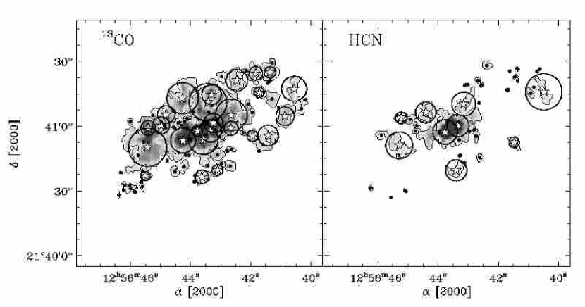
Figure 10.— The results of the decomposition algorithm applied to the ${}^{13}\mbox{CO}$ and HCN data sets. The locations of the clouds are overlaid on a grayscale integrated intensity maps of the galaxy. Locations of the clouds are indicated by stars (for clouds that are resolved in both position and velocity) and dots (unresolved in either position or velocity). The algorithm identifies 87 clouds in the ${}^{13}\mbox{CO}$ data, of which 25 are resolved, and 42 clouds in the HCN data, of which 9 are resolved. The effective radii ($R_{e}$, see Appendix B) of resolved clouds are indicated by the circle drawn around them. Several of the ${}^{13}\mbox{CO}$ clouds are also seen in the HCN emission with similar derived properties.

4.1. Cloud Properties

We measure the macroscopic properties of these clouds using intensity-weighted moments of the emission distribution, following the methods of Solomon et al. (1987) and Rosolowsky et al. (2003) to facilitate comparison with Local Group GMCs. Using these methods, we determine the mean position and line-of-sight velocity of each cloud. In addition, we measure three macroscopic properties for the clouds: the velocity FWHM ($\Delta V$), luminosity ($L$) and deconvolved effective radius ($R_{e}$). We have corrected the derived values for these properties to account for the fact that the data are clipped at $T_{clip}=2\sigma_{rms}$; and therefore, the properties are not measured over the same dynamic range as for Local Group clouds. To facilitate comparison with other data sets, we adopt the Gaussian correction used in Bolatto et al. (2003) and Oka et al. (2001). The derivation of the macroscopic cloud properties is given in detail in Appendix B. Table 3 is a listing of the cloud properties for the ${}^{13}\mbox{CO}$ clouds.

Table 3Properties of the resolved ${}^{13}\mbox{CO}$ clouds

Number	Position	$V_{LSR}$	$R_{e}$	$\Delta V$	$L_{\mathrm{13CO}}$	$P$
	(${}^{\prime\prime},^{\prime\prime}$)	[km s-1]	[pc]	[km s-1]	[$10^{4}$ K km s-1 pc2]
1	(29,–7)	266.1	176	28	87.4	4.7
2	(10,–4)	292.8	115	48	79.7	5.1
3	(–4,13)	473.5	174	68	67.0	3.6
4	(–16,7)	569.3	146	26	56.6	4.1
5	(–6,4)	539.1	89	39	55.1	4.2
6	(–1,–4)	401.6	136	73	54.8	3.8
7	(–5,0)	491.8	104	46	53.4	3.6
8	(10,15)	399.0	144	38	42.0	4.0
9	(28,1)	298.0	68	21	31.8	4.5
10	(2,0)	345.1	50	35	23.4	3.5
11	(19,8)	349.8	81	23	21.5	3.2
12	(22,3)	318.7	78	19	16.3	3.4
13	(–45,7)	550.6	86	18	15.8	3.3
14	(–19,24)	506.4	99	25	13.4	2.2
15	(–37,27)	544.0	53	18	13.4	3.8
16	(–16,1)	541.8	64	28	12.9	3.1
17	(–36,–2)	519.6	95	16	10.7	1.8
18	(–50,20)	581.3	115	16	10.3	2.3
19	(–29,27)	520.6	64	16	9.6	3.5
20	(–5,17)	493.3	90	19	8.2	1.7
21	(–9,–18)	404.6	50	10	7.2	2.5
22	(–31,18)	546.5	48	20	7.0	2.2
23	(0,–21)	380.3	62	23	5.4	2.4
24	(–27,–2)	509.4	51	12	4.9	1.9
25	(30,–21)	264.1	43	16	4.2	1.7

4.2. Comparison with Milky Way GMCs

In the Local Group, the macroscopic properties of molecular clouds are related by power law relationships, first noted by Larson (1981). In particular, the study of Solomon et al. (1987) found

$$\left(\frac{\Delta V}{\mbox{km s}^{-1}}\right)=1.7\left(\frac{R_{e}}{\mbox{pc}}\right)^{0.5}\mbox{ and }$$

$$\left(\frac{L_{\mathrm{12CO}}}{\mbox{K km s${}^{-1}$ pc${}^{-2}$}}\right)=1.8\left(\frac{\Delta V}{\mbox{km s}^{-1}}\right)^{5}.$$

We use these values for comparison with the results of this study since we have attempted to replicate their measurement methods and systematic effects. To compare the derived ${}^{13}\mbox{CO}$ luminosities to the luminosities of S87, which are measured in ¹²CO, we scale their relationship down by a factor of $R_{13}=6.7$, the global CO/${}^{13}\mbox{CO}$ line ratio, in the inner disk of the Milky Way (Polk et al., 1988). In Figure 11, we plot the relationships between these macroscopic properties for the clouds in M64. We have excluded clouds with linewidths larger than $\Delta V>60\mbox{ km s}^{-1}$. These clouds contain multiple peaks and appear to be the blend of two smaller clouds. These clouds are found near the center of the galaxy where the large velocity gradient makes decomposition of the emission difficult.

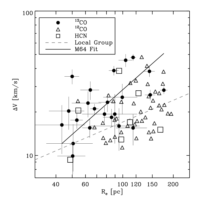
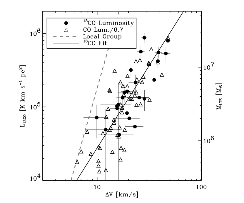
Figure 11.— Plot of the linewidth–size and luminosity–linewidth relationship for clouds in M64. The left-hand panel plots the relationship between cloud sizes and linewidths from the analysis of all three tracers. The right-hand panel plots the luminosity as a function of linewidth for the CO and ${}^{13}\mbox{CO}$ clouds. The luminosities of the CO clouds have been scaled down by 6.7 to compare them with the ${}^{13}\mbox{CO}$ clouds. The derived properties of the clouds are different from the corresponding Local Group trends plotted as dashed, gray lines. The M64 clouds appear to have smaller sizes or larger linewidths (or both) than clouds in the Local Group. For reference, the right-hand axis of the luminosity-linewidth plot indicates the luminous masses of the clouds assuming $X_{2}=1$ and $R_{13}=6.7$.

Several features are immediately apparent from Figure 11. First, the properties of the clouds are significantly different from the relationships derived by S87. Second, the clouds have large luminosities compared to the Local Group clouds. In S87, very few clouds are massive enough to have a ${}^{13}\mbox{CO}$ luminosity larger than $10^{5}\mbox{ K km s${}^{-1}$ pc${}^{2}$}$. For reference, the mass implied by the CO luminosity has also been plotted in Figure 11 assuming $R_{13}=6.7$ and $X_{2}=1$, which gives a ${}^{13}\mbox{CO}$-to-H₂ conversion factor equivalent to that derived using dust extinction by Lada et al. (1994). To compare the Milky Way and M64 clouds in a more quantitative fashion, we fit linear trends between $\log(R_{e})$, $\log(\Delta V)$ and $\log(L_{\mathrm{13CO}})$ for the ${}^{13}\mbox{CO}$ clouds using the method of Akritas & Bershady (1996), which is appropriate for a population with intrinsic scatter and measurements with errors in both parameters. We find that

$$\log\left(\Delta V\right) = (-0.6\pm 0.4)+(1.0\pm 0.3)\log\left(R_{e}\right)\mbox{ and }$$

$$\log\left(L_{\mathrm{13CO}}\right) = (2.2\pm 0.6)+(2.2\pm 0.4)\log\left(\Delta V\right).$$

The index for the linewidth–size is marginally different from the value for the Local Group ($1.0\pm 0.3$ vs. 0.5), and the luminosity-linewidth is significantly different from the Local Group trend ($2.2\pm 0.4$ vs. 5.0). These fits indicate that the clouds identified in the M64 data are not like molecular clouds seen in the disk of the Milky Way. However, the luminosity of these clouds implies that most of the clouds are significantly more massive than any clouds analyzed in the S87 study, and indeed Williams & McKee (1997) argue that no clouds more massive than $M>6\times 10^{6}~{}M_{\odot}$ will be found in the Milky Way disk. Thus, we are comparing the properties of these clouds with an extrapolation of Local Group clouds to high mass. It is noteworthy, however, that the low luminosity clouds in M64 have comparable luminosities, sizes and linewidths to the most massive clouds in the Milky Way. Thus, the M64 clouds may indicate a change in the scalings among GMC properties that occurs at high mass (or high average surface density). We cannot determine whether the apparent differences with respect to the S87 trends are an environmental effect or are intrinsic to high mass molecular clouds.

While the analysis has focused on the ${}^{13}\mbox{CO}$ clouds, Figure 11 shows that the clouds generated for other tracers have similar behaviors. Scaling the luminosity of the CO clouds down by 6.7 to place them on a similar scale as the ${}^{13}\mbox{CO}$ clouds produces a luminosity–linewidth relationship statistically indistinguishable from the relationship for the ${}^{13}\mbox{CO}$ clouds. In contrast, the sizes of the CO clouds appear significantly larger than the ${}^{13}\mbox{CO}$ clouds. A two-sided KS test indicates that the distributions of the CO and ${}^{13}\mbox{CO}$ cloud radii are significantly different ($P_{KS}>0.9993$), while the distributions of the linewidths are indistinguishable. We suspect that the larger CO radius results from the algorithm including the diffuse CO emission that surrounds the clouds in the definition of the CO clouds. To confirm this, we re-cataloged the CO emission clipping the map at $5\sigma_{rms}$, producing roughly the same dynamic range as the ${}^{13}\mbox{CO}$ map. The high clipping level eliminates the low surface brightness, diffuse CO emission. Our inclusion of a Gaussian extrapolation to a common clipping level facilitates direct comparison between the resulting catalogs. The clipped catalog contained 33 clouds; these clouds have sizes comparable to the ${}^{13}\mbox{CO}$ clouds, and a two-sided KS test found the distributions of both the sizes and the linewidths to be indistinguishable between the two tracers. The presence of diffuse emission can thus significantly affect the sizes of clouds traced by CO emission alone.

A major concern with the decomposition is whether the structures that the algorithm isolates really do represent discrete physical entities or whether the “clouds” are really blends of several small clouds that cannot be decomposed with the resolution of these observations. We suggest that this is not the case and that we are cataloging physical objects for several reasons. First, we tested the hypothesis that the clouds are blends of several GMCs like those found in the Milky Way by analyzing simulated data sets. For each data set, we constructed a population of 50 molecular clouds with a total mass of $2\times 10^{7}~{}M_{\odot}$ and individual masses drawn randomly from a mass distribution with $dN/dM\propto M^{-1.6}$. For each cloud in the simulation, we calculated the radius and linewidth that would be expected based on the study of S87. We randomly distributed these clouds in a data cube so that they would appear as a cloud with $R_{e}=$150 pc and $\Delta V=40$ km s^-1, which is appropriate for a typical massive cloud in our data set (Figure 11). We then convolved the simulated cube to the resolution of the observations and added noise to produce a peak signal-to-noise ratio of 8. We processed each simulated cube with the same masking and decomposition algorithm used in the data analysis. The algorithm identifies substructure within the data cubes in 90% of the trials, leading us to conclude that the clouds are not likely to be blends of a GMC population like that seen in the disk of the Milky Way.

The second piece of evidence that the decomposition products represent real objects is that the linewidths of the observed clouds, while large, are still significantly smaller than would be expected if the emission were composed of several smaller clouds orbiting in the galactic potential. We estimate the linewidth due to shear as

$$\Delta V_{shear}^{2}=\frac{\sum_{i}I(x_{i},y_{i})\cdot(\bar{v}-v_{r})^{2}(x_{i},y_{i})}{\sum_{i}I(x_{i},y_{i})}+\Delta V^{2}(x_{0},y_{0}),$$

where $I(x_{i},y_{i})$ is the integrated intensity at each position in the cloud, $(\bar{v}-v_{r})(x_{i},y_{i})$ is difference between the mean velocity and the line-of-sight projection of the rotation velocity at each position in the cloud, and $\Delta V^{2}(x_{0},y_{0})$ is the linewidth of the emission distribution at the cloud center. The final term accounts for broadening due to beam-smearing and the intrinsic gas velocity dispersion. The measured linewidth for the clouds ($\Delta V$ in Table 3) is smaller than $\Delta V_{shear}$ by a factor of 2.3 on average and does not change significantly with radius, even in the outer galaxy where the shear decreases.

Estimates of the cloud masses using the virial theorem agree well with estimates using the ${}^{13}\mbox{CO}$ emission, giving a third piece of evidence that we are identifying clouds. In particular, if we adopt the virial mass estimate used by S87,

$$\left(\frac{M_{\mathrm{VT}}}{M_{\odot}}\right)=187\left(\frac{\Delta V}{\mbox{km s}^{-1}}\right)^{2}\left(\frac{R_{e}}{\mbox{pc}}\right),$$ (1)

we find good correspondence between the virial mass estimates and luminous mass estimates as indicated in Figure 12. A linear fit between the log of the two mass estimates gives

$$\log(M_{\mathrm{VT}})=(-1.5\pm 1.2)+(1.2\pm 0.2)\log(M_{\mathrm{CO}}),$$

consistent with a direct correspondence between the mass estimates over an order of magnitude. This good agreement again suggests that the clouds are discrete objects, since the application of the virial theorem to unbound groups of molecular clouds gives virial masses significantly in excess of the mass estimated from the CO luminosity (e.g., Rand & Kulkarni, 1990; Rand, 1995; Allen & Lequeux, 1993). We have also used four alternate methods to measure the virial parameters (Heisler et al., 1985) and find no significant differences between the various methods.

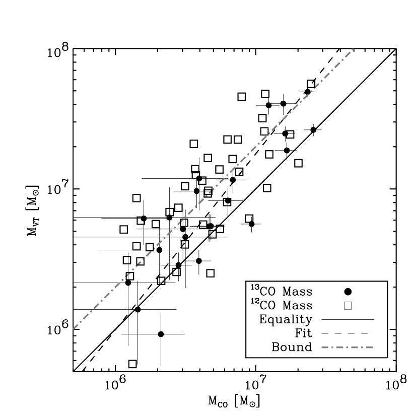
Figure 12.— Relationship between virial mass estimates and luminous mass estimates of the molecular gas for both ${}^{13}\mbox{CO}$ and CO clouds. The luminous mass estimates assume $X_{2}=1$ and $R_{13}=6.7$. The good correspondence between mass estimates for over an order of magnitude in mass implies that the clouds isolated by the algorithm are discrete physical entities, illustrated by a linear fit between the $\log(M_{\mathrm{VT}})$ and $\log(M_{\mathrm{CO}})$. The locus of marginally bound objects for $X_{2}=1$ and $R_{13}=6.7$ is shown as the dot-dashed gray line.

If the clouds represent self-gravitating objects, we can use the relationship between the luminous mass estimates and dynamical mass estimates to derive conversion factors for the tracers. Assuming the clouds are virialized, we perform a least-squares fit between $\log(M_{\mathrm{VT}})$ and $\log(L_{\mathrm{CO}})$, fixing the slope at unity to determine the scaling between these two tracers. Using these fits, we derive CO-to-H₂ conversion factors:

$$N(\mbox{H}_{2})=(1.8\pm 0.2)\times 10^{21}\mbox{ cm}^{-2}\cdot W_{\mathrm{13CO}}$$

$$N(\mbox{H}_{2})=(3.2\pm 0.2)\times 10^{20}\mbox{ cm}^{-2}\cdot W_{\mathrm{12CO}}\mbox{ or }X_{2}=(1.6\pm 0.1),$$

where the surface brightness $W$ is expressed in K km s^-1. If we assume the clouds are marginally bound instead of being virialized, we derive conversion factors that are a 2 times lower than these values. Given that the derived conversion factors bracket the measured values for both CO (Dame et al., 2001; Strong & Mattox, 1996) and ${}^{13}\mbox{CO}$ (Lada et al., 1994), it appears that dynamical estimates of the mass agree well with masses estimated from CO luminosity. Significant external pressure or the presence of magnetic fields will reduce the value of $M_{\mathrm{VT}}$, closing the small gap between the luminous ($X_{2}=1$, $R_{13}=6.7$) and virial mass estimates (McKee & Zweibel, 1992). In light of this, we adopt $X_{2}=1$ for the CO observations and the conversion factor of Lada et al. (1994) for the ${}^{13}\mbox{CO}$. Under the assumption of virialization, we also derive

$$\left(\frac{M}{M_{\odot}}\right)=(90\pm 10)\left(\frac{L_{\mathrm{HCN}}}{\mbox{K km s${}^{-1}$ pc${}^{-2}$}}\right),$$

implying HCN is brighter relative to CO in these clouds than is seen in Solar neighborhood GMCs (Helfer & Blitz, 1997a). However, HCN/CO ratio is similar to gas in the nuclear disk of the Milky Way where the mean density is higher.

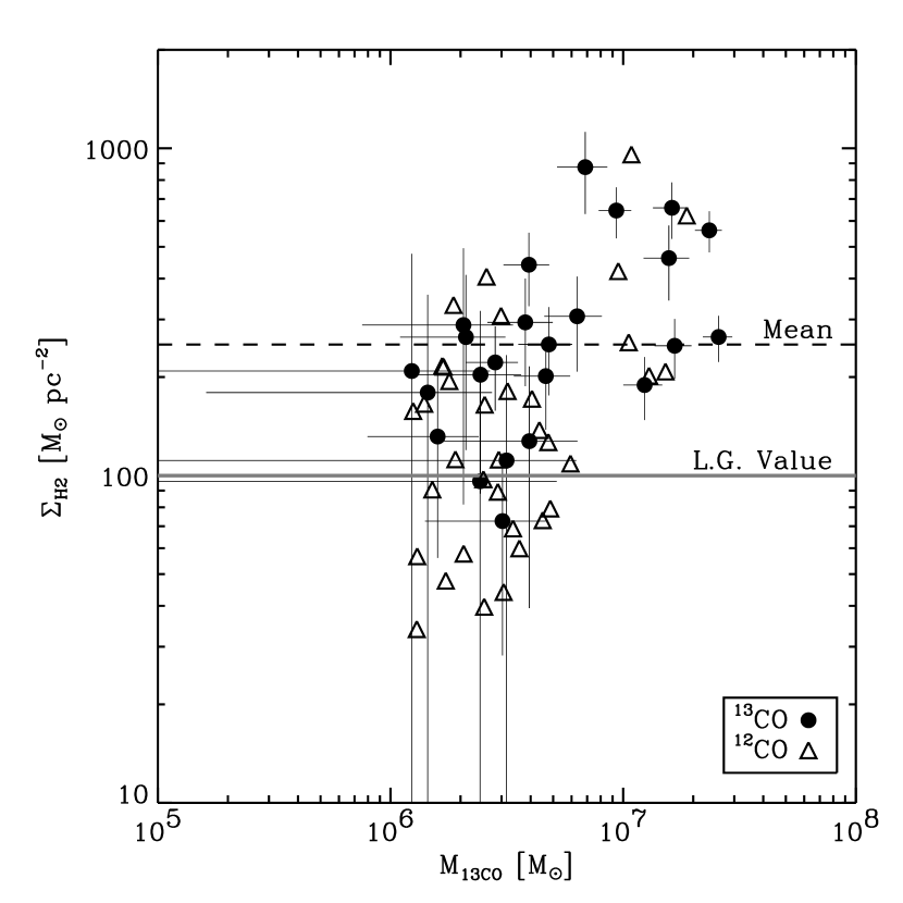
Figure 13.— The scaling of molecular surface density ($\Sigma_{\mathrm{H2}}$) with luminous mass $M_{\mathrm{13CO}}$. The molecular clouds in M64 have significantly higher surface densities than do clouds in the Milky Way. Moreover, the surface density is not constant with mass, as is necessary if the clouds are self-gravitating but follow a different size-linewidth relationship from clouds in the Local Group.

With mass measurements of the molecular clouds, we can convert these estimates to surface densities of the clouds. We plot the surface density of molecular gas in the clouds as a function of cloud mass in Figure 13. On average, the surface densities of the clouds are larger than are seen in the Milky Way with a mean value of $(250\pm 15)~{}M_{\odot}~{}\mbox{pc}^{-2}$, significantly higher than the value of $100~{}M_{\odot}~{}\mbox{pc}^{-2}$ seen in the Milky Way (Blitz, 1993) and M33 (Rosolowsky et al., 2003). In addition, the surface density is not constant with mass, which must be true if the clouds in the galaxies are self-gravitating but do not follow the same linewidth–size relationship as is observed in the Local Group. We find that

$$\Sigma_{\mathrm{H2}}\propto M^{0.7\pm 0.2}$$

meaning that high mass molecular clouds are systematically smaller and denser than would be expected from the extrapolation of trends seen in the Local Group. Moreover, an increased surface density of molecular gas also implies that the internal pressures of the molecular clouds are larger than are typical in the Local Group. We estimate the internal pressures of these clouds:

$$\frac{P_{int}}{k} \sim \langle\rho\rangle\sigma_{v}^{2}$$ (2)

$$= 212\mbox{ cm${}^{-3}$ K}\left(\frac{M}{M_{\odot}}\right)\left(\frac{R_{e}}{\mbox{pc}}\right)^{-3}\left(\frac{\Delta V}{\mbox{km s}^{-1}}\right)^{2}.$$

We find a mean internal pressure of $10^{6}$ K cm^-3, an order of magnitude larger than the value inferred for Milky Way GMCs (Blitz, 1993). However, an important quantity for comparison with the internal pressure is the mean external pressure exerted on the cloud by the ISM of M64. Blitz & Rosolowsky (2004) formulated an expression for the midplane hydrostatic pressure of the disks of galaxies:

$$\frac{P_{ext}}{k} = 272\mbox{ cm${}^{-3}$ K}\left(\frac{\Sigma_{gas}}{M_{\odot}\mbox{ pc}^{-2}}\right)\left(\frac{\Sigma_{*}}{M_{\odot}\mbox{ pc}^{-2}}\right)^{0.5}$$ (3)

$$\cdot\left(\frac{v_{g}}{\mbox{km s}^{-1}}\right)\left(\frac{h_{*}}{\mbox{pc}}\right)^{-0.5}$$

where $v_{g}$ is the 1-dimensional velocity dispersion of the gas, $h_{*}$ is the stellar scale height, and $\Sigma_{*}$ is the stellar surface density. We assume a gas velocity dispersion of $v_{g}=8$ km s^-1, corresponding to the linewidth of forbidden line emission in Rix et al. (1995). We derive an upper limit for the pressure by assuming and $h_{*}$ of 300 pc, typical of disk galaxies (Blitz & Rosolowsky, 2004). We measure $\Sigma_{*}$ derived from the 2MASS Large Galaxy Atlas image of M64 (Jarrett et al., 2003) assuming $M_{K}/L_{K}=0.5$ (Bell & de Jong, 2001). Finally, we take $\Sigma_{g}=\Sigma_{\mathrm{H2}}+\Sigma_{\mathrm{HI}}$. We calculate $\Sigma_{\mathrm{H2}}$ from the ${}^{13}\mbox{CO}$ surface density profile and use $\Sigma_{\mathrm{HI}}=10~{}M_{\odot}\mbox{ pc}^{-2}$ as measured in Braun et al. (1994). With these data, we compare the internal pressures of molecular clouds to the external pressure at the position of the cloud and find that the clouds are overpressured relative to the external medium by at least a factor of 2.

If we refine this estimate, the difference between $P_{int}$ and $P_{ext}$ grows larger. Of particular note, this estimate has included the contribution of the gas in self-gravitating molecular clouds in the contribution to the external pressure. These clouds likely do not contribute to the hydrostatic support of the ISM. Since this gas dominates the local column density, the actual external pressure is likely significantly smaller than the above estimate. If we use the estimate that 25% of the molecular gas is found in the diffuse component (§5.1) and assume that self-gravitating clouds do not contribute to the hydrostatic support of the ISM, then the clouds have internal pressures higher than the local ISM by a factor of 12, similar to the margin by which Solar neighborhood GMCs are overpressured with respect to the local ISM (Blitz, 1993). Recent star formation activity will decrease the mass-to-light ratio and therefore the mass estimate of the stellar disk, also reducing the external pressure. The central concentration of mass in GMCs tends to increase the internal pressures. Finally, the stellar scale height is likely larger than the 300 pc typical of galactic disks because of the presence of a significant bulge in the galaxy across the inner $\sim 300$ pc (Möllenhoff & Heidt, 2001).

Because the clouds are significantly overpressured with respect to the ambient medium, we take this as a final piece of evidence that the clouds are self-gravitating and that the luminosity traces molecular mass with conversion factors comparable to Milky Way values. Adding this to the agreement between the luminous and dynamical mass estimates and the small linewidths of the clouds, there is good evidence that molecular clouds identified by this method are gravitationally bound. The masses of many clouds are significantly larger than are seen in the disk of the Milky Way, where galactic tides set an upper limit to the mass of a GMC (Stark & Blitz, 1978). There is significant shear in the inner disk of M64 which may disrupt the clouds so we measured the tidal acceleration across each of the GMCs. We find that the clouds in Table 3 are marginally stable against tides using the methods of Stark & Blitz (1978). All clouds at $R_{gal}>400$ pc are very stable against tidal disruption. We conclude that these clouds are the analogues of the GMCs seen in the Milky Way, but have significantly different macroscopic properties.

4.3. Robustness of the Results

Several assumptions and choices have been incorporated in the conclusion that the molecular clouds observed in M64 are self-gravitating structures, analogous to high mass Giant Molecular Clouds. However, the principal results of our study do not change even if we relax these assumptions.

The largest influence on our cloud properties is the choice of the decomposition algorithm. The algorithm we developed has been designed to be robust against small variations in its parameters. Although we justify the choice of free parameters in Appendix A, we have re-cataloged the ${}^{13}\mbox{CO}$ emission while varying contouring levels and values of $T_{uniq}$ (the free parameters of the algorithm). We found all changes in the cloud properties were small and well within the uncertainties.

Because the clouds are comparable to the beam size, there is significant concern that the objects we catalog are the blends of several smaller clouds. We have argued in §4.2 that this is not the case, based on simulations, pressure arguments, dynamical mass estimates and cloud linewidths. Several of our results rely upon accurate decomposition of the emission. However, the most important of our results remain even if the clouds are blends of smaller structures. Namely, the surface (and volume) densities of the small clouds must be even higher than measured for the M64 clouds, implying they are even more over-pressured with respect to the ambient ISM; the estimate of the internal pressure (Equation 2) becomes a lower limit. Moreover, much of the following discussion (§5) is independent of how the clouds are decomposed. We also emphasize that the molecular structures cannot consist of Milky Way GMCs overlapping along the line of sight since Milky Way GMCs clouds are not dense enough to exist as discrete structures in the high-pressure molecular disk of M64.

The derived properties have been corrected for the finite signal-to-noise ratio in the dataset using a Gaussian extrapolation (see Appendix B). We have tested the validity of the Gaussian correction to the cloud properties by fitting three-dimensional Gaussians to the results of the decomposition. We find that the extrapolated values agree well with the fits. If we repeat the analyses of §4.2 without the corrections to their properties, we find (1) the indices of the linewidth–size and luminosity–linewidth relationships are still significantly different from the Local Group values, (2) the luminous and virial mass estimates still agree well, (3) the mean surface density of the clouds is $(450\pm 20)~{}M_{\odot}\mbox{ pc}^{-2}$, even higher than our adopted value and (4) the clouds are still significantly overpressured with respect to the ISM of M64.

Finally, the distance to M64 is somewhat uncertain with a recent estimate of $D=7.5$ Mpc (Tonry et al., 2001). Adopting a larger distance will change the values of the luminosity (as $D^{2}$) and the sizes (as $D$) but leave the linewidths unaffected. The indices of the scalings between the macroscopic properties will be invariant and remain different from the Local Group. The clouds will appear to have higher luminous masses relative to their virial masses ($M_{\mathrm{VT}}/M_{\mathrm{CO}}\propto D^{-1}$) and will still appear bound, though the derived conversion factors will be smaller. The surface densities of the molecular clouds do not vary with the adopted distance and will be significantly higher than Local Group values. While changing the adopted distance will alter the measured cloud properties, the main conclusions are robust: the most massive clouds in M64 appear to be self-gravitating structures with macroscopic properties significantly different from an extrapolation from Local Group GMCs.

5. Discussion

In this section, we relate the results of this study to molecular gas on galactic scales. We estimate the contribution of diffuse molecular gas to emission from M64 and examine the dust content and star-forming properties of the molecular clouds. Clarifying the properties of these high mass molecular clouds helps to link our understanding of star formation on small scales in the Milky Way to starbursts and ultraluminous infrared galaxies (ULIRGs).

5.1. The Fraction of Diffuse Gas in M64

Given the large CO to ${}^{13}\mbox{CO}$ line ratio ($R_{13}$) observed in some portions of M64, we suspect that a significant contribution of the emission arises from diffuse, translucent molecular gas. The resolved GMCs in Table 3 comprise $\sim$50% of the ${}^{13}\mbox{CO}$ emission from the galaxy. We cannot distinguish how much of the remaining emission arises from GMCs below our completeness limit or whether the emission arises from diffuse molecular gas.

Since emission from diffuse gas has a substantially different value of $R_{13}$ from that found in the GMCs, we can use our observations to establish the ratio of CO emission coming from diffuse gas vs. bound objects ($F\equiv W_{diff}/W_{GMC}$):

$$F=\frac{R_{diff}}{R_{GMC}}\frac{R_{avg}-R_{GMC}}{R_{diff}-R_{avg}}$$

where $R_{diff}$ is the line ratio in diffuse gas, $R_{GMC}$ is the line ratio in GMCs and $R_{avg}$ is the average of the line ratio over a given region (Polk et al., 1988; Wilson & Walker, 1994). Within the 25 clouds identified in the ${}^{13}\mbox{CO}$ emission, the line ratio $R_{13}=3.7$, which is typical of the peaks of emission from GMCs in our own galaxy (Polk et al., 1988). This suggests that the physical conditions averaged over these GMCs are comparable to the highest column density regions of GMCs in our own Galaxy. We assume that $R_{diff}=10\to 20$, which is appropriate for high-latitude clouds (Blitz et al., 1984; Magnani et al., 1985) and small clouds in the ISM (Knapp & Bowers, 1988). Then we can use the data in Figure 8 to estimate the fraction of diffuse emission in the different regions of the galaxy. From 200 pc $<R_{gal}<$ 800 pc, $R_{avg}\sim 6$ which implies, under these assumptions, that 40$\to$50% of the CO emission comes from GMCs and the balance comes from translucent molecular gas, comparable to the fraction seen in the Milky Way. A significant fraction (20%) of the CO emission comes from the inner 200 pc of the galaxy, around the AGN. Here, $R_{13}=8$ which implies that between 65% and 85% of the CO emission from the nucleus arises from diffuse molecular material which is equal to the fraction over the entire galaxy. In contrast, between 25% and 60% of the ${}^{13}\mbox{CO}$ emission comes from diffuse gas. Assuming the ${}^{13}\mbox{CO}$ emission linearly traces the molecular mass of the galaxy, we assume $R_{diff}=20$ and estimate that 25% of the molecular mass resides in diffuse structures and the remainder is in bound clouds.

The results of the Fourier analysis of the emission suggest a similar trend. In the ${}^{13}\mbox{CO}$ emission, the power on small ($\ell<200$ pc) scales comprises 20% of the total power, but for CO, this decreases to 10%. The Fourier analysis does not completely separate diffuse from bound emission since the diffuse component of the molecular ISM contributes power on small scales as well.

Line ratios indicate that a substantial portion of the molecular emission arises from diffuse gas, where the standard CO-to-H₂ conversion may be suspect. The ${}^{13}\mbox{CO}$-to-H₂ conversion factor is more appropriate for estimating the mass of the galaxy. Using $X_{2}=1$, we find that $M_{\mathrm{CO}}=(3.2\pm 0.4)\times 10^{8}~{}M_{\odot}$. Using the ${}^{13}\mbox{CO}$-to-H₂ conversion factor of Lada et al. (1994), we find $M_{\mathrm{13CO}}=(2.7\pm 0.1)\times 10^{8}~{}M_{\odot}$, roughly 30% of the Milky Way value (Dame, 1993). The two mass estimates for the molecular gas agree within the errors in the flux measurements, and the mass measurement of the gas appears robust. Using ${}^{13}\mbox{CO}$ emission to measure molecular mass will likely provide a more robust measurement of molecular mass in star-forming molecular clouds rather than the diffuse gas which is presumably inert with respect to star-formation.

5.2. Dust and Extinction in M64

Both CO isotopomers confirm a large mass of molecular gas in the inner kiloparsec of M64; and with the implied large column density of molecular material, there should be accompanying dust. Bendo et al. (2003) use ISO and SCUBA data to measure the long wavelength ($\lambda>100\mu\mbox{m}$) infrared and submillimeter emission from M64 and find an emission distribution consistent with two dust components at $T_{kin}=14$ K and 28 K respectively. The total dust mass implied by their observations is $2.7\times 10^{6}~{}M_{\odot}$ which implies a gas-to-dust ratio of $\sim 100$ by mass, very close to Galactic (Bohlin et al., 1978). If the molecular gas and the corresponding dust were distributed uniformly, the extinction through the disk should be $\sim A_{V}=7$. Stellar extinction measurements imply $A_{V}\sim 1.5$ (NUGA, Witt et al., 1994) implying that the dust (and gas) must have a filling fraction smaller than unity. The interferometer data show $\langle T_{A,max}\rangle=1.7$ K for CO but it is unlikely that the gas is significantly colder than $T_{kin}=10$ K or warmer than $T_{dust}=14~{}$K. If the difference is because of beam dilution, we estimate that the typical covering fraction of the gas in GMCs is $15\%\lesssim f\lesssim 45\%$.

5.3. Star Formation in M64

Large surface densities of molecular gas are linked to high star formation rates (Kennicutt, 1998; Wong & Blitz, 2002). In this section, we synthesize the results of the observations in several wavebands to determine if the star forming properties of the molecular gas in M64 are peculiar.

Using the FIR fluxes from the IRAS Bright Galaxy Sample (Soifer et al., 1989), and the scalings of Helou et al. (1988), we derive an FIR flux of $1.9\times 10^{-9}$ erg cm^-2 Hz^-1 from $S_{60}=30.2$ Jy and $S_{100}=78.7$ Jy. Scaling this with the relationship of Kennicutt (1998) yields a total SFR of 0.17 $M_{\odot}$ yr^-1 for $R_{gal}<1$ kpc or 0.05 $M_{\odot}$ yr^-1 kpc^-2, nearly an order of magnitude larger than in the Solar neighborhood (Miller & Scalo, 1979).

We synthesized a radio continuum spectral energy distribution from several studies in the literature (Condon et al., 1998; Turner & Ho, 1994; Israel & van der Hulst, 1983; Fanti et al., 1973) and derive

$$S(\nu)=(0.130\pm 0.005)\mathrm{\ Jy\ }\left(\frac{\nu}{1.4\mbox{ GHz}}\right)^{-0.61\pm 0.03}.$$

The radio continuum emission is confined to the molecular gas disk (Condon et al., 1998; Turner & Ho, 1994) and is well within the primary beam in all the interferometric studies. The resulting SFR is $0.15\pm 0.04~{}M_{\odot}$ yr^-1 using the formula of Condon (1992). Comparing this to the study of Murgia et al. (2002) indicates that M64 is quite similar to other galaxies with similar surface densities of molecular gas.

H$\alpha$ is one of the most commonly used star formation tracers in the galaxy, though using it requires correcting for extinction, which can be large. B94 use a wide field image and estimate the H$\alpha$ flux as $4.8\times 10^{-12}\exp(\langle\tau_{\mathrm{H}\alpha}\rangle)$ erg s^-1 cm^-2, where $\langle\tau_{\mathrm{H}\alpha}\rangle$ is the typical optical depth for H$\alpha$ emission, taken by Braun et al. (1994) to be 1.3. The corresponding star formation rate is 0.28 $M_{\odot}$ yr^-1 with the scalings of Kennicutt (1998). The Pa$\alpha$ image presented in §2.2 has a total flux of $9.3\times 10^{-13}\exp(\langle\tau_{\mathrm{Pa}\alpha}\rangle)$ erg s^-1 cm^-2. For a comparable degree of extinction as assumed in Braun et al. (1994), $\langle\tau_{\mathrm{Pa}\alpha}\rangle=0.23$ with the extinction law of Cardelli et al. (1989). This corresponds to a total star formation rate of 0.15 $M_{\odot}$ yr^-1 with the scaling of Kennicutt (1998). This is not unexpected since the image covers a smaller area than the H$\alpha$ image. The recombination line emission appears to accurately trace the star formation in the galaxy. In order for the line-of-sight extinction to the H II regions to be only $A_{V}=1.7$ while having the gas imply a mean extinction of $A_{V}=7$ again requires significant clumping of the molecular gas or else essentially all the H$\alpha$ emission would be extinguished by dust absorption.

The synthesis of observations suggest a star formation rate of $\sim$0.2 $M_{\odot}$ yr^-1, or 0.06 $M_{\odot}$ yr^-1 kpc^-2, over the molecular, star-forming disk. This agrees well with the high surface density regions of other molecule rich galaxies (Wong & Blitz, 2002; Murgia et al., 2002). Given the large density of molecular material present, the star formation activity is relatively quiescent, with a molecular gas depletion time of $\tau\gtrsim 1.4$ Gyr. Thus, the star formation efficiency of the molecular clouds is similar to that of the Milky Way (Mooney & Solomon, 1988).

5.4. The GMCs as Star Forming Structures

In §4.2, we argued that there are self-gravitating clouds of molecular gas in M64, though their properties are substantially different from the GMCs found in the disk of the Milky Way. These massive clouds also appear to be the star forming structures in M64. In Figure 14, we indicate the positions of molecular clouds from our catalog on the continuum subtracted HST image discussed in §2.2. Across the molecular disk, there is a strong correlation between GMCs and recombination emission from star formation. To quantify this, we convolved the H$\alpha$ image to the resolution of the ${}^{13}\mbox{CO}$ data and compared the brightness on a pixel by pixel basis. The correlation coefficient is $0.74\pm 0.02$ and rank correlation coefficient is $0.50\pm 0.03$. Performing a similar analysis with the Pa$\alpha$ image yields a correlation coefficient of $0.70\pm 0.02$ and $0.65\pm 0.02$. Star formation is clearly correlated with the gas in the Giant Molecular Clouds, but measuring the star formation rate within individual GMCs will require high resolution FIR observations. Unfortunately, the angular resolution of Spitzer observations will not be sufficient to correlate the FIR flux distribution with the location of GMCs.

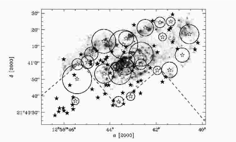
Figure 14.— – Locations of ${}^{13}\mbox{CO}$ molecular clouds overlaid on H$\alpha$ grayscale image. Resolved clouds are indicated with white stars and circles with of radius $R_{e}$ and unresolved clouds indicated with black stars. The border of the WFPC2 image is shown as a gray dashed line. Across the molecular disk, there is a correlation between GMCs and recombination emission, presumably from star formation.

Because the GMCs in M64 differ substantially from those of the Milky Way, they may have significantly different star formation efficiencies. However, the global star formation efficiency is not markedly enhanced. Studies throughout the Milky Way (Mooney & Solomon, 1988; Lis et al., 1991; Snell et al., 2002) show that that the star formation efficiency of clouds is constant with respect to cloud mass. On a large scale, it does not appear that the M64 clouds are peculiar in their star formation efficiency. This is not startling since even in ULIRGs there is evidence that the star formation efficiency is constant (Gao & Solomon, 2004). It is puzzling why such a large variation in the internal properties of GMCs results in a strikingly constant star formation efficiency.

5.5. Comparison to other GMCs in High Density Environments

There are several published studies searching for molecular clouds in high density environments. In particular, we compare the results of M64 to a CO study of the Antennae Galaxy (Arp 244) by Wilson et al. (2003) and CO observations of the Galactic center by Oka et al. (2001). Although the studies use different decomposition methods, it interesting to compare the results between the studies. We plot the mass–linewidth relationship for the studies under consideration in Figure 15. We choose to compare the mass–linewidth relationship since it avoids accurately measuring deconvolved radii of clouds across several studies. We include the study of S87 for comparison with these three studies in high density environments. The masses derived from CO luminosity have been rescaled to $X_{2}=1$.

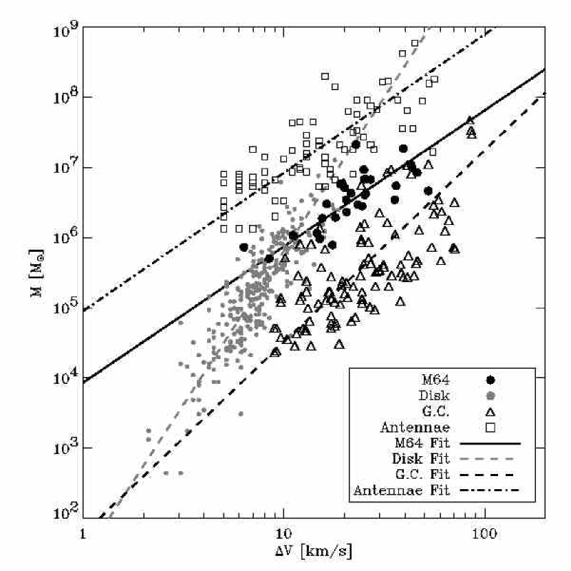
Figure 15.— The mass–linewidth relationship for four populations of GMCs. The GMCs from M64 are compared with those found in the Galactic center (Oka et al., 2001) the Antennae Galaxy (Wilson et al., 2003) and in the Galactic disk (Solomon et al., 1987, S87). All studies in high density systems have a similar mass–linewidth relationship $M\propto\Delta V^{2}$, which is dramatically different from the Milky Way relationship. The three high density cloud populations have significantly different offsets in the relationship.

Although all the studies use different methods for cloud decomposition, we directly compare their derived clouds to the M64 sample. Wilson et al. (2003) decomposed CO emission from the Antennae galaxies using the original CLUMPFIND algorithm, isolating massive molecular clouds. Performing a linear fit between $\log(\Delta V)$ and $\log(M_{\mathrm{CO}})$ for their data yields an index of $2.0\pm 0.1$, consistent with the M64 results and markedly different from the Milky Way values. The offset in luminosity is nearly an order of magnitude larger than the M64 data. Oka et al. (2001) decomposed the CO emission from the galactic center using the methods of S87. The index of their relationship is $(2.7\pm 0.2)$ and the offset is roughly an order of magnitude lower than the M64 clouds. In all three cases, the clouds follow a different mass-linewidth relationship than do Milky Way disk clouds.

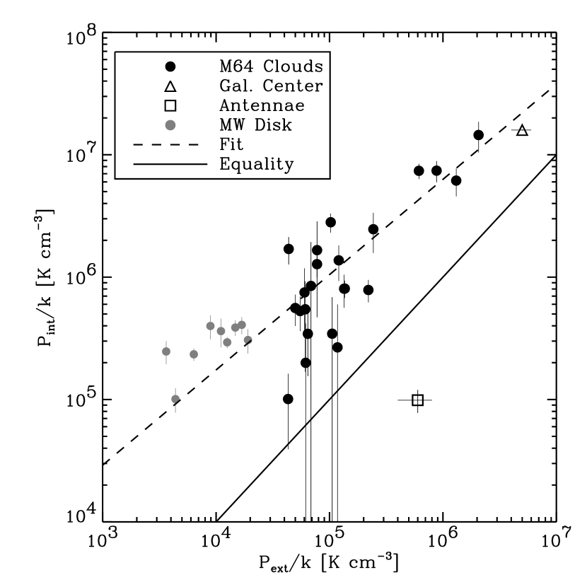
Figure 16.— A comparison of internal and external pressures for Giant Molecular Clouds in a variety of systems. Points represent pressure estimates in clouds for M64 (present work), Milky Way (S87), the Antennae galaxy (Wilson et al., 2003), and the Galactic center (Oka et al., 2001). Internal pressures are estimated from cloud properties. External pressures are quoted values from X-ray studies (Antennae, Galactic center) or estimated from the mass contributions of galactic components (Milky Way, M64). For most clouds, the internal pressure scales with the external pressure and is consistently above the derived value.

For 8 resolved clouds in the Antenna study, the virial masses agreed with the luminous mass estimates (for $X_{2}=1.5$) and the average surface density of the clouds is 100 $M_{\odot}\mbox{ pc}^{-2}$, comparable to the clouds of S87. On the opposite extreme, the mean surface density of the molecular clouds in the Galactic center is 500 $M_{\odot}\mbox{ pc}^{-2}$, higher than M64 clouds by a factor of 2. These differences are particularly interesting since they suggest that the high surface densities observed in M64 are not intrinsic to high mass GMCs but likely depend on environment. One environmental factor which may determine the properties of GMCs is the external hydrostatic pressure. GMCs cannot exist as discrete entities for much longer than a sound crossing-time unless they are self-gravitating and gravity is balanced by the internal pressure of the cloud. In environments that have high external pressures relative to the Milky Way, the internal pressures of clouds should be proportionally larger as well or else the pressure fluctuations in the diffuse ISM will destroy the clouds. To test the influence of environment on GMC properties, we plot the internal pressure of GMCs as a function of the external hydrostatic pressure for several galaxies (Figure 16). For M64 and the disk of the Milky Way, we estimate the pressure using methods described in §4. For M64, we assume that 1/4 of the molecular mass is diffuse and therefore contributes to the external pressure with $X_{2}=0.25$. We have included a point representing the mean surface density for GMCs estimated from the Galactic center data (Oka et al., 2001) at an external pressure of $P_{ext}/k=5\times 10^{6}\mbox{ K cm}^{-3}$ (Spergel & Blitz, 1992). We plot a point for the mean surface density of the sample of Wilson et al. (2003) using their estimate of the pressure, $P_{int}/k=6\times 10^{5}\mbox{ K cm}^{-3}$. Finally, we include the clouds of S87 and derive pressure values using the formula of Blitz & Rosolowsky (2004), the stellar density of Dehnen & Binney (1998) and the gas profile of Dame (1993). We have averaged the internal pressures of the clouds in bins of $\Delta P_{ext}/k=2\times 10^{3}\mbox{ K cm}^{-3}$ to highlight the significant scaling of internal pressure with external pressure within the S87 sample. This scaling is present using both luminous and dynamical mass estimates of the GMC in the Milky Way and implies a systematic variation of GMC column density with Galactic environment. There appears to be some offset between these populations, but this may be due to different methods for evaluating the pressure. The point representing the mean value for the Antennae galaxies is notably discrepant from the trend. This may be because the objects cataloged by Wilson et al. (2003) are physically distinct from those found in the other samples, perhaps because of the large spatial resolution of their study ($\theta_{beam}\sim 380$ pc). Omitting the point for the Antennae, we find a significant scaling with pressure: $P_{int}\propto P_{ext}^{0.75\pm 0.05}$. This scaling suggests that GMCs in molecule-rich, high-pressure environments are characteristically denser than those found in the Solar neighborhood. Since GMCs in M64 also show scaling of surface density with molecular mass, it is unclear as to whether the external pressure sets the surface densities of the cloud or whether high pressure environments form high mass clouds and the scaling with surface density is set by the cloud mass.

Table 4Summary of the GMC properties

	Milky Way	M64
Maximum Mass [$M_{\odot}$]	$6\times 10^{6}$	$2\times 10^{7}$
Size–Linewidth Scaling	$\Delta V\propto R_{e}^{0.5}$	$\Delta V\propto R_{e}^{1.0}$
Luminosity–Linewidth Scaling	$L\propto\Delta V^{5.0}$	$L\propto\Delta V^{2.2}$
Mass–Surface Density Scaling	$\Sigma_{\mathrm{H2}}\propto M^{0.0}$	$\Sigma_{\mathrm{H2}}\propto M^{0.7}$
$\langle\Sigma_{\mathrm{H2}}\rangle$ [$M_{\odot}~{}\mbox{pc}^{-2}$]	100	250
$\langle P_{int}\rangle$ [K cm-3]	$10^{5}$	$10^{6}$
SFR [$~{}M_{\odot}$ yr-1 kpc-2]	0.005	0.06
Mol. Gas Depletion Time [Gyr]	0.5	1.4

6. Summary and Conclusions

We have presented BIMA and FCRAO observations of the molecule rich galaxy M64 (NGC 4826) in the $(J=1\to 0)$ transition of three tracers: CO, ${}^{13}\mbox{CO}$ and HCN. The spatial resolution of the observations projects to 75 pc at the distance of M64, making it feasible to marginally resolve large molecular clouds in the galaxy. We decompose this emission into clouds that are high mass analogues of Giant Molecular Clouds in the Local Group. The properties of these clouds are significantly different from those seen locally and are summarized in Table 4. We report the following conclusions:

1. The line ratios $W_{\mathrm{CO}}/W_{\mathrm{13CO}}\equiv R_{13}$ and $W_{\mathrm{HCN}}/W_{\mathrm{CO}}$ vary over the face of the galaxy. The large values of $R_{13}$ seen in the nuclear regions of the galaxy ($R_{gal}<200$ pc) and beyond $R_{gal}=800$ pc imply substantial emission from diffuse molecular gas. Between these two regions, $R_{13}=6$, similar to the Milky Way disk. The ratio $W_{\mathrm{HCN}}/W_{\mathrm{CO}}$ declines monotonically from 0.09 in the middle of the galaxy to 0.012 at $R_{gal}=800$ pc.

2. A Fourier analysis of the emission distributions shows that the value of $R_{13}=4.1$ on small scales ($\ell<200$ pc) and $R_{13}=6.5$ on large scales. This implies that the clumpiness seen in the ${}^{13}\mbox{CO}$ image of the galaxy represents real cloud structures with values of $R_{13}$ comparable to Milky Way GMCs.

3. We decomposed the ${}^{13}\mbox{CO}$ emission into clouds and calculated their properties. We find several clouds with $M>10^{7}~{}M_{\odot}$ larger than any cloud seen in the disk of the Milky Way. The clouds show $L\propto\Delta V^{2.2\pm 0.4}$ which is a much smaller index than is seen for clouds in the Milky Way disk where $L\propto\Delta V^{5}$. Similarly, we find $\Delta V\propto R_{e}^{1.0\pm 0.3}$ compared to the Milky Way clouds where $\Delta V\propto R_{e}^{0.5}$. Despite these differences, virial estimates of their masses agree with those derived from the ${}^{13}\mbox{CO}$ emission for the Galactic ${}^{13}\mbox{CO}$to-H₂ conversion factor of Lada et al. (1994). The CO molecular clouds imply a COto-H₂ conversion factor of $(3.2\pm 0.2)\times 10^{20}\mbox{ cm}^{-2}\mbox{K~{}km~{}s}^{-1}$.

4. High mass GMCs in M64 are significantly smaller and denser than expected from extrapolating Local Group trends. The mean surface density of the M64 clouds is 250 $M_{\odot}\mbox{ pc}^{-2}$ and the surface density of the clouds varies with cloud mass: $\Sigma_{\mathrm{H2}}\propto M^{0.7\pm 0.2}$, compared to $\Sigma_{\mathrm{H2}}\propto$ const. in the Local Group. Clouds with masses comparable to those seen in the Milky Way also have comparable linewidths and radii, suggesting that the clouds may be similar for $M\sim 10^{6}~{}M_{\odot}$.

5. Diffuse gas (i.e. not bound in GMCs) contributes roughly 2/3 of the CO emission seen from the galaxy, but it only accounts for 1/4 the molecular mass in the galaxy. Nonetheless, empirically derived conversion factors for CO and ${}^{13}\mbox{CO}$ emission give a similar value of molecular mass for the entire galaxy: $2.7\times 10^{8}~{}M_{\odot}$ (for $D=4.1$ Mpc) for $X_{2}=1$

6. Recombination line emission, FIR and radiocontinuum measurements of the star formation rate M64 yield $\Sigma_{SFR}=0.06~{}M_{\odot}$ yr^-1 kpc^-2 or 0.2 $M_{\odot}$ yr^-1 for the central molecular disk. The molecular gas depletion time is $\sim$1.4 Gyr, comparable to similar galaxies.

7. The GMCs found in M64 are star forming structures, judging from their correlation with H$\alpha$ and Pa$\alpha$ emission in the galaxy. Despite the implied large values of their internal densities and pressures, the star formation efficiency is not dramatically enhanced. The GMCs in M64 share many qualities with GMCs found in the center of the Milky Way.

8. The GMCs in M64 share many properties with populations of clouds found in the inner Milky Way and the Antennae galaxy. GMCs in all three galaxies have a well-defined mass–linewidth relationship with an index $\sim 2$, markedly different from the clouds in the inner disk of the Milky Way. We the internal pressure of GMCs scales with the external pressure of the ISM: $P_{int}\propto P_{ext}^{0.75\pm 0.05}$.

Appendix A The Modified CLUMPFIND Algorithm

In this paper, we use a modified CLUMPFIND (Williams et al., 1994, WGB94) algorithm since we seek maximum flexibility in identifying the geometry of the molecular emission. The dataset we are analyzing in this paper is significantly different from that of WGB94, who used single dish data that were spatially Nyquist sampled. In contrast, the interferometer data has several pixels across a beam and is often at lower signal-to-noise than the data examined by WGB94. To optimize the CLUMPFIND method for our data, we adopt two significant changes. First, we determine which local maxima to include in the analysis before dividing the emission into clouds corresponding to those peaks. This allows a more careful analysis in the relatively low signal-to-noise domain. The other change we adopt is to change the path length metric so that path segments in velocity are a factor of $w_{v}\equiv\theta_{FWHM}/2\Delta x$ longer than path segments in velocity. $w_{v}$ is the number of spatial pixels per beam half-width, roughly 4 in these data. This change accounts for the oversampling in the spatial direction of our data. A graphic representation of the distance metric adopted in the datacube is shown in Figure 17.

Accurate selection of significant local maxima is the key to implementing our algorithm. In WGB94, significant local maxima are determined by contouring the data in units of $\Delta T/\sigma_{rms}=2$, descending through the contour levels, and marking any new, isolated island at a given contour level as a new maximum. However, a noise fluctuation can cause an artificial local maximum and a false clump and the choice $\Delta T/\sigma_{rms}=2$ is a compromise between discriminating against noise spikes (large contouring interval) and sensitivity to emission structure (small contour level). To optimize the algorithm, we separate these two criteria: adopting a small contouring level to follow the emission structure well while keeping track of the levels at which isolated regions merge in order to later determine whether certain “clouds” represent noise spikes. We adopt a similar method to (and heavily inspired by) the work of Brunt et al. (2003). In their method, two local maximum are considered distinct if the saddle point connecting them is at least $\Delta T_{uniq}/\sigma_{rms}$ below both maxima. Brunt et al. (2003) use $\Delta T_{uniq}/\sigma_{rms}=4$ but we find a value of 3.0 is appropriate for our data (see Figure 18). In our method, we contour the data in units of $0.5\sigma_{rms}$, and record isolated islands that appear in each contour level as well as the level at which pairs of maxima merge. If a maximum merges with another, higher maximum and the saddle point between the maxima is less than $\Delta T_{uniq}/\sigma_{rms}$, it is considered to be the same cloud and the smaller local maximum is removed from the analysis. This selects against noise spikes since they appear as isolated maxima in a single resolution element of the datacube whereas cloud structures appear in multiple elements. Once all connected local maxima are tested for the presence of noise, the remaining local maxima are used to partition the data set.

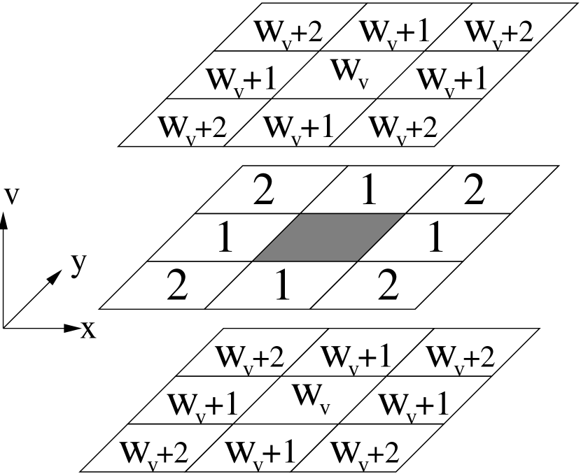
Figure 17.— Distances from the central shaded pixels to adjacent pixels in the data cube. The number $w_{v}$ accounts for the oversampling in the spatial direction by making different velocity planes correspondingly “farther” from the central pixel. Within a given plane, only the four pixels immediately adjacent to the central pixel are considered neighbors and, consequently, one distance unit away. This definition results in a “taxicab metric” in a given plane.

The data set is partitioned by stepping downward from the maximum value of $T_{A}$ in units of $0.5\sigma_{rms}$. Pixels added at each level are assigned to the local maximum that has the shortest path through the datacube connecting the pixel to that maximum. Paths are constrained to run through pixels which contain emission, and the length of a path between two pixels is defined as the minimum length over all possible paths that lie within the bounds of the emission. Steps in velocity are considered to be a factor of $w_{v}=\theta_{FWHM}/2\Delta x$ longer than steps in position space. If pixel is connected to two maxima by paths of equal length, then the pixel is assigned to the closest pixel using a Euclidean distance metric:

$$d(\mathbf{x}_{1},\mathbf{x}_{2})=\sqrt{(x_{1}-x_{2})^{2}+(y_{1}-y_{2})^{2}+w_{v}^{2}(v_{1}-v_{2})^{2}}.$$ (A1)

Here, $w_{v}$ is the same factor that accounts for oversampling in the spatial direction. If the pixels have equivalent path and Euclidean distances to two separate maxima, the pixel is assigned randomly to one.

To evaluate the optimal parameters in running the algorithm, we performed Monte Carlo simulations on controlled simulations. The simulated data consisted of two clouds with Gaussian profiles in position and velocity space. Interferometer noise was added to some trials to mimic the observation conditions. Ideally, the algorithm will consistently separate the blended Gaussians into (only) two clouds. By varying the signal-to-noise, Gaussian separation and algorithm parameters, we explored the limitations of the algorithm and the ideal parameters for decompositions. In Figure 18, we display the results of two such experiments. First, we fixed the cloud separation at $3\sigma_{x}$ and varied the peak signal-to-noise to determine the limitations imposed by noise on the decomposition. For $\Delta T_{uniq}/\sigma_{rms}=3$, we find that our modified CLUMPFIND algorithm consistently recovers two clouds while the original CLUMPFIND finds a significantly larger number owing to the presence of noise. The modified algorithm breaks down when the signal-to-noise ratio is less than 5. In the second panel of Figure 18, we compare the number of clouds resulting from the decomposition as a function of cloud separation and $\Delta T_{uniq}/\sigma_{rms}$. This experiment explores the ability of the algorithm to separate blended clouds and motivates our selection of $\Delta T_{uniq}/\sigma_{rms}=3$. We choose a signal-to-noise ratio of 8 for the trials. Selecting $\Delta T_{uniq}/\sigma_{rms}<3$ results in noise spikes causing a spurious decomposition of the clouds. Selecting $\Delta T_{uniq}/\sigma_{rms}>3$ does not significantly change the results of the decomposition. The algorithm successfully separates clouds with a separation between them of $\Delta x/\sigma_{x}\gtrsim 3$.

Figure 18.— Benchmarking results for the modified CLUMPFIND algorithm. In the left-hand panel we plot the number of clouds the algorithm that result from decomposing a trial data set as a function of signal to noise. The modified algorithm produces good results even down to a peak signal-to-noise value of 5. In contrast, the CLUMPFIND algorithm displays large sensitivity to noise in the low signal-to-noise regime. In the right-hand panel, we plot the number of clouds that result from decomposition as a function of cloud separation for $T_{peak}/\sigma_{rms}=8$. The trials are conducted using a range of values for the algorithm parameter $\Delta T_{uniq}/\sigma_{rms}$, which determines the algorithm’s sensitivity to noise. The trials show that $\Delta T_{uniq}/\sigma_{rms}=3$ is reproduces the model well while not requiring extremely high signal-to-noise in the data and that for this choice, the algorithm separates the two model clouds for $\Delta x/\sigma_{x}\gtrsim 3$.

We have also checked the influence on choice of contour levels and find that a contouring the data in levels smaller 0.5 $\sigma_{rms}$ does not change the outcome of the decomposition. We use 0.5$\sigma_{rms}$ in our analysis of the data. In addition, we also check the ratio of fluxes in the resulting clouds for trial clouds with unequal intensities; and we find that the algorithm partitions the clouds reasonably.

Appendix B Derivation of Cloud Properties

Using intensity-weighted moments, we have calculated the macroscopic properties of the clouds in M64. The position of the cloud is taken as the centroid position, weighted by the antenna temperature in each pixel $T_{i}$, e.g., $x_{0}=(\sum_{i}T_{i}x_{i})/(\sum_{i}T_{i})$. The linewidth and radius of the cloud are calculated by taking the second moment of the emission in velocity and position respectively:

$$\sigma_{r}^{2} = \frac{1}{\sum_{i}T_{i}}\sum_{i}T_{i}\left[\left(x-x_{0}\right)^{2}+\left(y-y_{0}\right)^{2}\right]$$ (B1)

$$\sigma_{v}^{2} = \frac{1}{\sum_{i}T_{i}}\sum_{i}T_{i}\left(v-v_{0}\right)^{2}$$ (B2)

To transform the moments into cloud radii and linewidths, we first corrected the derived moments for the effects of clipping, since the lowest contour level is at $T_{A}=2\sigma_{rms}$ rather than zero. As such, the derived moments underestimate the true $\sigma_{r}^{2}$ and $\sigma_{v}^{2}$ of the cloud. In order to compensate, we assumed the clouds have a Gaussian profile in position-position-velocity space. Since the clouds are only marginally resolved at best, the assumption of a Gaussian profile seems to be reasonable. We correct the moments by the ratio of the value of the moment extrapolated to a common reference value to the value of the moment for emission clipped at $T_{A}=2\sigma_{rms}$ (Oka et al., 2001; Bolatto et al., 2003). The correction factor depends solely upon the peak-to-edge ratio, $P\equiv T_{max}/T_{clip}$ where $T_{max}$ is the maximum antenna temperature in the emission region and $T_{clip}$ is the clipping level, equal to $2\sigma_{rms}$ for this study. In this case, the correction factor, $f(P)$, is

$$f(P) = \left[\frac{\int_{0}^{x_{ref}}x^{4}\exp(-x^{2}/2)}{\int_{0}^{x_{ref}}x^{2}\exp(-x^{2}/2)}\right]\cdot\left[\frac{\int_{0}^{x_{max}}x^{4}\exp(-x^{2}/2)}{\int_{0}^{x_{max}}x^{2}\exp(-x^{2}/2)}\right]^{-1}\mbox{ where }$$ (B3)

$$x_{max} = \sqrt{2\ln(P)}\mbox{ and }x_{ref}=2$$

The clouds in Solomon et al. (1987) typically have $P=8$ implying, for that sample, $x_{max}=\sqrt{2\ln(8)}=2.04$. To match the clipping levels used in that study, we choose the reference value for the extrapolation $x_{ref}=2$. For a typical cloud which has $P=3.5$, $f(P)=1.4$ resulting in a correction of 20% to the size and linewidth of the cloud.

The linewidth is calculated by scaling the corrected dispersion to a FWHM using the Gaussian linewidth correction: $\Delta V=\sigma_{v}\cdot\sqrt{f(P)8\ln(2)}$. The cloud radius is derived by correcting $\sigma_{r}$ for clipping and beam convolution and then applying the scaling from $\sigma_{r}$ used by Solomon et al. (1987) in their study of Milky Way clouds:

$$R_{e}=\frac{3.4}{\sqrt{2\pi}}\sqrt{f(P)\sigma_{r}^{2}-2\sigma_{beam}^{2}}.$$ (B4)

Our simple model to correct $R_{e}$ for beam convolution breaks down when $\sigma_{r}\sqrt{f(P)}<\sigma_{beam}$, and so we only consider a cloud resolved if $R_{e}>40\mbox{ pc}$. Similarly, we only consider a cloud to be resolved in the velocity direction if $\Delta V$ is larger than the channel width.

The luminosity of the cloud is also reduced by clipping the cloud at $2\sigma_{rms}$. To account for this clipping, we correct the integrated intensity value by a factor of

$$g(P)=\frac{\int_{0}^{x_{ref}}x^{2}\exp(-x^{2}/2)}{\int_{0}^{x_{max}}x^{2}\exp(-x^{2}/2)}$$ (B5)

For clouds with $P=3.5$, the correction factor $g(P)=1.4$ for $x_{ref}=2$. The dominant source of uncertainty comes from the extrapolation of cloud properties using the correction factors $f(P)$ and $g(P)$, though most of our conclusions are independent of applying this correction. In this paper, we have assigned the derived quantities an uncertainty equal to half the value of this correction.

References

- Aalto et al. (1995) Aalto, S., Booth, R. S., Black, J. H., & Johansson, L. E. B. 1995, A&A, 300, 369
- Akritas & Bershady (1996) Akritas, M. G. & Bershady, M. A. 1996, ApJ, 470, 706
- Allen & Lequeux (1993) Allen, R. J. & Lequeux, J. 1993, ApJ, 410, L15
- Böker et al. (1999) Böker, T., Calzetti, D., Sparks, W., Axon, D., Bergeron, L. E., Bushouse, H., Colina, L., Daou, D., Gilmore, D., Holfeltz, S., MacKenty, J., Mazzuca, L., Monroe, B., Najita, J., Noll, K., Nota, A., Ritchie, C., Schultz, A., Sosey, M., Storrs, A., & Suchkov, A. 1999, ApJS, 124, 95
- Begeman (1989) Begeman, K. G. 1989, A&A, 223, 47
- Bell & de Jong (2001) Bell, E. F. & de Jong, R. S. 2001, ApJ, 550, 212
- Bendo et al. (2003) Bendo, G. J., Joseph, R. D., Wells, M., Gallais, P., Haas, M., Heras, A. M., Klaas, U., Laureijs, R. J., Leech, K., Lemke, D., Metcalfe, L., Rowan-Robinson, M., Schulz, B., & Telesco, C. 2003, AJ, 125, 2361
- Blitz (1993) Blitz, L. 1993, in Protostars and Planets III, 125–161
- Blitz et al. (1984) Blitz, L., Magnani, L., & Mundy, L. 1984, ApJ, 282, L9
- Blitz & Rosolowsky (2004) Blitz, L. & Rosolowsky, E. 2004, ApJ, 612, L29
- Bohlin et al. (1978) Bohlin, R. C., Savage, B. D., & Drake, J. F. 1978, ApJ, 224, 132
- Bolatto et al. (2003) Bolatto, A. D., Leroy, A., Israel, F. P., & Jackson, J. M. 2003, ApJ, 595, 167
- Braun et al. (1994) Braun, R., Walterbos, R. A. M., Kennicutt, R. C., & Tacconi, L. J. 1994, ApJ, 420, 558 (B94)
- Brunt et al. (2003) Brunt, C. M., Kerton, C. R., & Pomerleau, C. 2003, ApJS, 144, 47
- Cardelli et al. (1989) Cardelli, J. A., Clayton, G. C., & Mathis, J. S. 1989, ApJ, 345, 245
- Casoli & Gerin (1993) Casoli, F. & Gerin, M. 1993, A&A, 279, L41
- Condon (1992) Condon, J. J. 1992, ARA&A, 30, 575
- Condon et al. (1998) Condon, J. J., Cotton, W. D., Greisen, E. W., Yin, Q. F., Perley, R. A., Taylor, G. B., & Broderick, J. J. 1998, AJ, 115, 1693
- Dame (1993) Dame, T. M. 1993, in AIP Conf. Proc. 278: Back to the Galaxy, 267–278
- Dame et al. (2001) Dame, T. M., Hartmann, D., & Thaddeus, P. 2001, ApJ, 547, 792
- de Vries et al. (1987) de Vries, H. W., Thaddeus, P., & Heithausen, A. 1987, ApJ, 319, 723
- Dehnen & Binney (1998) Dehnen, W. & Binney, J. 1998, MNRAS, 294, 429
- Engargiola et al. (2003) Engargiola, G., Plambeck, R. L., Rosolowsky, E., & Blitz, L. 2003, ApJS, 149, 343
- Fanti et al. (1973) Fanti, R., Gioia, I., Lari, C., Lequeux, J., & Lucas, R. 1973, A&A, 24, 69
- Gao & Solomon (2004) Gao, Y. & Solomon, P. M. 2004, ApJ, 606, 271
- García-Burillo et al. (2003) García-Burillo, S., Combes, F., Hunt, L. K., Boone, F., Baker, A. J., Tacconi, L. J., Eckart, A., Neri, R., Leon, S., Schinnerer, E., & Englmaier, P. 2003, A&A, 407, 485 (NUGA)
- Heisler et al. (1985) Heisler, J., Tremaine, S., & Bahcall, J. N. 1985, ApJ, 298, 8
- Helfer & Blitz (1997a) Helfer, T. T. & Blitz, L. 1997a, ApJ, 478, 233
- Helfer & Blitz (1997b) —. 1997b, ApJ, 478, 162
- Helfer et al. (2003) Helfer, T. T., Thornley, M. D., Regan, M. W., Wong, T., Sheth, K., Vogel, S. N., Blitz, L., & Bock, D. C.-J. 2003, ApJS, 145, 259
- Helou et al. (1988) Helou, G., Khan, I. R., Malek, L., & Boehmer, L. 1988, ApJS, 68, 151
- Ho et al. (1997) Ho, L. C., Filippenko, A. V., & Sargent, W. L. W. 1997, ApJS, 112, 315
- Israel & van der Hulst (1983) Israel, F. P. & van der Hulst, J. M. 1983, AJ, 88, 1736
- Jarrett et al. (2003) Jarrett, T. H., Chester, T., Cutri, R., Schneider, S. E., & Huchra, J. P. 2003, AJ, 125, 525
- Kennicutt (1998) Kennicutt, R. C. 1998, ApJ, 498, 541
- Knapp & Bowers (1988) Knapp, G. R. & Bowers, P. F. 1988, ApJ, 331, 974
- Lada et al. (1994) Lada, C. J., Lada, E. A., Clemens, D. P., & Bally, J. 1994, ApJ, 429, 694
- Larson (1981) Larson, R. B. 1981, MNRAS, 194, 809
- Lis et al. (1991) Lis, D. C., Carlstrom, J. E., & Keene, J. 1991, ApJ, 380, 429
- Möllenhoff & Heidt (2001) Möllenhoff, C. & Heidt, J. 2001, A&A, 368, 16
- Magnani et al. (1985) Magnani, L., Blitz, L., & Mundy, L. 1985, ApJ, 295, 402
- Magnani et al. (2003) Magnani, L., Chastain, R. J., Kim, H. C., Hartmann, D., Truong, A. T., & Thaddeus, P. 2003, ApJ, 586, 1111
- McKee & Zweibel (1992) McKee, C. F. & Zweibel, E. G. 1992, ApJ, 399, 551
- Meier (2002) Meier, D. S. 2002, Ph.D. Thesis (M02)
- Miller & Scalo (1979) Miller, G. E. & Scalo, J. M. 1979, ApJS, 41, 513
- Mizuno et al. (2001) Mizuno, N., Yamaguchi, R., Mizuno, A., Rubio, M., Abe, R., Saito, H., Onishi, T., Yonekura, Y., Yamaguchi, N., Ogawa, H., & Fukui, Y. 2001, PASJ, 53, 971
- Mooney & Solomon (1988) Mooney, T. J. & Solomon, P. M. 1988, ApJ, 334, L51
- Murgia et al. (2002) Murgia, M., Crapsi, A., Moscadelli, L., & Gregorini, L. 2002, A&A, 385, 412
- Oka et al. (2001) Oka, T., Hasegawa, T., Sato, F., Tsuboi, M., Miyazaki, A., & Sugimoto, M. 2001, ApJ, 562, 348
- Paglione et al. (2001) Paglione, T. A. D., Wall, W. F., Young, J. S., Heyer, M. H., Richard, M., Goldstein, M., Kaufman, Z., Nantais, J., & Perry, G. 2001, ApJS, 135, 183
- Polk et al. (1988) Polk, K. S., Knapp, G. R., Stark, A. A., & Wilson, R. W. 1988, ApJ, 332, 432
- Rand (1995) Rand, R. J. 1995, AJ, 109, 2444
- Rand & Kulkarni (1990) Rand, R. J. & Kulkarni, S. R. 1990, ApJ, 349, L43
- Regan et al. (2001) Regan, M. W., Thornley, M. D., Helfer, T. T., Sheth, K., Wong, T., Vogel, S. N., Blitz, L., & Bock, D. C.-J. 2001, ApJ, 561, 218
- Rix et al. (1995) Rix, H. R., Kennicutt, R. C., Braun, R., & Walterbos, R. A. M. 1995, ApJ, 438, 155
- Rosolowsky et al. (2003) Rosolowsky, E. W., Plambeck, R., Engargiola, G., & Blitz, L. 2003, ApJ, 599, 258
- Rubin (1994) Rubin, V. C. 1994, AJ, 107, 173
- Snell et al. (2002) Snell, R. L., Carpenter, J. M., & Heyer, M. H. 2002, ApJ, 578, 229
- Soifer et al. (1989) Soifer, B. T., Boehmer, L., Neugebauer, G., & Sanders, D. B. 1989, AJ, 98, 766
- Solomon et al. (1987) Solomon, P. M., Rivolo, A. R., Barrett, J., & Yahil, A. 1987, ApJ, 319, 730 (S87)
- Spergel & Blitz (1992) Spergel, D. N. & Blitz, L. 1992, Nature, 357, 665
- Stanimirovic et al. (1999) Stanimirovic, S., Staveley-Smith, L., Dickey, J. M., Sault, R. J., & Snowden, S. L. 1999, MNRAS, 302, 417
- Stark & Blitz (1978) Stark, A. A. & Blitz, L. 1978, ApJ, 225, L15
- Strong & Mattox (1996) Strong, A. W. & Mattox, J. R. 1996, A&A, 308, L21
- Stutzki & Güsten (1990) Stutzki, J. & Güsten, R. 1990, ApJ, 356, 513
- Teuben (1995) Teuben, P. 1995, in ASP Conf. Ser. 77: Astronomical Data Analysis Software and Systems IV, 398–+
- Tonry et al. (2001) Tonry, J. L., Dressler, A., Blakeslee, J. P., Ajhar, E. A., Fletcher, A. B., Luppino, G. A., Metzger, M. R., & Moore, C. B. 2001, ApJ, 546, 681
- Tully (1988) Tully, R. B. 1988, Nearby galaxies catalog (Cambridge and New York, Cambridge University Press, 1988, 221 p.)
- Turner & Ho (1994) Turner, J. L. & Ho, P. T. P. 1994, ApJ, 421, 122
- Welch et al. (1996) Welch, W. J., Thornton, D. D., Plambeck, R. L., Wright, M. C. H., Lugten, J., Urry, L., Fleming, M., Hoffman, W., Hudson, J., Lum, W. T., Forster, J. . R., Thatte, N., Zhang, X., Zivanovic, S., Snyder, L., Crutcher, R., Lo, K. Y., Wakker, B., Stupar, M., Sault, R., Miao, Y., Rao, R., Wan, K., Dickel, H. R., Blitz, L., Vogel, S. N., Mundy, L., Erickson, W., Teuben, P. J., Morgan, J., Helfer, T., Looney, L., de Gues, E., Grossman, A., Howe, J. E., Pound, M., & Regan, M. 1996, PASP, 108, 93
- Williams et al. (1994) Williams, J. P., de Geus, E. J., & Blitz, L. 1994, ApJ, 428, 693
- Williams & McKee (1997) Williams, J. P. & McKee, C. F. 1997, ApJ, 476, 166
- Wilson & Scoville (1990) Wilson, C. D. & Scoville, N. 1990, ApJ, 363, 435
- Wilson et al. (2003) Wilson, C. D., Scoville, N., Madden, S. C., & Charmandaris, V. 2003, ApJ, 599, 1049
- Wilson & Walker (1994) Wilson, C. D. & Walker, C. E. 1994, ApJ, 432, 148
- Wilson & Rood (1994) Wilson, T. L. & Rood, R. 1994, ARA&A, 32, 191
- Witt et al. (1994) Witt, A. N., Lindell, R. S., Block, D. L., & Evans, R. 1994, ApJ, 427, 227
- Wong & Blitz (2002) Wong, T. & Blitz, L. 2002, ApJ, 569, 157
- Wong et al. (2004) Wong, T., Blitz, L., & Bosma, A. 2004, ApJ, 605, 183
- Wright et al. (1993) Wright, M. C. H., Ishizuki, S., Turner, J. L., Ho, P. T. P., & Lo, K. Y. 1993, ApJ, 406, 470
- Young (2000) Young, L. M. 2000, AJ, 120, 2460