A grid of chemical evolution models as a tool to interpret spiral and irregular galaxies data.

Abstract

We present a generalization of the multiphase chemical evolution model applied to a wide set of theoretical galaxies with different masses and evolutionary rates. This generalized set of models has been computed using the so-called Universal Rotation Curve from Persic, Salucci & Steel (1996) to calculate the radial mass distribution of 44 theoretical protogalaxies. This distribution is a fundamental input which, besides its own effect on the galaxy evolution, defines the characteristic collapse time-scale or gas infall rate onto the disc. We have adopted 10 sets of values, between 0 and 1, for the molecular cloud and star formation efficiencies, as corresponding to their probability nature, for each one of the radial distributions of total mass. Thus, we have constructed a bi-parametric grid of models, depending on those efficiency sets and on the rotation velocity, whose results are valid in principle for any spiral or irregular galaxy. The model results provide the time evolution of different regions of the disc and the halo along galactocentric distance, measured by the gas (atomic and molecular) and stellar masses, the star formation rate and chemical abundances of 14 elements, for a total of 440 models. This grid may be used to estimate the evolution of a given galaxy for which only present time information – such as radial distributions of elemental abundances, gas densities and/or star formation, which are the usual observational constraints of chemical evolution models – is available.

1 Introduction

Chemical evolution models (CEM) (Lynden-Bell, 1975; Tinsley, 1980; Clayton, 1987, 1988; Sommer-Larsen & Yoshii, 1989) were early developed to try to understand the origin of the radial gradients of abundances, observed in our Galaxy (MWG). Most numerical models in the literature, including the multiphase model used in this work, explain the existence of this radial gradient by the combined effects of a star formation rate (SFR) and an infall of gas which vary with galactocentric radius in the Galaxy.

A radial decrease of abundances has also been observed in most spiral galaxies (Henry & Worthey, 1999) although the shape of the radial distribution changes from galaxy to galaxy. Among other global trends it is found that for isolated non-barred spirals the steepness of the radial gradient depends on morphological type, with later types showing steeper gradients (Diaz, 1989), with other general galaxy properties as surface brightness and neutral and molecular gas fractions also playing a role (Vila-Costas & Edmunds, 1992; , Zaritsky et al.1994). The radial gradient tends to be wiped out however for strongly barred galaxies which show flat abundance distributions (Martin & Roy, 1994; Roy, 1996; Friedli, Benz, & Kennicutt, 1994). Irregulars galaxies also show uniform abundances throughout (Roy, Belley, Dutil, & Martin, 1996; Walsh & Roy, 1997; Kobulnicky, 1998; Mollá & Roy, 1999).

The abundance gradient pattern seems to show an on-off mode (Edmunds & Roy, 1993), being very steep for the latest spiral types and very flat for irregulars. All these considerations become clear when the gradient is measured in dex/kpc, but there are indications that suggest a gradient independent of galaxy type when it is measured in dex/scale length (Diaz, 1989; Garnett, 1998). In order to analyze the behaviour of the radial distribution of abundances and the value of the radial gradient from a theoretical point of view a large number of models is necessary. Historically, CEM aiming to reproduce radial abundance gradients have been, however, applied only to the MWG.

Actually, there is a lack of tools to determine the chemical evolutionary state of a particular galaxy, besides our works applying the multiphase models to spiral galaxies. The recent works by Boissier & Prantzos (2000); Prantzos & Boissier (2000) are valid for galaxies other than the MWG. Their calculations use the angular momentum and rotation curves as model inputs keeping the star formation efficiency constant for all galaxies (Boissier, Boselli, Prantzos, et al., Boissier et al.2001). This technique may not be flexible enough to validate the models against observational data. In fact, a comparison to see if these models reproduce the observed abundance radial distributions of particular galaxies has not been done. It is always possible to extract some information by using evolutionary synthesis models in comparison with spectro-photometric observations. This method, very useful for the study of elliptical galaxies, does not result equally successful in the case of spiral galaxies due to the difficulty of measuring the spectral indices, except for the bulges (, 1999; Proctor & Sansom, 2002), from which ages and metallicities are obtained. Furthermore, even when these measurements are done with confidence (Beauchamp & Hardy, 1997; , Mollá et al.1999), in order to apply this technique to spiral galaxies, a combination of chemical evolution and evolutionary synthesis models is required to solve the uniqueness problem associated to the first ones and the age-metallicity degeneracy associated to the second ones (Mollá & Hardy, 2002).

At present, the available options are either to use the classical closed box model or a Galactic Chemical Evolution (GCE) model. However, the closed box scenario is recognised to be inadequate to describe the evolution of most galaxies and in fact its application in many cases can yield misleading results (Valle, Ferrini, Galli & Shore, Valle et al.2002). In particular, the fact of assuming that a system has a constant total mass with a monotonically decreasing star formation according to a Schmidt law, prevents the reproduction of the observational characteristics of most galaxies. On the other hand, the evolution of a galaxy with present time properties different from the Milky Way will not necessarily be equal to that predicted by a GCE model. Realistic chemical evolution models adequate to describe different types of spiral and irregular galaxies are therefore clearly needed.

The multiphase model, whose characteristics have been described in Ferrini, Matteucci, Pardi et al. (1992), has been applied and checked against observational constraints not only for the Milky Way Galaxy (Ferrini, Mollá, Pardi et al., Ferrini et al.1994; Mollá & Ferrini, 1995), as it is commonly done, but also for a sample of spiral galaxies (discs and bulges) of different morphological types and total masses (Mollá, Ferrini & Díaz, 1996; Mollá, Hardy & Beauchamp, Mollá et al.1999; Mollá & Roy, 1999; Mollá, Ferrini & Gozzi, Mollá et al.2000). The observed radial distributions of gas, oxygen abundances and star formation rate have been reproduced rather successfully and the observed correlations between abundance gradients and galaxy characteristics are also reproduced (Mollá et al., 1996; Mollá & Roy, 1999b). This galaxy sample, which includes the best studied objects, is however small (only 11) and encompasses a restricted range of morphologies and masses. The application of the model can however be extended to a larger sample if an adequate parameter space is defined thus providing the required chemical evolution of different types of galaxies.

The model uses as input parameters the collapse time scale to form the disc, which depends on the total mass of the galaxy, and the efficiencies to form molecular clouds and stars which we assume different from galaxy to galaxy. The radial distributions of total mass constitute the fundamental input of the multiphase model. They are easily computed when the rotation curves are available (Mollá & Márquez, in preparation). If this is not the case, some assumptions are necessary. In this work, we have used the Universal Rotation Curve from Persic et al. (1996, hereafter PSS96) to calculate a large number of mass radial distributions representing theoretical protogalaxies or initial structures which will evolve to form the observed spiral discs or irregulars. The total mass of each simulated galaxy, besides having its own effect on the galaxy evolution, defines the characteristic collapse time-scale or gas infall rate onto the disc. Regarding molecular cloud and star formation efficiencies, which will take values between 0 and 1, we have chosen 10 different sets of values for each radial distribution of total mass. We have computed how the chemical evolution proceeds for galaxies defined by the different parameter combinations. The final bi-parametric grid consists of 440 models simulating galaxies of 44 different total masses.

This work represents an extension of our previous work that can help to understand the general trends observed in spiral and irregular galaxies concerning neutral and molecular gas distributions, abundance radial distributions etc. But, most importantly, by using these models we can predict the time evolution of a galaxy when only present time data are known.

In Section 2 we summarize the general characteristics of the multiphase chemical evolution model and the strategy of its application to the objects of the grid. The results are presented in Section 3 including the time evolution of galaxies and some radial distributions for the present time. In section 4 we give the calibration of the grid models with the MWG and a restricted sample of well studied spiral galaxies and we discuss the model results in a global way. Finally, the conclusions of this work are presented in Section 5.

The results obtained in this work will be available in electronic form at CDS via anonymous ftp to cdsarc.u-strasbg.fr (130.79.128.5), via http://cdsweb.u-strasbg.fr/Abstract.html, or at http://wwwae.ciemat.es/^∼mercedes.

2 The Multiphase Model

The model used in this work is a generalization of that developed for the Solar Neighborhood in Ferrini et al. (1992) and later applied to the whole MWG (, Ferrini et al.1994) and other spiral galaxies (Mollá et al., 1996; , Mollá et al.1999). The enriched material proceeds from the restitution by dying stars, considering their nucleosynthesis, their initial mass function (IMF) – and hence the delayed restitution – and their final fate, via a quiet evolution, or Type I and II supernova explosions. Most recent works support the idea that the IMF is practically universal in space and constant in time (Wyse, 1997; Scalo, 1998; Meyer et al., 2000), showing only local differences. We have adopted the IMF from Ferrini, Palla & Penco (1990), very similar to a Scalo’s law (Scalo, 1986) and in good agreement with the most recent data from Kroupa (2001), as can be seen in Fig. 1.

Figure 1: The IMF from Ferrini, Palla & Penco (1990), solid line, compared to a Salpeter law, dotted line, and that corresponding to Kroupa (2001), short-dashed line. Solid symbols correspond to Scalo (1986).

The original model has been modified in order to use metallicity dependent yields. Nucleosynthesis yields for massive stars have been taken from Woosley & Weaver (1995). For low mass and intermediate stars we have used the set of yields from Gavilán, Buell & Mollá (2004). For type I supernova explosion releases, the model W7 from (Nomoto et al.1984), as revised by (Iwamoto et al.1999) has been taken.

2.1 The rotation curves and mass radial distributions

In this model each galaxy is described as a two-zone system with a halo and a disk. It is assumed that the halo has a total mass which is initially in gas phase. The total mass, M, and its radial distribution, M(R), are calculated from the corresponding rotation curve derived from the Universal Rotation Curve of PSS96. These authors use a homogeneous sample of about 1100 optical and radio rotation curves to estimate their profile and amplitude which are analysed statistically. From this study they obtain an expression for the rotation velocity, V(R), as a function of the rotation velocity at the optical radius (the radius encompassing 83% of the total integrated light), $V_{\mathrm{opt}}$, the galaxy radius normalised to the optical one, $x=R/R_{\rm opt}$, and a parameter $\lambda=L/L_{\mathrm{*}}$, which represents the ratio of the galaxy luminosity to that of the MWG, $L_{\mathrm{*}}=10^{10.4}L_{\mathrm{\odot}}$:

$$V(R)=V_{\mathrm{opt}}F(\lambda)\quad\mathrm{kms^{-1}}$$ (1)

where

$$F(\lambda)=\left\{(0.72+0.44\log{\lambda})\frac{1.97x^{1.22}}{(x^{2}+0.61)^{1.43}}+1.6e^{-0.4\lambda}\frac{x^{2}}{x^{2}+2.25\lambda^{0.4}}\right\}^{1/2}$$ (2)

These authors also found that $V_{\mathrm{opt}}$ in $\rm{kms^{-1}}$, depends on $\lambda$ as :

$$V_{\mathrm{opt}}=\frac{200\lambda^{0.41}}{[0.80+0.49log\lambda+(0.75e^{-0.4\lambda})/(0.47+2.25\lambda^{0.4})]^{1/2}}$$ (3)

The same occurs with the optical radius, which depends on luminosity through the expression: $R_{\rm opt}=13(L/L_{\rm*})^{0.5}$ kpc, which we will also use.

Figure 2: Radial distributions: a) total masses M_tot, b) masses $\Delta M(R)$ included in our cylinders, for different values of $\lambda$ following the labels in the figure.

Table 1: Galaxy Characteristics dependent on the Total Mass.

N	$\lambda$	$R_{opt}$	Rgal	Rc	Vmax	Mgal	$\tau_{c}$
		(kpc)	(kpc)	(kpc)	($\rm kms^{-1}$)	(10$\rm{}^{9}M_{\odot})$	(Gyr)
1	0.01	1.3	36.7	0.7	30.	8.	60.37
2	0.02	1.8	47.1	0.9	40.	18.	40.12
3	0.03	2.3	54.4	1.1	48.	29.	31.59
4	0.04	2.6	60.4	1.3	54.	40.	26.66
5	0.05	2.9	65.4	1.5	59.	52.	23.38
6	0.06	3.2	69.9	1.6	63.	65.	21.00
7	0.07	3.4	73.9	1.7	67.	78.	19.17
8	0.08	3.7	77.5	1.8	71.	91.	17.72
9	0.09	3.9	80.9	1.9	75.	105.	16.53
10	0.10	4.1	84.0	2.1	78.	119.	15.54
11	0.11	4.3	86.9	2.2	81.	133.	14.69
12	0.12	4.5	89.7	2.3	84.	147.	13.96
13	0.13	4.7	92.3	2.3	87.	162.	13.31
14	0.14	4.9	94.8	2.4	90.	176.	12.74
15	0.15	5.0	97.2	2.5	92.	191.	12.24
16	0.16	5.2	99.5	2.6	95.	207.	11.78
17	0.17	5.4	101.7	2.7	97.	222.	11.37
18	0.18	5.5	103.8	2.8	99.	237.	10.99
19	0.19	5.7	105.8	2.8	101.	253.	10.64
20	0.20	5.8	107.8	2.9	104.	269.	10.33
21	0.30	7.1	124.7	3.6	122.	433.	8.13
22	0.40	8.2	138.3	4.1	138.	608.	6.86
23	0.50	9.2	149.9	4.6	151.	791.	6.02
24	0.60	10.1	160.1	5.0	163.	981.	5.41
25	0.70	10.9	169.2	5.4	173.	1176.	4.94
26	0.80	11.6	177.5	5.8	183.	1377.	4.56
27	0.90	12.3	185.2	6.2	192.	1582.	4.26
28	1.00	13.0	192.4	6.5	200.	1791.	4.00
29	1.10	13.6	199.1	6.8	208.	2004.	3.78
30	1.20	14.2	205.5	7.1	216.	2220.	3.59
31	1.30	14.8	211.5	7.4	223.	2440.	3.43
32	1.40	15.4	217.2	7.7	230.	2663.	3.28
33	1.50	15.9	222.6	8.0	236.	2888.	3.15
34	1.60	16.4	227.9	8.2	243.	3117.	3.03
35	1.70	16.9	232.9	8.5	249.	3347.	2.93
36	1.80	17.4	237.7	8.7	255.	3581.	2.83
37	1.90	17.9	242.4	9.0	260.	3816.	2.74
38	2.00	18.4	246.9	9.2	266.	4054.	2.66
39	2.50	20.6	267.6	10.3	291.	5274.	2.33
40	3.00	22.5	285.7	11.3	314.	6539.	2.09
41	3.50	24.3	302.0	12.2	335.	7843.	1.91
42	4.00	26.0	316.9	13.0	353.	9180.	1.77
43	4.50	27.6	330.6	13.8	371.	10548.	1.65
44	5.00	29.1	343.4	14.5	387.	11944.	1.55

In Table 1 we show the characteristics obtained with these equations for 44 different values of $\lambda$. In column (1) we give the number of the radial distribution, defined by the value of $\lambda$, given in column (2). The optical radius, $\rm R_{opt}$, and the virial radius, $R_{\mathrm{gal}}=14.8\lambda^{-0.14}R_{\mathrm{opt}}$, are given in columns (3) and (4) respectively. We have defined a characteristic radius for each galaxy, which we will use as our reference radius, as $R_{\mathrm{c}}=R_{\mathrm{opt}}/2$. This radius, in kpc, is given in column (5). Column (6) gives the rotation velocity, in $\mathrm{kms^{-1}}$, reached at a radius $R_{\mathrm{M}}=R_{opt}/1.45$ kpc (see PSS96 for details). The total mass of the galaxy, calculated with the classical expression $M_{\mathrm{gal}}=2.3210^{5}R_{\mathrm{gal}}V_{\mathrm{max}}^{2}$ (Lequeux, 1983), in units of 10⁹ M_⊙, is given in column (7), and, finally, the characteristic collapse time scale, in Gyr, which will be described below, is given in column (8).

Each galaxy is divided into concentric cylindrical regions 1 kpc wide. From the corresponding rotation curve we calculate the radial distributions of total mass, M(R), with the expression $M(R)=2.3210^{5}RV(R)^{2}$.

From these distributions of the total mass, we easily obtain the one corresponding to each of the cylinders, $\Delta M(R)$. Both distributions $M(R)$ and $\Delta M(R)$ are shown in Fig. 2. The total mass includes the dark matter component (DM) which, in principle, does not take part in the chemical evolution. However,the DM contribution seems to be negligible for the large massive galaxies, mostly in the regions where the chemical evolution is calculated. According to Palunas & Williams (2000, and references therein); Sellwood & Kosowsky (2000, and references therein) 75% of the spiral galaxies are well fitted without a dark matter halo and the failure to reproduce an other 20% is directly related to the existence of non-axisymmetric structures (bars or strong spiral arms).

2.2 The collapse time-scales

The gas computed following the previous section collapses to fall onto the equatorial plane forming the disc as a secondary structure. The gas infall from the halo is parametrised by $fg_{H}$, where $g_{H}$ is the gas mass of the halo and $f$ is the infall rate, that is, the inverse of the collapse time scale $\tau$.

The collapse time-scale for each galaxy depends on its total mass through the expression: $\tau\propto M_{9}^{-1/2}T_{9}$ (Gallagher, Hunter & Tutukov, Gallagher et al1984), where $M_{9}$ is the total mass of the galaxy in 10${}^{9}M_{\odot}$ (column 7 of Table 1) and $T_{9}$ is its age, assumed to be 13.2 Gyr in all cases. We calculate a characteristic collapse time scale $\tau_{c}$ for each galaxy from the ratio of its total mass, $M_{9,gal}$, and the MWG, $M_{9,MWG}$:

$$\tau_{c}=\tau_{c,MWG}(M_{9,gal}/M_{9,MWG})^{-1/2}$$ (4)

where $\tau_{c,MWG}$ is the collapse time scale at the characteristic radial region for the MWG, $R_{c}=R_{opt}/2=6.5$ kpc. This collapse time scale ($\sim 4$ Gyr) was determined from the corresponding value for the Solar Neighborhood, $\tau_{\odot}\sim 8$ Gyr. This value for $\tau_{\odot}$ is very similar to that found in other standard galactic chemical evolution models (Portinari, Chiosi, & Bressan, 1998; , Chiappini et al.1999, Chang et al.1999) and it is constrained by a large number of data, such as the [O/Fe] vs [Fe/H] relation for stars in the halo and the disc, the present infall rate, (0.7 M_⊙pc^-2Gyr^-1, see Mirabel, 1989), or the G-dwarf metallicity distribution (Ferrini et al., 1992; Pardi & Ferrini, 1994; Kotoneva et al., 2002), all of them well reproduced in our model with this long scale to form the disc (see Gavilán et al., 2004). We would like to emphasize that the characteristic collapse time-scale computed with equation  4 is not a free-fall time ( $\leq 1$ Gyr for the MWG), being much longer than that since it has been calculated through the calibration with the Solar Neighbourhood collapse time scale $\tau_{\odot}$.

The mass which does not fall onto the disc will remain in the halo, and yields a ratio $M_{halo}/M_{disc}$ for the baryonic component which is also in agreement with observations. The relative normalization of the halo, thick and thin disc surface mass densities (Sandage, 1987) gives an approximated proportion of 1:22:200, which implies that the halo surface mass density must be about 1/100 that of the disc component, also in agreement with the ratio obtained by the multiphase model.

Figure 3: a) Characteristic collapse timescale $\tau_{c}$ for each galaxy according to the maximum rotation velocity. b) Radial distribution of the collapse times scales $\tau_{coll}(R)$. Lines have the same meaning than in Fig. 2 The horizontal solid line represents the assumed age of galaxies, 13.2 Gyr.

Fig. 3 a) shows the characteristic time-scales vs the rotation velocity $\rm V_{opt}$ for our models. Solid dots represent the values used in our previous models for individual spiral galaxies (, Ferrini et al.1994; Mollá et al., 1996; , Mollá et al.1999).

An important consequence of the hypothesis linking the collapse time scale with the total mass, is that low mass galaxies take more time to form their discs, in apparent contradiction with the standard hierarchical picture of galaxy formation. This characteristic is, however, essential to reproduce most observational features of spiral and irregular galaxies (see also Boissier & Prantzos, 2000). In fact, recent self-consistent hydrodynamical simulations in the context of a cosmological model (Sáiz, Domínguez-Tenreiro, & Serna, 2004; Domínguez-Tenreiro, Sáiz, & Serna, 2004) show that a large proportion of massive objects are formed at early times (high redshift) while the formation of less massive ones is more extended in time, thus simulating a modern version of the monolithic collapse scenario (Eggen, Lynden-Bell, & Sandage, 1962, ELS). Furthermore, this assumption is supported by various sets of observations (Cimatti et al., 2002; , Jimenez et al.2004; Heavens et al., 2004; Glazebrook et al., 2004; Cimatti et al., 2004; McCarthy et al., 2004) which seem to demonstrate that a large proportion ($\sim 80$ %) of the massive galaxies formed their stars at $z>1$ while a much smaller proportion of the less massive ones have converted their baryon mass into stars at that redshift.

It is evident that the collapse time-scale must vary with galactocentric radius. Assuming that the total mass surface density follows the surface brightness exponential shape, the required collapse time-scale should also depend exponentially on radius, with a scale length $\lambda_{D}\propto R_{D}$ (where $\rm R_{D}$ is the corresponding scale length of the surface brightness radial distribution). Thus, we assume:

$$\tau_{coll}(\rm R)=\tau_{c}\exp{((\rm R-R_{c})/\lambda_{D})}$$ (5)

In principle, we might expect that $\lambda_{D}=2R_{D}$. However, in (Ferrini et al.1994) we have shown that such large scale length for the infall rate produces a final radial variation for the elemental abundances in disagreement with the observed distributions in spiral galaxies. (see Portinari & Chiosi, 1999, for a wide discussion about the effect of this parameter on the radial distribution of abundances). On the other hand, we must bear in mind that the surface brightness distribution is the final result of the combination of both the collapse and the star formation processes, and therefore the collapse time-scale may have in principle a different dependence on radius than the surface brightness itself. For the sake of simplicity, we assume a scale length $\lambda_{D}=0.15R_{opt}$, corresponding to half the scale length of the exponential disc $R_{D}=R_{opt}/3.2$ given by PSS96. The value of $\lambda_{D}$ decreases with the mass of the galaxy, in agreement with observations (Simien & de Vaucouleurs, 1986; , Guzmán et al.1996; Graham & de Block, 2001, see their Fig. 4).

The radial dependence of the infall rate is not imposed a priori in our scenario, but it is consequence of the gravitational law and the total mass distribution in the protogalaxy. The physical meaning is clear: galaxies begin to form their inner regions before the outer ones in a classical inside-out scheme. This halo-disc connection is crucial for the understanding of the evolution of a galaxy from early times, the inside-out scenario being essential to reproduce the radial gradient of abundances (Portinari & Chiosi, 1999; Boissier & Prantzos, 2000). In fact, in a chemo-dynamical model (Samland, Hensler & Theis, Samland et al.1997), this scenario is produced naturally.

The radial variation of the collapse time-scale for each galaxy, calculated with equation 5, is shown in Fig. 3b), where we also draw a solid line at 13 Gyr, the assumed age of galaxies. If the collapse time-scale is larger than this value, there is not enough time for all the gas to fall onto the disc: only a small part of it has moved from the halo to the equatorial plane and the disc formation is not yet complete. This could correspond to the situation observed by Sancisi, Fraternali, Oosterloo, & van Moorse (Sancisi et al.2001), who have found an extended component of H i, different from the cold disc, located in the halo, rotating more slowly than the disc and with radial inward motion.

2.3 The star and cloud formation efficiencies

The model computes the time evolution of each population which inhabits the galaxy. In the various regions of the disc or bulge and in the halo, which are treated separately, we allow for different phases of matter aggregation: diffuse gas ($g$), clouds ($c$, except in the halo), low-mass stars ($s_{1},m<4M_{\odot}$), high-mass stars ($s_{2},m\geq 4M_{\odot}$), and stellar remnants . The value for stellar mass range division is related to nucleosynthesis prescriptions: stars with masses lower than 4 M_⊙ only produce light elements, and do not contribute to the interstellar medium enrichment.

The mass in the different phases of each region changes by the following conversion processes, related to the star formation and death:

1. Star formation by the gas-spontaneous fragmentation in the halo

2. Cloud formation in the disc from diffuse gas

3. Star formation in the disc from cloud-cloud collisions

4. Induced Star formation in the disc via massive star-cloud interactions

5. Diffuse gas restitution from these cloud and star formation processes

In the halo, devoid of molecular clouds, the star formation follows a Schmidt law for the diffuse gas $g_{H}$ with a power $n=1.5$ and a proportionality factor $K$. In the disk, stars form in two steps: first, molecular clouds, $c_{D}$, form out of the diffuse gas, $g_{D}$, also by a Schmidt law with $n=1.5$ and a proportionality factor called $\mu$. Then, cloud-cloud collisions produce stars by a spontaneous process at a rate proportional to a parameter $H$. Moreover, a stimulated star formation process, proportional to a parameter $a$, is assumed.

An advantage of using our model is that it includes a more realistic star formation than classic chemical galactic evolution ones in which the SFR prescriptions are based on a Schmidt law, depending on the total gas surface density. Instead, the multiphase model assumes a star formation which takes place in two-steps: first, the formation of molecular clouds; then the formation of stars. This simulates a power law for the gas density with an exponent $n>1$ and with a threshold gas density as shown by Kennicutt (1989), and, more importantly, it allows the calculation of the two different gas phases present in the interstellar medium. In fact, the actual process of star formation, born by observations (Klessen, 2001), is closer to our scenario with stars forming in regions where there are molecular clouds, than to the classical Schmidt law which depends only on the total gas density.

Our assumed SFR implies that some feedback mechanisms are included naturally and are sufficient to simulate the actually observed process of creation of stars from the interstellar medium. The formed massive stars induce the creation of new ones. But, at the same time, these star formation processes also may destroy the diffuse or molecular clouds, thus preventing the total conversion of gas into stars and ejecting more gas once again into the ISM –point (v)–. In particular, massive stars destroy the molecular clouds that surround them, due to the sensitivity of molecular cloud condensation to the UV radiation (Parravano, 1990). This mechanism restores gas to the ISM, thus decreasing the star formation. Both regulating process are included in our model, although neither heating or cooling mechanisms for the cloud components are included explicitly in our code.

The complete set of equations is given in Mollá et al. (1996) for each radial region. We summarize here only those related to the star formation processes in the halo, $\Psi_{H}$, and in the disk, $\Psi_{D}$:

$$\Psi_{H} = Kg_{H}^{1.5}$$ (6)

$$\frac{dc_{D}}{dt} = \mu g_{D}^{1.5}-ac_{D}s_{D,2}-Hc_{D}^{2}$$ (7)

$$\Psi_{D} = Hc_{D}^{2}+ac_{D}s_{D,2}$$ (8)

where H and D indicate halo and disk. $K$, $\mu$, $H$ and $a$ , besides the previously described $\tau$ are the parameters of the model.

In the classical method of application of a chemical evolution model to a given region or galaxy, the input parameters are considered as free and chosen as the best ones in order to reproduce the selected observational constraints of the galaxy. In our models, however, not all these input parameters can be considered as free. The parameter $f$ is defined by the total mass radial distribution, as already explained. Regarding $K$, $\mu$, $H$ and $a$, we have tried to reduce to a minimum their degree of freedom. Their radial dependence may be estimated as (, Ferrini et al.1994, see):

$$K = \epsilon_{K}(G/V_{H})^{1/2}$$ (9)

$$\mu = \epsilon_{\mu}(G/V_{D})^{1/2}$$ (10)

$$H = \epsilon_{H}(cte/V_{D})$$ (11)

$$a = \epsilon_{a}(G\rho_{c})^{1/2}/<m_{s_{2}}>$$ (12)

where G is the universal gravitational constant, $V_{H}$ and $V_{D}$ are the halo and disk volume of each radial region, $\rho_{c}$ is the average cloud density and $<m_{s_{2}}>$ is the average mass of massive stars. The proportionality factors are called efficiencies that represent probabilities associated with these processes.

In this way, the free parameters $K$, $\mu$, $H$ and $a$, proportionality constants in our star and cloud formation laws, but variable for each radial region, are computed through the efficiencies, which represent the efficiencies of star formation in the halo, $\epsilon_{K}$, cloud formation, $\epsilon_{\mu}$, cloud—cloud collision, $\epsilon_{H}$, and interaction of massive stars with clouds, $\epsilon_{a}$, in the disc. Only a given efficiency for each process must be selected for the whole galaxy, although the original parameters, and its corresponding processes, maintain their radial dependence.

The term associated to the induced star formation describes a local process and, as a result, its coefficient $\epsilon_{a}$ is considered independent of the galaxy modelled and the location in it. The term $\epsilon_{K}$ is also assumed constant for all haloes. Therefore, for all our 440 models, both efficiencies take the same values already used in our previous model for the MWG. Only the other two efficiencies $\epsilon_{\mu}$ and $\epsilon_{H}$ are allowed to vary for each galaxy, being characteristic for each one of them. Within each galaxy $\epsilon_{H}$ and $\epsilon_{\mu}$ are independent of the position.

The fact that galaxies with the same gravitational potential or mass but different morphological type or appearance exist, implies that the evolution of a galaxy does not depend solely on gravitation, even if this may be the most important factor, but also on certain dynamical conditions. These conditions cannot be taken into account, obviously, in a simple chemical evolution model, but may change the evolution of a galaxy, (mostly the star formation rate through temperature variations). We may consider them as included in our efficiencies to form molecular clouds and stars, $\epsilon_{\mu}$ and $\epsilon_{H}$, which are allowed to change from one galaxy to another.

We assume that $\epsilon_{\mu}$ and $\epsilon_{H}$ vary between 0 and 1, according with its efficiency meaning. In principle both parameters should be allowed to vary independently from each other, what would increase very much the number of models to be calculated. Furthermore, some of those models will not be physically possible. On the other hand, on the basis of our previous works, a trend between both efficiencies seems to exist, increasing or decreasing together for a given galaxy respect to the values appropriate for the MWG model. We have therefore studied the observational data related to molecular cloud and star formation from the available gas in order to check if a correlation between these two processes exists.

To this aim we have used the data from Young et al. (1996) which correspond to a large sample of galaxies and refer to atomic and molecular gas masses and to luminosities in the IR band and in H$\alpha$ emission, two well known indicators of the star formation rate. With them, we have tried to establish if some correlation appears among our efficiencies, $\epsilon_{\mu}$ and $\epsilon_{H}$. Since the modelled star formation rate have two steps to form stars, we will analyse the transformation of diffuse gas in molecular gas and of the conversion of the molecular clouds into stars.

From equations (10) and (11), our parameters $\epsilon_{\mu}$ and $\epsilon_{H}$, efficiencies of transforming the diffuse gas in molecular clouds and forming stars out of them, can be written as:

$$\epsilon_{\mu} = \mu\frac{{V}^{1/2}}{0.67}$$ (13)

$$\epsilon_{H} = H\frac{V}{0.3}$$ (14)

while from equations (7) and (8) we have:

$$\mu = \frac{(dc/dt)+SFR}{g^{1.5}}$$ (15)

$$H = \frac{SFR}{c^{2}}$$ (16)

In these expressions the subscript $D$ has been omitted, since in all cases we refer to the disc .

We may approximate $\frac{dc}{dt}\sim\frac{c}{\Delta t}$, where $\Delta t$ is the mean time necessary to transform the diffuse gas in a molecular cloud, in units of $10^{7}yr$:

$$\epsilon_{\mu} = \frac{(c/\Delta t)+SFR}{g^{1.5}}\frac{{V}^{1/2}}{0.67}$$ (17)

$$\epsilon_{H} = \frac{SFR}{c^{2}}\frac{V}{0.3}$$ (18)

where $g$ and $c$ are the total mass in diffuse and molecular gas in units of $10^{9}M_{\odot}$, and SFR is the star formation rate in units of $10^{9}M_{\odot}/10^{7}yr$. Therefore:

$$\log{\epsilon_{\mu}} = \log{((c/\Delta t)+SFR)}-1.5\log{g}+0.5\log{V}+0.18$$ (19)

$$\log{\epsilon_{H}} = \log{SFR}-2\log{c}+\log{V}+0.5$$ (20)

SFR is usually estimated from the $H\alpha$ luminosity (Young et al., 1996):

$$SFR(10^{9}M_{\odot}/10^{7}yr)=L_{H_{\alpha}}3.410^{-10}$$ (21)

and the volume of the disc is

$$V=0.2\pi R^{2}$$ (22)

where R is in kpc and $L_{H_{\alpha}}$ is in $L_{\odot}$. We have all data to estimate these efficiencies, except $\Delta t$. Recent estimates (Pringle, Allen, & Lubow, 2001; Bergin et al., 2004) for this cloud accumulation time scale give values several times the gravitational contraction scale (which is $\sim$ 1-4 Myr), that is $\Delta t=10-20$ Myr, and probably smaller than 50 Myr. The probable range is $[3.10^{6}--8.10^{7}]$ yr. We have given three possible values: $1.10^{6}$, $5.10^{7}$ and $5.10^{8}$ yr in order to take into account other possible slower modes (Palla, 2004).

Figure 4: The ratio $ln\epsilon_{\mu}/ln\epsilon_{H}$ as a function of the morphological type T. Solid dots are the averaged value for each morphological type. The solid line is the mean value estimated from these bins.

In Fig. 4 we represent the ratio $ln\epsilon_{\mu}/ln\epsilon_{H}$ computed for $\Delta t=5.10^{7}yr$ as a function of galaxy morphological type. Single galaxies are represented as $+$ while solid dots correspond to average values obtained by binning them into 11 types. A constant ratio for all types is consistent with the data points, shown by the solid line and giving a mean value $<\frac{ln\epsilon_{\mu}}{ln\epsilon_{H}}>\sim 0.34(\pm 0.02)$ with $\chi^{2}=3.6$. Taking into account the large range of variation of $\epsilon_{\mu}$ and $\epsilon_{H}$ (more than 5 orders of magnitude) for the whole set of data, it is surprising that the $ln\epsilon_{\mu}/ln\epsilon_{H}$ ratio takes values around 0.35 for all galaxies. For other values of $\Delta t$, this value changes but remains constant. They are shown in the graph as dotted lines at values 0.00 ($\Delta t=1$ Myr) and 0.80 ($\Delta t=50$ Myr). Taking this into account,we have assumed a ratio $ln\epsilon_{\mu}/ln\epsilon_{H}$= 0.4 for our computed models.

Table 2: Efficiencies chosen for our models.

N	$\epsilon{\mu}$	$\epsilon_{H}$
1	0.95	0.88
2	0.80	0.57
3	0.65	0.34
4	0.45	0.14
5	0.30	0.05
6	0.15	1.0e-2
7	0.075	1.5e-3
8	0.037	2.6e-4
9	0.017	3.7e-5
10	0.007	4.0e-6

We have computed 10 models for each mass radial distribution, allowing $\epsilon_{\mu}$ to take values between 0 to 1 as given in Table 2. For each one of these efficiencies,$\epsilon_{H}$ has been fixed according to the ratio $<ln\epsilon_{\mu}/ln\epsilon_{H}>\sim 0.4$ and their values are also given in the table. Each set of efficiencies has been labelled by a number N from 1 to 10.

Summarizing, only the characteristic collapse time-scale, depending on the total mass, and the set of efficiencies, denoted by number N, are varied from model to model. We thus obtain 440 different models which represent all possible combinations of the collapse time-scale with the values of N.

3 Results

3.1 The time evolution

The results corresponding to the mass of each region and phase, the star formation rate and the supernova rates, for the 440 computed models are shown in Tables  3, and  4. The elemental abundances for the discs are shown in Table  5. Here we only give, as an example, the results of the model corresponding to radial distribution number 22 and $N=5$, with a rotation velocity of $\sim$ 140 km.s^-1, for the first and last time steps of the evolution.

The whole tables with the complete time evolution from 0 to 13 Gyr, with a time step of 0.5 Gyr, for the whole set of models will be available in electronic form at CDS via anonymous ftp to cdsarc.u-strasbg.fr (130.79.128.5) or via http://cdsweb.u-strasbg.fr/Abstract.html, or http:/wwwae.ciemat.es/^∼mercedes/grid.

Table 3: Model Results corresponding to masses in each region and phase.

Time	R	Mtot	Mdisc	Mgas(HI)	Mgas(H2)	Mstars(M$\rm<4M_{\odot}$)	Mstars(M$\rm\geq 4M_{\odot}$)	Mremnants
(Gyr)	(kpc)	(10${}^{9}M_{\odot}$)	(10${}^{9}M_{\odot}$)	(10${}^{9}M_{\odot}$)	(10${}^{9}M_{\odot}$)	(10${}^{9}M_{\odot}$)	(10${}^{9}M_{\odot}$)	(10${}^{9}M_{\odot}$)
…	…	…	…	…	…	…	…	…
0.1	14.	0.69E+01	0.47E–04	0.47E–04	0.89E–08	0.40E–17	0.31E–18	0.21E–19
0.1	12.	0.69E+01	0.22E–03	0.22E–03	0.11E–06	0.65E–15	0.49E–16	0.34E–17
0.1	10.	0.68E+01	0.10E–02	0.10E–02	0.14E–05	0.13E–12	0.93E–14	0.65E–15
0.1	8.	0.67E+01	0.48E–02	0.47E–02	0.20E–04	0.28E–10	0.21E–11	0.14E–12
0.1	6.	0.66E+01	0.22E–01	0.22E–01	0.31E–03	0.75E–08	0.56E–09	0.39E–10
0.1	4.	0.58E+01	0.91E–01	0.87E–01	0.47E–02	0.21E–05	0.16E–06	0.11E–07
0.1	2.	0.29E+01	0.21E+00	0.17E+00	0.39E–01	0.23E–03	0.17E–04	0.13E–05
…	…	…	…	…	…	…	…	…
13.2	14.	0.69E+01	0.58E–02	0.46E–02	0.13E–02	0.10E–04	0.22E–07	0.70E–06
13.2	12.	0.69E+01	0.27E–01	0.16E–01	0.10E–01	0.89E–03	0.16E–05	0.67E–04
13.2	10.	0.68E+01	0.13E+00	0.54E–01	0.43E–01	0.28E–01	0.31E–04	0.25E–02
13.2	8.	0.67E+01	0.57E+00	0.14E+00	0.11E+00	0.29E+00	0.21E–03	0.32E–01
13.2	6.	0.66E+01	0.23E+01	0.26E+00	0.19E+00	0.16E+01	0.79E–03	0.21E+00
13.2	4.	0.58E+01	0.49E+01	0.18E+00	0.18E+00	0.39E+01	0.88E–03	0.65E+00
13.2	2.	0.29E+01	0.29E+01	0.19E–01	0.51E–01	0.23E+01	0.95E–04	0.50E+00

In Table 3 we list in column (1) the time, in Gyr and in column (2), the galactocentric distance, in kpc, in Column (2). Columns (3) to (9) give the mass, in units of 10${}^{9}M_{\odot}$, in each region and phase: column (3) the total mass in each region; column (4) the mass of the disc region; column (5) the mass in the diffuse gas phase;column (6) the molecular gas; column (7) the mass in low and intermediate mass stars; column (8) the mass in massive stars and, finally, column (9) the mass in remnants.

Table 4 gives, for each time step in Gyr and radial distance in kpc , listed in columns (1), and (2) respectively , the star formation rate, in units of $M_{\odot}yr^{-1}$, in the disc and the halo regions in columns (3) and (4); the supernova rates, for Types Ia, Ib and and II, for the disc in columns (5), (6) and (7) and for the halo in columns (8),(9) and (10) all of them in units of 100 yr^-1.

The abundances in the disc for 14 elements are given in Table 5 for each time step in Gyr and radial distance in kpc (columns (1), and (2) ).The abundances by mass of: H, D, ³He, ⁴He, ¹²C, ¹³C, N, O, Ne, Mg, Si, S, Ca, and Fe are given in columns (3) to (16).

The time evolution of several models is shown in the next figures. In each one, 4 panels are shown, corresponding to 4 different maximum rotation velocities and/or radial distribution of masses. We have selected the values corresponding to $\lambda=$0.03, 0.19, 1.0 and 2.5 corresponding to galaxies with rotation velocities of 48, 100, 200 and 290  $\rm kms^{-1}$, respectively, and representing typical examples of spiral and/or irregular galaxies. For each panel we show the results for the 10 selected values of the efficiencies (or equivalently 10 rates of evolution) from $\rm N=1$, corresponding to the highest efficiency values and hence the most evolved models, to $\rm N=10$, with the smallest values and thus the least evolved ones.

Figure 5: Time evolution of the logarithmic surface density of the atomic gas of the radial region defined by $R_{c}$ for 4 different mass distributions following the Vrot’s values from each panel. In each one of them 10 models are represented, for the 10 different efficiencies, following labels in panel a).

We have computed models for galactocentric radii up to $2.5R_{opt}$ with a step $\Delta R$ which depends on total galactic, being larger (up to 4 kpc) for the most massive modelled galaxies and smaller (only 1Kpc) for the lowest mass ones. Results are shown only for the region located at the galactocentric distance closest to the characteristic radius $R_{c}$ defined in Table 1.

Fig. 5 shows the time evolution of the diffuse gas density. In all cases, the diffuse gas surface density is seen to increase rapidly at early times and then declines slowly. The first abrupt increase is a consequence of the infall rate of gas from the halo and hence does not depend on the model efficiencies. The increase is faster for more massive galaxies. The later decline is due to gas consumption in the process of molecular gas formation and hence depends on the efficiency $\epsilon_{\mu}$, producing lower densities for the galaxies with higher efficiencies.

Figure 6: Time evolution of the logarithmic surface density of the molecular gas of the radial region defined by $R_{c}$ for 4 different mass distributions following the Vrot’s values from each panel. In each one of them 10 models are represented, for the 10 different efficiencies, following labels in panel a).

Fig.6 shows the time evolution of the molecular gas phase whose formation is delayed respect to that of the diffuse gas. It is clear that the maximum density is reached later than that corresponding to the diffuse gas density. For instance, for $\rm N=5$, $\delta t=0.1$ Gyr for $\rm Vrot=290$ and 200 km s^-1, while it is 0.3 Gyr for $\rm Vrot=100$ km s^-1 and reaches $\delta t=1.2$ Gyr when $\rm Vrot=48$ km s^-1.

Table 4: Model Results: Star Formation Histories and Supernova Rates.

Time	R	SFR(disc)	SFR(halo)	SN-Ia (disc)	SN-Ib (disc)	SN-II (disc)	SN-Ia (halo)	SN-Ib (halo)	SN-II(halo)
(Gyr)	(kpc)	(M${}_{\odot}yr^{-1}$)	(M${}_{\odot}yr^{-1}$)	($100yr^{-1}$)	($100yr^{-1}$)	($100yr^{-1}$)	($100yr^{-1}$)	($100yr^{-1}$)	($100yr^{-1}$)
…	…	…	…	…	…	…	…	…	…
0.1	14.	0.26E–15	0.51E–01	0.17E–17	0.14E–18	0.42E–14	0.45E–02	0.11E–01	0.15E+01
0.1	12.	0.43E–13	0.52E–01	0.27E–15	0.14E–16	0.69E–12	0.46E–02	0.11E–01	0.16E+01
0.1	10.	0.82E–11	0.54E–01	0.52E–13	0.25E–14	0.13E–09	0.47E–02	0.12E–01	0.16E+01
0.1	8.	0.18E–08	0.57E–01	0.12E–10	0.55E–12	0.30E–07	0.51E–02	0.12E–01	0.17E+01
0.1	6.	0.49E–06	0.63E–01	0.31E–08	0.15E–09	0.80E–05	0.55E–02	0.14E–01	0.19E+01
0.1	4.	0.13E–03	0.61E–01	0.89E–06	0.44E–07	0.22E–02	0.55E–02	0.14E–01	0.18E+01
0.1	2.	0.14E–01	0.28E–01	0.11E–03	0.60E–05	0.24E+00	0.26E–02	0.65E–02	0.84E+00
…	…	…	…	…	…	…	…	…	…
13.2	14.	0.52E–05	0.45E–01	0.13E–05	0.56E–05	0.16E–03	0.18E–01	0.54E–01	0.14E+01
13.2	12.	0.38E–03	0.46E–01	0.10E–03	0.42E–03	0.11E–01	0.18E–01	0.54E–01	0.14E+01
13.2	10.	0.74E–02	0.46E–01	0.23E–02	0.86E–02	0.22E+00	0.18E–01	0.55E–01	0.14E+01
13.2	8.	0.50E–01	0.44E–01	0.18E–01	0.59E–01	0.15E+01	0.18E–01	0.53E–01	0.13E+01
13.2	6.	0.19E+00	0.29E–01	0.73E–01	0.22E+00	0.56E+01	0.13E–01	0.35E–01	0.86E+00
13.2	4.	0.21E+00	0.25E–02	0.11E+00	0.25E+00	0.62E+01	0.24E–02	0.31E–02	0.74E–01
13.2	2.	0.22E–01	0.17E–07	0.29E–01	0.28E–01	0.68E+00	0.14E–03	0.27E–07	0.51E–06

Figure 7: Time evolution of the logarithmic star formation rate surface density of the radial region defined by $R_{c}$ for 4 different mass distributions following the Vrot’s values from each panel. In each one of them 10 models are represented, for the 10 different efficiencies, following labels in panel d).

Fig. 7 shows the star formation rate history for the same cases as before. These histories result extraordinary different, even for equal efficiencies. Taking into account that the radial region shown is equivalent in all galaxies, it indicates that the primary agent driving the time evolution of the SFR is the galaxy mass through the collapse time scale. On the other hand, the resulting star formation history in most models, is smooth, showing values larger than 10${}^{2}(\rm M_{\odot}Gyr^{-1}pc^{-2})$ only at the early evolutionary phases of the most massive galaxies with very high efficiencies.

Landscape Table 5 to go here.

Table 5: Model Results: Elemental Abundances.

Figure 8: Time evolution of the oxygen abundance $12+log(O/H)$ of the radial region defined by $R_{c}$ for 4 different mass distributions following the Vrot’s values from each panel. In each one of them 10 models are represented, for the 10 different efficiencies, following labels in panel d) of the previous figure.

Figure 9: The evolution of the relative abundance [O/Fe] vs [Fe/H] for the radial region defined by $R_{c}$ for 4 different mass distributions following the Vrot’s values from each panel. In each one of them 10 models are represented, for the 10 different efficiencies, following labels in panel a)

The time evolution of the oxygen abundance relative to hydrogen, expressed as 12+log(O/H), for the models described above is shown in Fig.8. Present time oxygen abundances look very similar for all the galaxies with $N\leq 5$. The models with low efficiencies, $N\geq 7$, show very low abundances although always larger than 12+log(O/H)= 7, about the lowest observed oxygen abundance in galaxies.

Fig.9 shows the evolution of [O/Fe] when [Fe/H] increases. The usual relation for the MWG can be taken to be represented by the $N=4$ line from panel c), showing almost a plateau for low metallicities ($\rm[Fe/H]<1.5$) and then a decline toward the solar value. The plateau appears in the models corresponding to massive massive galaxies with high efficiencies (Matteucci et al., 1998). The less massive galaxies show a slow decline without plateau for low values of N, and a steeper decrease for higher values. Thus, we may expect that [O/Fe] in the less evolved galaxies will soon reach the solar value (Matteucci, 1992).

3.2 Present day radial distributions

We now analyse the present time results obtained with this bi-parametric grid of models. In order to do this, we start presenting only the present time radial distributions of gas, oxygen abundances and star formation rate which we will analyse in the following subsections. The radial distribution of gas and elemental abundances provide two basic model constraints since they are easily extracted from observations. In addition, in many cases, the star formation surface density and/or the surface brightness can also be derived.

3.2.1 Radial distributions of diffuse gas

The radial distribution of atomic gas surface density for the present time is shown in Fig. 10. We can see that the atomic gas surface density shows a maximum somewhere along the disc, as it is usually observed (, Cayatte et al.1990; Rhee & van Albada, 1996; Broeils & Rhee, 1997, and see Fig.17). The value of this maximum depends on N: the models with the highest efficiencies have smaller gas quantities and their maximum densities are around 3-4 M${}_{\odot}/pc^{2}$. For intermediate efficiencies ($4\leq N\leq 7$), these maximum values rise to $\sim 5-8$ M${}_{\odot}/pc^{2}$. For all efficiencies the radial distributions are very similar independently of their galactic mass, except for those corresponding to $\lambda\leq 0.03$ ($\rm Vrot=48kms^{-1}$) which show much lower densities, except in the central region.

Figure 10: Present epoch radial distributions of the logarithmic surface density of the atomic gas for 4 different mass distributions following the Vrot’s values from each panel. In each one of them 10 models are represented, for the 10 different efficiencies, following labels in panel a).

In fact, a characteristic shown by all distributions is the similarity among models of the same efficiencies but different total mass, only scaled by their different optical radius. With the exception of the $\lambda=0.03$ model, all the others show, for a same N, differences small enough as to simulate a dispersion of the data.

For the less evolved theoretical galaxies (N $>7$), the neutral gas distribution display a clear dependence on galactic mass. The maximum density values are always large, as expected, due to the small efficiencies to form molecular clouds, which do not allow the consumption of the diffuse gas, but this maximum density increases from $\rm\sim 15M_{\odot}/pc^{2}$ for $\lambda=0.03$ ($\rm Vrot=48kms^{-1}$) to $\sim 30-40M_{\odot}/pc^{2}$ for $\lambda=1.5$ ($\rm Vrot=248kms^{-1}$) and up to $\sim 100M_{\odot}/pc^{2}$ for $\lambda=2.5$ ($\rm Vrot=290kms^{-1}$).

The consequence of a shorter collapse time-scale for the more massive spirals is clearly seen: the maximum is located at radii further away from the centre due to the exhaustion of the diffuse gas in the inner disc which moves the star formation outside. The smaller the galaxy mass, the closer to the centre is the maximum of the distribution, which resembles an exponential, except for the inner region. In fact, a shift in the maximum appears in each panel. In some cases, however, the low values of the surface gas density are due to the fact that the gas did not have enough time to fall completely onto the equatorial disc. This effect is very clear for the model with $\lambda=0.03$ which shows a very steep distribution with gas densities lower than 15 $M_{\odot}/pc^{2}$. In this case the gas shows a radial distribution with a maximum at the centre. The low density out of this central region is not due to the creation of stars but to the long collapse time-scale which prevents the infall of the sufficient gas to be observed.

Besides the variations due to the differences in total mass, which correspond to different collapse time-scales, and because we have selected different efficiencies to form stars and molecular clouds, a same total mass may have produced discs in different evolutionary states.

Thus, a same $\lambda=0.15$ may result in a disc of 7-8 kpc and atomic gas densities around 5 $M_{\odot}/pc^{2}$, or a disc of only 5 kpc with a maximum density of 40 $M_{\odot}/pc^{2}$ in the region of 2 kpc. In the same way, a galaxy with a large value of the total mass, as the one with $\lambda=2.50$, may show a high gas mass density and a little disc for a high value of N or, on the contrary, be very evolved and therefore show no gas and a large stellar disc if the value of N is low. The first object ($\rm N>5$ ) could correspond to the case of low surface brightness galaxies, while the last ones ($N<4$) could be identified as the typical high surface brightness spiral galaxies.

3.2.2 Molecular gas radial distributions

An important success of the multiphase models has been the ability to reproduce the radial distributions for the atomic gas and the molecular gas separately, which is possible due to the assumed star formation prescription in two steps, thus allowing the formation of molecular clouds prior to the appearance of stars.

Figure 11: Same as Fig.10 for the molecular gas surface densities. Symbols meaning in panel a).

Another important consequence of this SFR law is that it takes into account feedback mechanisms, even negative. If molecular clouds form before stars, this implies a delay in the time of star formation. The molecular gas shows an evolution similar to that of the diffuse gas, but with a certain delay. This delay allows the maintenance of a radial distribution with an exponential shape, as usually observed, for a longer time, although in some evolved galaxies $H_{2}$ is also consumed in the most central regions, thus reproducing the so-called central hole of the molecular gas radial distribution, observed in some galaxies (Nishiyama & Nakai, 2001; Regan et al., 2001), the MWG being one of them (see Fig6b in next Section).

This is seen in Fig.11 for efficiencies corresponding to $N>5$, (depending on the total mass), for which the model lines turn over at the inner disc, which corresponds to the regions located at the border between bulge and disc. Thus, the galaxies with the highest efficiencies ($\rm N<5$) show a maximum in their radial distribution of $\rm H_{2}$, which is always closer to the centre than that of the atomic gas distribution. Galaxies with the lowest efficiencies ($N>5$) show larger surface densities of molecular than atomic gas because the efficiency to form stars from molecular clouds is smaller than the efficiency to form these clouds. Therefore, the conversion of diffuse to molecular gas occurs more rapidly that the subsequent formation of stars.

3.2.3 The radial stellar discs profiles

The total mass converted into stars forms out the stellar disc in each galaxy. These stellar discs are represented in Fig.12 as the stellar surface density radial distributions. These profiles may be compared with brightness surface radial distributions, after the appropriate conversions.

Figure 12: Present epoch radial distributions of total mass surface density for 4 different mass distributions. Symbols meaning in panel a).

The values of efficiencies have a small influence in the resulting stellar surface density distribution shape: the total mass of stars created is similar for all N $<6$, although they are formed at different rates, that is the resulting stellar populations have different mean ages. For the most evolved cases, most stars were created very rapidly, while for the less evolved ones, stars formed later as average, as it is shown in Fig. 7 for the characteristic radius region. Therefore, the radial distributions of surface brightness would result very similar for galaxies of a given galactic total mass, but colors are expected to be different, redder for the galaxies with the highest efficiencies for the formation of stars and molecular clouds.

A very interesting result is that the central value of the distribution is practically the same, around 100 M${}_{\odot}/pc^{2}$, for all rotation curves and efficiencies, in agreement with Freeman’s law. Only galaxies with the smallest efficiencies or the less massive discs show central densities smaller than this value. We cannot compute a surface brightness only with these models, but assuming a ratio $M/L=1$ for the stellar populations, this implies a surface luminosity density of $\rm\sim 100L_{\odot}/pc^{2}$ and scale lengths in agreement with observed generic trends. Only in models for N$>7$ the stellar discs show a different appearance: they look less massive, as corresponding to discs in the process of formation. This implies that the surface brightness is lower than for the other types for a similar characteristic total mass.

In any case, we remind that all information related to photometric quantities, and this also applies to the disc scale lengths, which may be obtained from the star formation histories and enrichment relations of models, need the application of evolutionary synthesis models, what is out of the scope of this work.

3.2.4 The elemental abundances

One of the most important results of this grid of models refers to the oxygen abundances, shown in Fig. 13. A radial gradient appears for most of models. This is due to the different evolutionary rates along radius: the inner regions evolve more rapidly that the outer ones, thus steepening the radial gradient very soon for most model galaxies. Then, the radial gradient flattens for the more massive and/or most evolved (small N) galaxies due to the rapid evolution, even in the outer regions, which produces a large quantity of elements, with the oxygen abundance reaching a saturation level. This level is found to be around $12+log(O/H)\sim 9.0-9.1$ dex. Observations in the inner disc of our Galaxy support this statement (Smartt et al., 2001). This result was already found in our previous works.

Moreover, the larger the mass of the galaxy, the faster the effect: a galaxy with $\rm V_{rot}=100$ km.s^-1 has a flat radial gradient for efficiencies corresponding to N$=$ 1 or 2, while a galaxy with V${}_{rot}=200$ km.s^-1, shows a flat distribution for $N<4$. The less massive galaxies maintain a steeper radial distribution of oxygen for almost all efficiencies, with very similar values of the gradients.

Figure 13: Present epoch radial distributions of Oxygen abundance, $12+log(O/H)$, for 4 different mass distributions. Symbols meaning in panel a).

Nevertheless, for any galaxy mass, if $N>7-8$ the radial abundances distribution are flat. Thus, the less evolved galaxies show no gradient, such it is observed in LSB galaxies (de Blok & McGaugh, 1996), the intermediate ones show steep gradients, and the most evolved galaxies have, once again, flat abundance radial distributions. The largest values of radial gradients correspond to the intermediate evolutionary type galaxies, with the limiting N varying according to the total mass of the galaxy. The more massive galaxies only show a significant radial gradient if N$\leq 8$ while the less massive ones have a flat gradient only if $\rm N\geq 9$ with the rest having very pronounced radial gradients even for $N=1$.

For the evolved galaxies, the characteristic efficiencies are high for all the disc, thus producing a high and early star formation in all radial regions. In this case, the oxygen abundance reaches very soon a saturation level, flattening the radial gradient developed at early times of the evolution. The characteristic oxygen abundance, measured at R_c, is higher for the more massive galaxies and lower for the less massive ones. However, this correlation is not apparent when the central abundance is used, due to the existence of the saturation level in the oxygen abundance, which produces a flattening of the radial gradient in the inner disc, even for galaxies with intermediate efficiencies. Actually, this saturation level would correspond to the integrated yield of oxygen for a single stellar population. As oxygen is ejected by the most massive stars of a generation of stars, it appears rapidly in the ISM. It is therefore impossible to surpass this level of abundance.

In fact, the oxygen abundance radial distribution shows sometimes a bad fit to observations in the central parts of the discs, which give frequently abundances larger than 9.10 dex. This absolute value of the oxygen abundance is not reached in any case by the models. All the computations performed within the multiphase approach reach a maximum $12+log(O/H)\sim 9.10$ dex which no model can exceed. We might think that uncertainties in the calculations of the stellar yields elements, still very dependent on the assumed evolution of stars, are a possible reason for this saturation level appears in theoretical models. However, low and intermediate mass stars, for which yields show large variations among the different groups (see Gavilán et al., 2004, and references therein), depending on the assumed hypothesis in the calculation of the stellar evolution in the latest stellar evolutionary phases, do not produce oxygen; these calculations only affect to N and C abundances. On the other hand, the most important uncertainty for the production of oxygen in massive stars refers to the strength of stellar winds responsible for stellar mass loss. This mass loss implies less production of oxygen and a larger ejection of carbon. In our models we have used Woosley & Weaver’s yields which do no include stellar winds. Therefore, from this point of view, the modelled oxygen abundances must be considered upper limits.

It should be recalled, however, that all oxygen data yielding values larger than 9.1 dex have been obtained from observations of Hii regions where the electronic temperature could not be measured, and hence the oxygen abundances have been derived through empirical calibrations which are very uncertain in the high abundance regime. Actually, the shape of the radial distribution of oxygen changes depending on the calibration used (e.g. Kennicutt & Garnett, 1996). The suspicion that these abundances are overestimated at least by 0.2 dex is very reasonable (Pilyugin, 2000, 2001). Abundance estimates in Hii regions historically considered as metal-rich, result to be almost solar once the electronic temperature has been finally measured (Díaz et al., 2000; Castellanos et al., 2002; Kennicutt, Bresolin, & Garnett, 2003; Garnett, Kennicutt, & Bresolin, 2004).

3.2.5 The star formation rate

Radial distributions of star formation rate surface density show an exponential shape in the outer disc, but a less clear one in the inner regions, where some models show a distribution flatter than that of the molecular gas, and even decreasing toward low values of the star formation rate in the centre. These SFR radial distributions are very similar to those estimated by Martin & Kennicutt (2001) from H$\alpha$ fluxes, as we show in Fig.17 for a few galaxies.

Figure 14: Present epoch radial distributions of the surface density of the star formation rate for 4 different mass distributions Symbols meaning in panel a).

The star formation rate assumed in our models do not produce bursts of massive stars in the low mass galaxies whatever the efficiencies. Only the massive galaxies are able to keep a large quantity of gas in a small region, usually at the centre although sometimes at the inner disc regions. On the contrary, low mass galaxies collapse very slowly, and thus the star formation rate maintains a low level during the whole life of the galaxy. In fact, recent works suggest the same scenario for both low mass and low surface brightness galaxies (van den Hoek et al., 2000; Legrand, 2000; Braun, 2001) in order to take into account the observed data. Our resulting abundances and gas fractions for low mass galaxies seem to be in rough agreement with these findings (Gavilán & Mollá, 2004b), although our model results can not still be compared with photometric data, for which many more observational sets exist.

4 Discussion

4.1 Calibration with the MWG

The first application of any theoretical model is to check its validity for the MWG. A large set of observational data for the Solar Neighbourhood and the galactic disc exists and therefore the number of constraints is large compared to the number of free parameters of the computed models. The model for $N=4$, and total mass distribution number 28, corresponding to $\lambda=1.0$ and maximum rotation velocity $V_{max}=200$ km s^-1, is the model more representative of the MWG.

Figure 15: The Solar Neighborhood evolution as results from the chosen MWG model for the region located at $R=8$ kpc. a) The star formation history with data from Twarog (1980) –filled dots– and (Rocha-Pinto et al.2000b) –open squares; b) The age-metallicity relation with data from Twarog (1980)–TW–, Barry (1988)–BA–, Edvardsson et al. (1993)–EDV–, Carraro, Ng, & Portinari (1998) –CAR–, (Rocha-Pinto et al.2000a) –RO– and Reddy, Tomkin, Lambert, & Allende Prieto (2003)–RED–, as labelled.

The results corresponding to this model are shown in Figs. 15 and  16 together with the available data. Fig. 15 shows the time evolution of the star formation history, panel a), and the age-metallicity relation, panel b), of the region located at R$=$8 kpc from the Galactic centre, as compared to data for the Solar Neighbourhood. The observational trends are reproduced adequately, although the model predicted maximum of the star formation rate appears slightly displaced toward earlier times with respect to observations.

Fig. 16 shows the present time radial distributions of diffuse and molecular gas, mass of stars, star formation rate and oxygen and nitrogen abundances for the galactic disc. The diffuse gas radial distribution, panel a), is well reproduced in shape, although the maximum observed gas surface density is somewhat displaced to outer radii compared with the oldest data. It, however, fits well the most recent data obtained from Nakanishi & Sofue (2004) for radii R$\geq 5$ kpc. Regarding the molecular gas density, panel b), the distribution is quasi-exponential from $R\simeq 8$ kpc and decreases at the inner disc regions. Taking into account that recent data give low densities at these inner regions, we consider that our model results may be adequate. The stellar mass distribution, panel c), is exponential in shape in agreement with the surface brightness distribution, and radial distributions, panels e) and f), reproduce those shown by the most recent data.

The only feature which is not well reproduced by the model is the SFR radial distribution shown in panel d), which decreases toward the inner disc in apparent discrepancy with observations. The modelled star formation rate distribution has a maximum in $R\sim 7-8$ kpc, while the observed one increases exponentially toward the galactic centre, or levels off at 3-4 kpc. On the other hand, the maximum of the atomic gas density is observed around 10-11 kpc, and the molecular gas density has its maximum observed at around 6 kpc. Therefore, it results difficult to explain, from an observational point of view, how the star formation rate remains so high at the inner disc (inside the central 3-4 kpc), where both gas phases are already consumed. In fact, the recent data from Williams & McKee (1997) show a decline for R$\leq 5$ kpc and a decreasing star formation rate for the inner disc regions is also observed in a large number of galaxies, as we will see in the next section. Actually, the MWG radial distribution of the present star formation rate is still a matter of discussion (Strong et al., 2004) since the detection of young sources, which are embedded in gas clouds, is difficult and might be affected by selection effects. Data from pulsars, supernovae or OB star formation (, Bronfman et al.2000) seem to indicate that the radial distribution of the SFR has a maximum around 5 kpc, decreasing toward both smaller and larger radii. On the other hand Case & Bhattacharya (1996) obtained a much flatter distribution from the observed cosmic rays and gamma radiation spectra. Since a decrease at the inner disc is not unreasonable from the comparison with other spiral galaxy data, we consider that the model results for the MWG are acceptable.

Figure 16: Present epoch radial distributions for the MWG simulated galaxy (distribution number 28,$\lambda=1.00$, $T=4$): a) atomic gas density with data from Garwood & Dickey (1989) –GW–, (Wouterlook et al.1990) -WOU–, Rana (1991) –RA– and Nakanishi & Sofue (2004) –NAK; b) molecular gas surface density with data from (Grabelsky et al.1987) –GR, (Bronfman et al.1988) –BR–, (Wouterlook et al.1990) –WOU– and Williams & McKee (1997) –WILL–; c) stellar surface density with data from Talbot (1980); the dashed line corresponds to Vallenari, Bertelli, & Schmidtobreick (2000); d) star formation rate surface density normalized to the present time solar value in logarithmic scale, data taken from Lacey & Fall (1985); Güsten & Mezger (1983); Williams & McKee (1997), LF, GM and WILL, respectively; e) and f) oxygen and nitrogen abundance as $\rm 12+log(X/H)$ with data from (1997) –AFF-, Esteban et al. (1999); Esteban, Peimbert, & Torres-Peimbert (1999b); Esteban, Peimbert, Torres-Peimbert, & García-Rojas (1999c) –EST–, Fich & Silkey (1991) –FS–, (Fitzsimmons et at.1992) –FZ–, Peimbert (1979) –PE–, Shaver et al. (1983) –SH– , Vílchez & Esteban (1996), –VIES– and Smartt & Rolleston. (1997); Smartt et al. (2001) –SM– as labelled in panel e). Large filled symbols at R$=8$ kpc in both panels represent the solar abundances from Grevesse & Sauval (1998) – circles–, Holweger (2001) –squares– and (2001); Allende Prieto et al. (2001, 2002), –crosses–; while the large empty symbols are the interstellar medium abundances given by Meyer, Cardelli & Sofia (1997); Meyer, Jura & Cardelli (1998), –circles–, Peimbert (1999) –squares–, Sofia et al. (2001), –triangles, and Moos et al. (2002), –stars.

4.2 Comparison with individual galaxies

There is only a small sample of galaxies for which large observational data sets, including neutral and molecular gas distributions, exist. In what follows we show a comparison of our model results with the data corresponding to theses galaxies.

Table 6: Galaxy Sample Characteristics and Model Input Parameters.

Galaxy	T	Type	D	Velrot,max	Mass Distr.	$\tau_{c}$	Rc	N	$\tau_{old}$	$\epsilon_{\mu,old}$	$\epsilon_{H,old}$
Name		Class	(Mpc)	($\rm kms^{-1}$)	Number	(Gyr)	(kpc)		(Gyr)
NGC 300	7	Scd/Sd	1.65	85	13	13.31	2.3	7	13.3	0.07	0.007
NGC 598	6	Sc/Scd	0.84	110	21	8.13	2.9	6	10.3	0.05	0.005
NGC 628	5	Sc	11.4	220	31	3.43	7.7	5	3.28	0.25	0.01
NGC 4535	5	—	16.6	210	30	3.59	7.4	5	3.50	0.28	0.02
NGC 6946	6	Scd	7	180	25	4.94	6.2	6	4.26	0.18	0.02

The characteristics and corresponding input parameters of this galaxy sample are given in Table 6. For each galaxy, Column (1), the morphological type index is given in Column (2), while the classical Hubble type is given in Column (3). The adopted distance (taken from references following Table 7, Column (2) is in Column (4); the maximum rotation velocity is given in Column (5). The number of the radial distribution of total mass –corresponding to the column (1) of Table 1– chosen to represent each galaxy is in Columns (6). The characteristic collapse time and the characteristic radius corresponding to each distribution are given in columns (7) and (8). The number N chosen as the best one to reproduce the observations is in column (9). The last columns, (10) to (12) give, for comparison purposes, the collapse time-scale and efficiencies for molecular cloud and star formation used in our previous models (Mollá et al., 1996; , Mollá et al.1999) for these same galaxies.

The radial distributions of the different quantities: atomic and molecular gas densities, star formation rate and oxygen abundance, for these galaxies are shown in Fig. 17 together with the corresponding observational data, taken from the references given in Table 7.

Figure 17: Present epoch radial distributions for atomic and molecular gas densities, in units of $\rm M_{\odot}/yr$, (first and second rows), star formation rate in $\rm M_{\odot}Gyr^{1}pc^{-2}$, (third row), and oxygen abundance $\rm 12+log(O/H)$ (last row) for the sample used to check the grid of chemical evolution models (Table 6). The observational data are taken from references given in Table 7.

In the first row of panels of Fig. 17 we can clearly see that the radial distributions of neutral hydrogen are very well reproduced by the models. For each galaxy, the distribution shows a maximum along the disc, as predicted. Also, for galaxies with similar total mass, such as NGC 4535 and NGC 6946, this maximum is higher for later morphological type. For galaxies with the same value of T, but different total mass, such as NGC 6946 and NGC 598, this maximum does not change its absolute value, but it is located at a different galactocentric distance, closer to the galaxy centre for the less massive one, due to the longer collapse time-scale which reflects on a slower evolution. We would like to point out that the agreement between model results and data is much improved when good quality data (usually the most recently published ones) are used. The selection of the best obtained distances improves extraordinarily this agreement, as well. The same applies to the rest of the panels in this figure.

The radial distributions of molecular cloud surface density for each galaxy, except NGC 300 for which no data exist, are shown in the second row of Fig. 17. The agreement between model results and observations is good for the outer discs which follow a quasi exponential distribution, but is not so good for the inner discs where the molecular hydrogen surface density is observed to continue increasing instead of turn over as predicted by the models. We might artificially decrease the efficiencies $\epsilon_{H}$ in these zones, instead to maintain them constant as we do, and thus recover the observed exponential shape. But in this case oxygen abundances will be smaller than observed in these same regions. On the other hand we should recall that the molecular masses are estimated from the CO intensity through a calibration factor which depends on metallicity in a way which would produce smaller molecular gas densities than usually assumed at the inner galactic disc (Verter & Hodge, 1995; Wilson, 1995). Taking into account that recent data yield low densities at these inner regions, we consider that our model results may represent adequately the reality. In any case, differences between models and data are larger than in the case of the diffuse gas, which is not unexpected, given the larger uncertainties involved in the derivation of molecular hydrogen masses.

The radial distribution of the star formation rate for each galaxy is shown in the third row of Fig 17. The agreement between model results and data is very good for the most massive galaxies for which both the maximum of the star formation rate and its location is well reproduced. For the less massive galaxies, the predicted central turnover of the distribution is not observed.

In the last row of Fig. 17, the oxygen abundance radial distribution for each galaxy, except NGC 4535 for which no data exist, is shown. The oxygen radial gradient is reproduced in all cases and also the observed trend of steeper radial distributions – larger radial gradients– for the late type galaxies is well reproduced by the models.

Table 7: Galaxy Sample Data References.

Galaxy	D	Hi	H2	SFR	[O/H]
NGC 300	TU	ROG, PUC	…	DEH	PAG, CHR, DEH
NGC 598	TP	NEW, CS	HEY	HEY, KEN, RK	KA, VIL
NGC 628	MK	WEV	AL, NIS, RY, SS	LR, MK, RY	BR, MCC, ZEE
NGC 4535	TP	CAY, WAR	KY, NIS, RY	KEN, MK	…
NGC 6946	WE	CAR	RY, TY, WAL	KEN, MK, RY	BR, MCC

AL: Adler & Liszt (1989); BR: Belley & Roy (1992); CAR: (Carignan et al.1990); CHR: Christensen et al. (1997); CAY: (Cayatte et al.1990); CS: Corbelli & Salucci (2000); DEG: Degioia-Eastwood et al. (1984); DEH: (1988); HEY: (Heyer et al.2004); KY: Kenney & Young (1989); KEN: Kennicutt (1989); KA: Kwitter & Aller (1981); LR: Lelièvre & Roy (2000); MAR: Martin & Kennicutt (2001); MCC: McCall et al. (1985); NN: Nishiyama & Nakai (2001); NEW: Newton (1980); PAG: (Pagel et al.1979); PUC: Puche, Carignan, & Bosma (1990); ROG: (Rogstad et al.1979); RK: Rumstay & Kaufman (1983); RY: Rownd & Young (1999); SS: Sage & Solomon (1989); TY: Tacconi & Young (1989); TU: Tully (1988); TP: Tully & Pierce (2000); ZEE: van Zee, Salzer & Haynes (1998); VIL: Vílchez et al. (1988); WAL: Walsh et al. (2002); WAR: Warmels (1988); WEV: Wevers, van der Kruit & Allen (1986)

We would like to emphasize that the models shown in this section have not been computed specifically for each of the sample galaxies, as was done in our previous works. The models shown in Fig.17 were selected among the 10 available ones for their corresponding rotation velocity following Table2 of the grid. Thus the good agreement found between model results and data demonstrate that our bi-parametric models are able to adequately reproduce real galaxies.

4.3 Star formation rate vs gas surface density

The computed star formation rate reproduces the relation obtained by Kennicutt (1989), when it is represented vs the total gas surface density as can be seen in Fig. 18. In the two upper panels of the figure ($N\leq 6$), we have over-plotted the data from Young et al. (1996) and Kennicutt (1998) which are seen to fall in the locus defined by the models. Models with $N\geq 7$ seem to be out of the region where this data lie. However, due to their extremely low efficiencies, we may assume that these models do not simulate normal bright spiral galaxies, but other kind of objects with a low stellar content and high gas fractions more similar to dwarf and LSB galaxies. We have, therefore, taken data from Legrand (2000) on these kinds of objects and computed the densities for both quantities assuming an optical radius of 5 kpc for all of them. Obviously, a change in this radial dimension would vary the final values of our estimates, but our hypothesis is probably valid within a factor of 2 (radii less than 10 kpc). Under this assumption, we see that the points, shown in the third panel of Fig.18, fall in the upper locus defined by the models. If the radius were smaller than assumed, the densities would be even higher, and the points would move in the figure following the direction given by the arrow. A second factor not included in these estimates, is the molecular gas content. There are some works suggesting that the molecular gas amounts to less than 10% in this kind of galaxies while other seems to indicate that the molecular mass may be as large as in the brightest massive spirals. In any case, the inclusion of this factor would move the points to the right. In both cases the data points would populate the region of the diagram occupied by the models. We therefore conclude that our models are able to reproduce the observed trend of SFR vs total gas surface density for different types of galaxies.

Figure 18: The relation of the surface density of the star formation rate with the total gas density for 4 different mass distributions: a) models with $N\leq 3$; b) models with $4\leq N\leq 6$; and c) models with $N\geq 7$; Data are from Young et al. (1996) –open squares- and Kennicutt (1998)–filled dots–, in panels a) and b), while those from panel c) are given by Legrand (2000).

4.4 Radial gradients of abundances

The model computed abundance radial gradients for oxygen have been obtained by fitting a least squares straigh line to the oxygen abundances for radii $\rm 0.5Rckpc\leq R\leq 3Rc$ kpc. The chosen radial range tries to eliminate the central region (where the oxygen abundance distribution flattens) and the outer region where there are no data. Thus the calculated gradients may be compared more precisely with the corresponding observed ones.

These radial gradients, measured as dex/kpc, are represented as a function of rotation velocity in Fig. 19. The relation between both quantities shows that the radial distributions are steeper for the models with lower rotation velocities if N$\leq 7$. The radial gradients for a given rotation velocity are larger in absolute value for increasing N, and tend to zero value for the most massive galaxies and low N. The models with $N>7$, however, tend to deviate from this function and show lower absolute values. That is, for a similar rotation curve, their radial distributions of abundances show a flattening as compared to those corresponding to the models with $N\leq 7$ . The rotation velocity at which the models deviate from the common locus depends on $N$: for $N=7$ it occurs for $V_{opt}\sim 100$ while for $N=10$ almost all rotation velocity curves produce flat radial gradients of abundances.

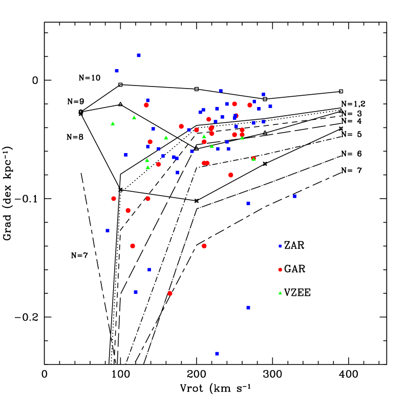
Figure 19: Radial gradients in dex kpc^-1 as obtained from the modeled oxygen abundance radial distributions, computed with a least square straigh line in the radial range $\rm 0.5Rckpc<R<3Rckpc$, as a function of the rotation velocity Vmax in kpc.s^-1. Models are represented by the same line coding than Fig. 10 to 14. Data are from (Zaritsky et al.1994, Garnett et al.1997); van Zee, Salzer & Haynes (1998), shown by squares, dots and triangles, respectively.

Data from (Zaritsky et al.1994, Garnett et al.1997); van Zee, Salzer & Haynes (1998) are over-plotted on this Fig. 19. We see that the modelled trend reproduce the observations, although a more profound analysis about this (and other) correlation will be performed in the future.

4.5 Efficiencies

In order to use this grid for a given galaxy for which observational data are known, we must first select the radial distribution of mass. This means that we must know the total mass, the maximum rotation velocity or, if none of them is available, the luminosity or the magnitude in the I band. According to this value we may choose the number of the distribution from Table 1. Then, 10 different models, corresponding to the 10 different efficiencies, are available.

The standard procedure in chemical evolution would be to see which of them is able to reproduce with success known data such as elemental abundances or gas densities. If more than one observational constraint is available, some kind of minimum error or maximum probability technique may be used for the purpose of choosing the best model. Once this selection is performed we may use the time evolution given by the chosen model to predict the star formation history, the age-metallicity relation, the stellar populations or any other quantity relative to the modelled galaxy. Obviously, the largest the observational number of constraints, the smallest the uncertainty in the selection of the best model. The old and well known uniqueness problem of the chemical evolution suggest that more than one model may reproduce the data. Actually, we have shown in Mollá & Hardy (2002) that this problem reduces greatly when more than two observational constraints can be used. Only 4% of the 500 models computed with with different input parameters could reproduce the observations relative to HI, oxygen abundance and SFR at the same time. Therefore we are confident that models may provide the evolutionary history of a given galaxy within a reasonable accuracy.

Sometimes, however, these observational constraints are not available (or not with sufficient precision) to select the adequate model. In that case, some other method to choose the possible evolutionary track is necessary. Our best models from previous works give us evidence that the efficiencies to form molecular clouds from atomic gas and stars from molecular gas, seem to depend on the galaxy morphological type. If this were the case, the selection of the best model might be easier. In fact, this dependence was already found in Ferrini & Galli (1988); Galli & Ferrini (1989), where these authors quantified the efficiencies to form molecular clouds and the frequency of cloud-cloud collisions, finding that a variation of 10 in the parameters H and $\mu$ is needed when the Hubble type changes from one stage to the next (Sa to Sb, etc..).

Figure 20: a) The efficiency $ln\epsilon_{\mu}$ as a function of the morphological type T represented by $+$ for all galaxies. The solid dots are the averaged values computed with 10 bins. The solid line is a least-square second degree polynomial. b) The efficiency $ln\epsilon_{\mu}$ as a function of $T^{2}$. The solid line is the least-squares straight line.

In order to check if a relation between efficiencies and morphological type exists, we have plotted in Fig. 20, panel a) the logarithmic efficiency $\epsilon_{\mu}$, computed following the equation (19) from section 2.3, as a function of T for the data of Young et al. (1996). There $+$ symbols correspond to the raw values while solid dots represent the averaged values obtained for 10 bins, one for each T. A clear decreasing correlation appears for $T<9$. Values for $T\geq 9$ fall above the trend but the number of points is small for what we assume that the final increase is probably spurious. Based on our previous works, we expect a relation of the form: $\epsilon_{\mu}\propto exp^{-T{2}/A}$. Therefore, in panel b) we have plotted the logarithmic efficiency as a function of $T^{2}$ where a linear correlation is apparent. A least-squares fit gives, for $T<9$ :

$$<ln\epsilon_{\mu}>=-1.60-0.057T^{2},\chi^{2}=1.19$$ (23)

Therefore:

$$<\epsilon_{\mu}>\sim exp^{-T^{2}/20}$$ (24)

On the other hand, taking into account the relationship obtained for the ratio between both efficiencies, $\epsilon_{\mu}$ and $\epsilon_{H}$, this latter one may also be expressed by a similar function : $\epsilon_{H}\propto exp^{-T^{2}/B}$ where B would be 8, following our hypothesis from Section 2.

The result that efficiencies are related to galaxy morphological type may be useful when a model for a given galaxy must be chosen and the observational data are scarce. In that case, once the total mass distribution has been selected from the rotation curve or the luminosity for the galaxy, an initial choice can be made under the assumption that the galaxy evolution is represented by the model of efficiencies N with $N=T$. We warn, however, that given the large dispersion of the data around the averaged efficiency values in Fig. 20, other values of N are also possible.

This finding would imply that the features of spiral galaxies depend at least on two parameters: total mass and morphological type, as some studies about the characteristics of galaxies, as the seminal work by Roberts & Haynes (1994), show (see also Vila-Costas & Edmunds, 1992; , Zaritsky et al.1994, Garnett et al.1997, among those more related with the chemical evolution of galaxies).

It is also well known that the radial gradient, measured as dex $\rm kpc^{-1}$, observed in spiral galaxies depends on morphological type: late-type galaxies show steeper radial distributions of oxygen abundances than earlier ones, which show in some cases almost no gradient (Oey & Kennicutt, 1993; Dutil & Roy, 1999). At the same time, a correlation seems to exist between oxygen abundance and total mass surface density which, in turn, is related to morphological type. This correlation is stronger when the total mass of the galaxy, including the bulge, instead of the mass of the exponential disc alone, is used (Ryder, 1995). It is evident from these works that a linear sequence with the mass can not be obtained, and therefore our models, being a bi-parametric grid, would be adequate to find the best model for each galaxy, although the existing relation between the morphological type of galaxies and their total mass does difficult to discriminate which of these features is the origin of the different evolution of galaxies.

From the chemical evolution point of view, a recent work (Mollá & Márquez, in preparation), where the multiphase evolution model has been applied to a large sample (67) of spiral galaxies, seems to demonstrate that the total mass, through its influence on the collapse time scale, has a larger effect on the evolution of a galaxy and its final radial gradient of abundances than the selected values of the named efficiencies. Thus, it seems as if galaxies would evolve mostly due to their total mass with some dispersion around the mean trend depending on hydrodynamical and environmental characteristics, which are taken into account in some way by the efficiencies values. The morphological type would then be the consequence of the different conditions of the intergalactic medium out of which the galaxy formed.

5 Summary and conclusions

We have calculated the chemical evolution of a wide set of theoretical galaxies characterised by their total mass, through the collapse time scale, and their efficiencies to form molecular clouds and massive stars from cloud-to-cloud collisions.

With the selection of parameters and inputs described above, we have ran a total of 440 models, with 44 different rotation curves –implying 44 values of total mass, characteristic collapse time-scale and disc radius– and 10 sets of efficiencies for each one of them, implying 10 evolutionary rates for the star formation and gas consumption in the disc.

For each model we have obtained the time evolution of the halo and the disc, and therefore the corresponding radial distributions for the relevant quantities (masses, abundances, star formation rate, etc…). The star formation history for each radial region (halo and disc, separately) and within each one, the mass in each phase of matter: diffuse gas, molecular gas, low-mass stars, massive stars and remnants, has been followed. Besides that, we have obtained the abundances of 15 elements: H, D, He3, He4, C12, C13, N14, O16, Ne, Mg, Si, Ca, S, Fe and neutron-rich nuclei, in all radial regions for both halo and disc.

The results of our work can be summarised as follows:

1. The atomic gas shows a maximum in its radial distribution for all galaxies. This maximum is nearer to the galaxy centre in the low mass or less evolved galaxies than in the more evolved or massive galaxies, for which the maximum is along the disc and moving toward the outer zones. This behavior produces, in some cases, a central hole in the distribution of the diffuse gas. The diffuse gas radial distribution results to be a very strong constraint for selecting the best model out of the 10 computed ones with different efficiencies, corresponding to the total mass of a given spiral galaxy.

2. The oxygen abundance reaches a maximum level, as a consequence of a saturation effect which occurs earlier for the massive and more evolved galaxies. The less evolved galaxies do not reach this saturation level, except in the central region, and therefore show a steep radial gradient in their oxygen abundance. The less massive and less evolved galaxies have not yet developed a radial gradient and show flat radial distributions. This simulates an on-off effect: for $N=7$ a radial gradient appears if $\lambda>0.15$ while at $N=8$ it only appears for $\lambda\sim 1.50$. This behavior is in agreement with observations and solves the apparent inconsistency shown by trends showing steep gradients for late type galaxies and flatter ones for the earliest ones, while, at the same time, most irregulars show no gradient at all and very uniform abundances.

3. The model calculated star formation rates reproduce the observed trend between the surface density of this quantity and the total gas density including, not only the massive normal galaxies data, but also the low surface brightness ones.

Actually, to our knowledge, there are not other chemical evolution models which compare predicted with observed radial distributions of diffuse and molecular gas, star formation rate and abundances for disc galaxies other than MWG. In this sense our models should be considered as an improvement over the standard ones.

A study of the possible correlations among galaxy properties and different features obtained from the complete set of results is now possible, since a statistically significant number of theoretical models is available. This requires a deeper analysis which is out of the scope of this paper and will be done in the next future.

Table 5: Model Results: Elemental Abundances.

Time	R	H	D	3He	4He	12C	13C	N	O	Ne	Mg	Si	S	Ca	Fe
…	…	…	…	…	…	…	…	…	…	…	…	…	…	…	…
0.1	14.	0.770	0.70E–04	0.10E–04	0.230	0.11E–06	0.21E–09	0.13E–07	0.92E–06	0.23E–06	0.32E–07	0.55E–07	0.26E–07	0.37E–08	0.42E–07
0.1	12.	0.770	0.70E–04	0.10E–04	0.230	0.12E–06	0.22E–09	0.13E–07	0.95E–06	0.23E–06	0.34E–07	0.57E–07	0.27E–07	0.38E–08	0.44E–07
0.1	10.	0.770	0.70E–04	0.10E–04	0.230	0.13E–06	0.23E–09	0.14E–07	0.10E–05	0.25E–06	0.35E–07	0.60E–07	0.28E–07	0.40E–08	0.46E–07
0.1	8.	0.770	0.70E–04	0.10E–04	0.230	0.14E–06	0.25E–09	0.15E–07	0.11E–05	0.27E–06	0.38E–07	0.65E–07	0.31E–07	0.43E–08	0.50E–07
0.1	6.	0.770	0.70E–04	0.10E–04	0.230	0.15E–06	0.28E–09	0.17E–07	0.12E–05	0.30E–06	0.43E–07	0.73E–07	0.35E–07	0.49E–08	0.56E–07
0.1	4.	0.770	0.70E–04	0.10E–04	0.230	0.18E–06	0.32E–09	0.19E–07	0.14E–05	0.35E–06	0.50E–07	0.85E–07	0.40E–07	0.57E–08	0.65E–07
0.1	2.	0.770	0.70E–04	0.10E–04	0.230	0.45E–06	0.46E–09	0.28E–07	0.38E–05	0.95E–06	0.13E–06	0.22E–06	0.10E–06	0.14E–07	0.15E–06
…	…	…	…	…	…	…	…	…	…	…	…	…	…	…	…
13.2	14.	0.769	0.69E–04	0.12E–04	0.231	0.59E–04	0.12E–06	0.68E–05	0.15E–03	0.34E–04	0.52E–05	0.10E–04	0.50E–05	0.71E–06	0.24E–04
13.2	12.	0.768	0.69E–04	0.13E–04	0.231	0.10E–03	0.21E–06	0.96E–05	0.27E–03	0.57E–04	0.84E–05	0.20E–04	0.96E–05	0.13E–05	0.42E–04
13.2	10.	0.764	0.65E–04	0.21E–04	0.234	0.43E–03	0.98E–06	0.38E–04	0.11E–02	0.21E–03	0.30E–04	0.86E–04	0.40E–04	0.55E–05	0.17E–03
13.2	8.	0.754	0.58E–04	0.44E–04	0.240	0.11E–02	0.44E–05	0.16E–03	0.28E–02	0.54E–03	0.76E–04	0.22E–03	0.10E–03	0.14E–04	0.44E–03
13.2	6.	0.746	0.51E–04	0.73E–04	0.246	0.16E–02	0.11E–04	0.37E–03	0.40E–02	0.78E–03	0.11E–03	0.33E–03	0.16E–03	0.21E–04	0.67E–03
13.2	4.	0.736	0.43E–04	0.13E–03	0.253	0.21E–02	0.22E–04	0.64E–03	0.49E–02	0.98E–03	0.14E–03	0.44E–03	0.21E–03	0.28E–04	0.93E–03
13.2	2.	0.693	0.63E–05	0.43E–03	0.287	0.37E–02	0.71E–04	0.18E–02	0.81E–02	0.18E–02	0.26E–03	0.83E–03	0.40E–03	0.56E–04	0.20E–02

References

- Adler & Liszt (1989) Adler, D. S. & Liszt, H. S., 1989, ApJ, 339, 836
- (2) Afflerbach, A., Churchwell, E., & Werner, M. W., 1997, ApJ, 478, 190
- Allende Prieto et al. (2002) Allende Prieto, C., Lambert, D. L., & Asplund, M., 2002, ApJL, 573, L137
- Allende Prieto et al. (2001) Allende Prieto, C., Barklem, P. S., Asplund, M., & Ruiz Cobo, B., 2001, ApJ, 558, 830
- (5) Allende Prieto, C., Lambert, D. L., & Asplund, M., 2001, ApJL, 556, L63
- Barry (1988) Barry, D. C., 1988, ApJ, 334, 436
- Beauchamp & Hardy (1997) Beauchamp, D., & Hardy, E., 1997, AJ, 113, 1666
- Belley & Roy (1992) Belley, J. & Roy, J., 1992, ApJS, 78, 61
- Bergin et al. (2004) Bergin E. A., Hartmann L. W., Raymond J. C., Ballesteros-Paredes J., 2004, ApJ, 612, 921
- Boissier & Prantzos (2000) Boissier, S. & Prantzos, N., 2000, MNRAS, 312, 398
- (11) Boissier, S., Boselli, A., Prantzos, N., & Gavazzi, G., 2001, MNRAS., 321, 733
- Braun (2001) Braun, J. M., 2001, Dwarf Galaxies and their Environment, Proceedings of the Bonn/Bochum-Graduiertenkolleg International Conference, Germany, 23-27 January 2001, Eds.: de Boer K.S., Dettmar R.-J., Klein U., Shaker Verlag, p. 5
- Broeils & Rhee (1997) Broeils A. H., Rhee M.-H., 1997, A&A, 324, 877
- (14) Bronfman, L., Cohen, R. S., Alvarez, H., et al., 1988, ApJ, 324, 248
- (15) Bronfman, L., Casassus, S., May, J., & Nyman, L.-Å., 2000, A&A, 358, 521
- Burstein & Rubin (1985) Burstein D., Rubin V. C., 1985, ApJ, 297, 423
- Campos-Aguilar, Prieto, & García (1993) Campos-Aguilar A., Prieto M., García C., 1993, A&A, 276, 16
- (18) Carignan, C., Charbonneau, P., Boulanger, F., & Viallefond, F., 1990, A&A, 234, 43
- Carraro, Ng, & Portinari (1998) Carraro, G., Ng, Y. K., & Portinari, L. 1998, MNRAS, 296, 1045
- Case & Bhattacharya (1996) Case G., Bhattacharya D., 1996, A&AS, 120, 437
- Castellanos et al. (2002) Castellanos, M., Díaz, A. I., & Terlevich, E., 2002, MNRAS, 329, 315
- (22) Cayatte, V., van Gorkom, J. H., Balkowski, C., & Kotanyi, C., 1990, AJ, 100, 604
- (23) Chang R. X., Hou J. L., Shu C. G., Fu C. Q., 1999, A&A, 350, 38
- (24) Chiappini C., Matteucci F., Beers T. C., Nomoto K., 1999, ApJ, 515, 226
- Christensen et al. (1997) Christensen, T., Petersen, L., & Gammelgaard, P., 1997, A&A, 322, 41
- Cimatti et al. (2002) Cimatti A., et al., 2002, A&A, 391, L1
- Cimatti et al. (2004) Cimatti A., et al., 2004, Natur, 430, 184
- Clayton (1987) Clayton, D. D., 1987, ApJ, 315, 451
- Clayton (1988) Clayton, D. D., 1988, MNRAS, 234, 1
- Corbelli & Salucci (2000) Corbelli, E. & Salucci, P., 2000, MNRAS, 311, 441.
- de Blok & McGaugh (1996) de Blok, W. J. G. & McGaugh, S. S., 1996, ApJL, 469, L89
- Degioia-Eastwood et al. (1984) Degioia-Eastwood K., Grasdalen G. L., Strom S. E., Strom K. M., 1984, ApJ, 278, 564
- (33) Deharveng, L., Caplan, J., Lequeux, J., Azzopardi, M., Breysacher, J., Tarenghi, M., & Westerlund, B., 1988, A&AS, 73, 407
- Diaz (1989) Diaz A. I., 1989, in Evolutionary phenomena in galaxies. Cambridge and New York, Cambridge University Press, p. 377-397.
- Díaz et al. (2000) Díaz, A. I., Castellanos, M., Terlevich, E., & García-Vargas, M. L., 2000 MNRAS, 318, 462
- Domínguez-Tenreiro, Sáiz, & Serna (2004) Domínguez-Tenreiro R., Sáiz A., Serna A., 2004, ApJ, 611, L5
- Dutil & Roy (1999) Dutil, I., & Roy, J.-R., 1999, ApJ, 516, 62
- Edmunds & Roy (1993) Edmunds M. G., Roy J., 1993, MNRAS, 261, L17
- Edvardsson et al. (1993) Edvardsson, B., Andersen, J., Gustafsson, B., Lambert, D. L., Nissen, P. E., & Tomkin, J., 1993, A&A, 275, 101
- Eggen, Lynden-Bell, & Sandage (1962) Eggen O. J., Lynden-Bell D., Sandage A. R., 1962, ApJ, 136, 748
- Esteban, Peimbert, Torres-Peimbert, & García-Rojas (1999c) Esteban, C., Peimbert, M., Torres-Peimbert, S., & García-Rojas, J., 1999c, Revista Mexicana de Astronomía y Astrofísica, 35, 65
- Esteban, Peimbert, & Torres-Peimbert (1999b) Esteban, C., Peimbert, M., & Torres-Peimbert, S. 1999b, A&A, 342, L37
- Esteban et al. (1999) Esteban, C., Peimbert, M., Torres-Peimbert, S., García-Rojas, J., & Rodríguez, M. 1999a, ApJS, 120, 113
- Ferrini & Galli (1988) Ferrini, F. & Galli, D., 1988, A&A, 195, 27
- Ferrini et al. (1992) Ferrini F., Matteucci F., Pardi C., Penco U., 1992, ApJ, 387, 138
- (46) Ferrini, F., Mollá, M., Pardi, C., & Díaz, A. I., 1994, ApJ, 427, 745
- Ferrini, Palla & Penco (1990) Ferrini, F., Palla F., & Penco, U., 1990, A&A, 213, 3
- Fich & Silkey (1991) Fich, M. & Silkey, M., 1991, ApJ, 366, 107
- (49) Fitzsimmons, A., Dufton, P.L. & Rolleston, W.R.J., 1992, MNRAS, 259, 489
- Friedli, Benz, & Kennicutt (1994) Friedli D., Benz W., Kennicutt R., 1994, ApJ, 430, L105
- (51) Gallagher, J. S., Hunter, D. A., & Tutukov, A. V., 1984, ApJ, 284, 544
- Galli & Ferrini (1989) Galli, D. & Ferrini, F., 1988, A&A, 218, 31
- (53) Garnett, D. R., Shields, G. A., Skillman, E. D., Sagan, S. P., & Dufour, R. J., 1997, ApJ, 489, 63
- Garnett (1998) Garnett D. R., 1998, RMxAC, 7, 58
- Garnett, Kennicutt, & Bresolin (2004) Garnett D. R., Kennicutt R. C., Bresolin F., 2004, ApJ, 607, L21
- Garwood & Dickey (1989) Garwood, R.W. & Dickey, J.M., 1989, ApJ, 338, 41
- Gavilán et al. (2004) Gavilán, M., Buell, J. F. & Mollá, M., 2004, A&A, in press
- Gavilán & Mollá (2004b) Gavilán, & Mollá, M., 2004, in The Many Scales of the Universe: JENAM 2004 Astrophysics Review, Eds. J.C. del Toro et al., (Springer Academic Pub.: Dordrecht, Netherlands), in press.
- Glazebrook et al. (2004) Glazebrook K., et al., 2004, Nature, 430, 181
- (60) Goudfrooij P., Gorgas J., Jablonka P., 1999, Ap&SS, 269, 109
- (61) Grabelsky, D.A., Cohen, R.S. & Bronfmann, L., 1987, ApJ, 315, 122
- Graham & de Block (2001) Graham, A.W. & de Block, W.J.G., 2001, ApJ, 556, 177
- Grevesse & Sauval (1998) Grevesse, N. & Sauval, A. J., 1998, Space Science Reviews, 85, 161
- Güsten & Mezger (1983) Güsten,R. & Mezger, P.G., 1983, Vistas in Astronomy, 26, 159
- (65) Guzmán, R., Koo, D. C., Faber, S.M., et al., 1996, ApJ, 460, L5
- Heavens et al. (2004) Heavens A., Panter B., Jimenez R., Dunlop J., 2004, Nature, 428, 625
- Henry & Worthey (1999) Henry, R. C. B. & Worthey, G., 1999, PASP, 111, 919
- (68) Heyer, M. H., Corbelli, E., Schneider, S. E., & Young, J. S., 2004, ApJ, 602, 723
- Holweger (2001) Holweger, H., 2001, AIP Conf. Proc. 598: Joint SOHO/ACE workshop ”Solar and Galactic Composition”, 23
- (70) Iwamoto, K., Brachwiz, F., Nomoto, K. et al., 1999, ApJSS, 125, 439
- (71) Jimenez, R. Panter, B., Heavens, A., & Verde, L., 2004, MNRAS, submitted (astro-ph/0403294)
- Kenney & Young (1989) Kenney, J. D., & Young, J. S., 1989, ApJ, 344, 171
- Kennicutt (1989) Kennicutt, R. C.,Jr., 1989, ApJ, 344, 685
- Kennicutt (1998) Kennicutt R. C., 1998, ApJ, 498, 541
- Kennicutt & Garnett (1996) Kennicutt, R. C., Jr. & Garnett, D.R., 1996, Ap.J., 456, 518
- Kennicutt, Bresolin, & Garnett (2003) Kennicutt R. C., Bresolin F., Garnett D. R., 2003, ApJ, 591, 801
- Klessen (2001) Klessen, R. S., 2001, ApJ, 556, 837
- Kobulnicky (1998) Kobulnicky H. A., 1998, ASP.Conf.Series 147, 108
- Kotoneva et al. (2002) Kotoneva E., Flynn C., Chiappini C., Matteucci F., 2002, MNRAS, 336, 879
- Kroupa (2001) Kroupa, P., 2001, MNRAS, 322, 231
- Kwitter & Aller (1981) Kwitter, K. B. & Aller, L. H., 1981, MNRAS, 195, 939.
- Lacey & Fall (1985) Lacey, C. G. & Fall, S. M., 1985, ApJ, 290, 154
- Lelièvre & Roy (2000) Lelièvre, M. , Roy, J., 2000, AJ, 120, 1306
- Legrand (2000) Legrand, F., 2000, A&A, 354, 504
- Lequeux (1983) Lequeux J., 1983, A&A, 125, 394
- Lynden-Bell (1975) Lynden-Bell, D., 1975, Vistas in Astronomy, 19, 299
- Martin & Kennicutt (2001) Martin, C. L. & Kennicutt, R. C., 2001, ApJ, 555, 301
- Martin & Roy (1994) Martin, P. & Roy, J., 1994, ApJ, 424, 599
- Matteucci (1992) Matteucci, F. 1992, Memorie della Societa Astronomica Italiana, 63, 301
- Matteucci et al. (1998) Matteucci, F., Ponzone, R., & Gibson, B. K. 1998, A&A, 335, 855
- McCall et al. (1985) McCall, M. L., Rybsky, P. M., & Shields, G. A., 1985, ApJS, 57, 1
- McCarthy et al. (2004) McCarthy P. J., et al., 2004, ApJ, 614, L9
- Meyer et al. (2000) Meyer, M. R., Adams, F. C., Hillebrandt, L. A., Carpenter, J. M., & Larson, R. B., 2000, in Protostars & Planets IV, Eds. Manning, V., Boss, A. P., & Russell, S. S. (Tucson: the University of Arizona Press), p.121
- Meyer, Jura & Cardelli (1998) Meyer, D. M., Jura, M., & Cardelli, J. A., 1998, ApJ, 493, 222
- Meyer, Cardelli & Sofia (1997) Meyer, D. M., Cardelli, J. A., & Sofia, U. J., 1997, ApJL, 490, L103
- Mirabel (1989) Mirabel, I. F., 1989, IAU Colloq. 120: Structure and Dynamics of the Interstellar Medium, 396
- Mollá & Ferrini (1995) Mollá, M., Ferrini, F., 1995, ApJ, 454,726
- Mollá et al. (1996) Mollá, M., Ferrini, F., & Díaz, A. I., 1996, ApJ, 466, 668
- (99) Mollá, M., Hardy, E., & Beauchamp, D., 1999, ApJ, 513, 695
- Mollá & Roy (1999) Mollá, M., Roy, J.-R., 1999, ApJ, 514, 781
- Mollá & Roy (1999b) Mollá, M., & Roy, J.-R., 1999, in Chemical Evolution from zero to high redshift, Eds. J.R. Walsh & M. R. Rosa (Springer-Verlag: Berlín), 155
- (102) Mollá, M., Ferrini, F., & Gozzi, G., 2000, MNRAS, 316, 345.
- Mollá & Hardy (2002) Mollá, M. & Hardy, E., 2002, AJ, 123, 3055
- Moos et al. (2002) Moos, H. W. et al., 2002, ApJS, 140, 3
- Nakanishi & Sofue (2004) Nakanishi, H. & Sofue, Y., 2004, PASJ, 55, 191
- Newton (1980) Newton K., 1980, MNRAS, 190, 689
- Nishiyama & Nakai (2001) Nishiyama, K. & Nakai, N., 2001, PASJ, 53, 713
- (108) Nomoto, K., Thielemann, F. K., & Yokoi, K., 1984, ApJ, 286, 644
- Oey & Kennicutt (1993) Oey, M. S., & Kennicutt, R. C., 1993, ApJ, 411, 137
- (110) Pagel,B. E. J., Edmunds, M. G., Blackwell, D. E., Chun, M. S., & Smith, G., 1979, MNRAS, 189, 95
- Palla (2004) Palla F., 2004, BaltA, 13, 349
- Palunas & Williams (2000) Palunas, P. & Williams, T.B., 2000, AJ, 120, 2884
- Pardi & Ferrini (1994) Pardi M. C., Ferrini F., 1994, ApJ, 421, 491
- Parravano (1990) Parravano, A., 1989, ApJ, 347, 812
- Peimbert (1979) Peimbert, M., 1979, IAU Symp. 84: The Large-Scale Characteristics of the Galaxy, 84, 307
- Peimbert (1999) Peimbert, M., 1999, Chemical Evolution from Zero to High Redshift, 30
- Persic et al. (1996) Persic, M., Salucci, P. & Steel, F., 1996, MNRAS, 281, 27, (PSS)
- Pilyugin (2001) Pilyugin, L. S., 2001, A&A, 369, 594
- Pilyugin (2000) Pilyugin, L. S., 2000, A&A, 362, 325
- Portinari & Chiosi (1999) Portinari, L. & Chiosi,C., 1999, A&A, 350, 827
- Portinari, Chiosi, & Bressan (1998) Portinari L., Chiosi C., Bressan A., 1998, A&A, 334, 505
- Prantzos & Boissier (2000) Prantzos, N. & Boissier, S., 2000, MNRAS, 313, 338
- Pringle, Allen, & Lubow (2001) Pringle J. E., Allen R. J. & Lubow S. H., 2001, MNRAS, 327, 663
- Proctor & Sansom (2002) Proctor R. N., Sansom A. E., 2002, MNRAS, 333, 517
- Puche, Carignan, & Bosma (1990) Puche, D., Carignan, C., & Bosma, A., 1990, AJ, 100, 1468.
- Rana (1991) Rana, N. C., 1991, ARA&A, 29, 129
- Reddy, Tomkin, Lambert, & Allende Prieto (2003) Reddy, B. E., Tomkin, J., Lambert, D. L., & Allende Prieto, C., 2003, MNRAS, 340, 304
- Regan et al. (2001) Regan M. W., Thornley M. D., Helfer T. T., Sheth K., Wong T., Vogel S. N., Blitz L., Bock D. C.-J., 2001, ApJ, 561, 218
- Rhee & van Albada (1996) Rhee M.-H., van Albada T. S., 1996, A&AS, 115, 407
- Roberts & Haynes (1994) Roberts, M. S. & Haynes, M. P., 1994, ARA&A., 32, 115
- (131) Rocha-Pinto, H. J., Scalo, J., Maciel, W. J., & Flynn, C., 2000, A&A, 358, 869.
- (132) Rocha-Pinto, H. J., Maciel, W. J., Scalo, J., & Flynn, C., 2000, A&A, 358, 850.
- (133) Rogstad, D. H., Chu, K., & Crutcher, R. M. 1979, ApJ, 229, 509
- Rownd & Young (1999) Rownd B. K., Young J. S., 1999, AJ, 118, 670
- Roy (1996) Roy, J.-R., 1996, ASP Conf. Ser. 91: IAU Colloq. 157: Barred Galaxies, 63
- Roy, Belley, Dutil, & Martin (1996) Roy, J., Belley, J., Dutil, Y., & Martin, P., 1996, ApJ, 460, 284
- Rumstay & Kaufman (1983) Rumstay K. S., Kaufman M., 1983, ApJ, 274, 611
- Ryder (1995) Ryder, S. D., 1995, ApJ, 444, 610
- Sage & Solomon (1989) Sage, L. J. & Solomon, P. M., 1989, ApJL, 342, L15
- Sáiz, Domínguez-Tenreiro, & Serna (2004) Sáiz A., Domínguez-Tenreiro R., Serna A., 2004, ApJ, 601, L131
- (141) Samland, M., Hensler, G. & Theis, Ch., 1997, ApJ, 476, 544
- (142) Sancisi,R., Fraternali, F., Oosterloo, T., van Moorsel, G., 2001, ASP. Conf. Series, Vo. 230, 111 Eds.J.E.Hibbard, M.P. Rupen and J.H. van Gorkom
- Sandage (1987) Sandage, A., 1987, AJ, 93, 610
- Scalo (1998) Scalo, J., 1998, ASP Conf. Ser. 142: The Stellar Initial Mass Function (38th Herstmonceux Conference), Eds. Gilmore, G. & Howell, D. (San Francisco: ASP), 201.
- Scalo (1986) Scalo J. M., 1986, Fund. of Cosmic Phys., 11, 1
- Sellwood & Kosowsky (2000) Sellwood, J. A. & Kosowsky, A., 2001, ASP. Conf. Series, Vol. 230, Eds.J.E.Hibbard, M.P. Rupen and J.H. van Gorkom
- Shaver et al. (1983) Shaver, P. A.,McGee, R. X., Newton, L. M., Danks, A. C., & Pottasch, S. R., 1983, MNRAS, 204, 53
- Simien & de Vaucouleurs (1986) Simien, F. & de Vaucouleurs, G., 1986, ApJ, 302, 564
- Smartt & Rolleston. (1997) Smartt, S. J. & Rolleston, W. R. J., 1997, ApJL, 481, L47
- Smartt et al. (2001) Smartt, S. J., Venn, K. A., Dufton, P. L., Lennon, D. J., Rolleston, W. R. J., & Keenan, F. P., 2001, A&A 367, 86
- Sofia et al. (2001) Sofia, U. J. & Meyer, D. M., 2001, ApJL, 554, L221
- Sommer-Larsen & Yoshii (1989) Sommer-Larsen, J. & Yoshii, Y., 1989, MNRAS, 238, 133
- Strong et al. (2004) Strong A. W., Moskalenko I. V., Reimer O., Digel S., Diehl R., 2004, A&A, 422, L47
- Tacconi & Young (1989) Tacconi L. J., Young J. S., 1989, ApJS, 71, 455
- Talbot (1980) Talbot, R. J., 1980, ApJ, 235, 821
- Tinsley (1980) Tinsley, B.M., 1980, Fund. Cosmic. Phys., 5, 287
- Twarog (1980) Twarog, B. A., 1980, ApJ, 242, 242
- Tully (1988) Tully, R.B., 1988, Nearby Galaxies Catalog, Cambridge University Press,Cambridge
- Tully & Pierce (2000) Tully, R. B. & Pierce, M. J., 2000, ApJ, 533, 744
- (160) Valle, G., Ferrini, F., Galli, D. & Shore, S.N., 2002, ApJ, 566, 252
- Vallenari, Bertelli, & Schmidtobreick (2000) Vallenari A., Bertelli G., Schmidtobreick L., 2000, A&A, 361, 73
- van den Hoek et al. (2000) van den Hoek, L. B., de Blok, W. J. G., van der Hulst, J. M., & de Jong, T., 2000, A&A, 357, 397
- van Zee, Salzer & Haynes (1998) van Zee, L., Salzer, J. J., Haynes, M. P., O’Donoghue, A. A., & Balonek, T. J., 1998, AJ, 116, 2805.
- Verter & Hodge (1995) Verter,F., & Hodge, P., 1995, ApJ, 446, 616
- Vila-Costas & Edmunds (1992) Vila-Costas, B., & Edmunds, M. G., 1992, MNRAS, 259, 121
- Vílchez et al. (1988) Vílchez, J. M., Pagel, B. E. J., Díaz, A. I., Terlevich, E., & Edmunds, M. G., 1988, MNRAS, 235, 633.
- Vílchez & Esteban (1996) Vílchez, J. M. & Esteban, C., 1996, MNRAS, 280, 720
- Walsh et al. ( 2002) Walsh W., Beck R., Thuma G., Weiss A., Wielebinski R., Dumke M., 200 2, A&A, 388, 7
- Walsh & Roy (1997) Walsh J. R., Roy J.-R., 1997, MNRAS, 288, 726
- Warmels (1988) Warmels R. H., 1988, A&AS, 72, 427
- Wevers, van der Kruit & Allen (1986) Wevers, B. M. H. R., van der Kruit, P. C., & Allen, R. J., 1986, A&AS, 66, 505
- Wilson (1995) Wilson, C. D., 1995, ApJ, 448, L97
- Williams & McKee (1997) Williams J. P., McKee C. F., 1997, ApJ, 476, 166
- Wyse (1997) Wyse, R. F. G., 1997, ApJ, 490, L69
- Woosley & Weaver (1995) Woosley, S. E. & Weaver, T. A., 1995, ApJS , 101, 181
- (176) Wouterlook, J.G.A., Brand, J., Burton, W.B. & Kwee, K. K., 1990, A&A, 230, 21
- Young et al. (1996) Young J. S., Allen L., Kenney J. D. P., Lesser A., Rownd B., 1996, AJ, 112, 1903
- (178) Zaritsky, D., Kennicutt, R. C., & Huchra, J. P., 1994, ApJ , 420, 87