Galaxy clustering constraints on deviations from Newtonian gravity at cosmological scales

Abstract

In spite of the growing observational evidence for dark matter and dark energy in the universe, their physical nature is largely unknown. In fact, several authors have proposed modifications of Newton’s law of gravity at cosmological scales to account for the apparent acceleration of the cosmic expansion. Inspired by such suggestions, we attempt to constrain possible deviations from Newtonian gravity by means of the clustering of SDSS (Sloan Digital Sky Survey) galaxies. To be specific, we assume a simple modification of Newton’s law with an additional Yukawa-type term characterized by the amplitude $\alpha$ and the length scale $\lambda$. Adopting spatially-flat universes dominated by cold dark matter and/or dark energy, we solve a linear perturbation equation for the growth of density fluctuations. In particular, we find an exact analytic solution for the Einstein – de Sitter case. Following the Peacock-Dodds prescription, we compute the nonlinear power spectra of mass fluctuations, perform a statistical comparison with the SDSS galaxy data, and derive constraints in the $\alpha$-$\lambda$ plane; for instance, we obtain the constraints of $-0.5<\alpha<0.6$ and $-0.8<\alpha<0.9$ (99.7% confidence level) for $\lambda=5h^{-1}$Mpc and $10h^{-1}$Mpc, respectively. We also discuss several future possibilities for improving our analysis.

I Introduction

Recent observations on cosmological scales suggest the presence of a non-zero cosmological constant or dark energy in the universe. Adopting spatially-flat Friedmann-Robertson-Walker (FRW) models, type Ia supernovae Knop:2003iy and cosmic microwave background (CMB) data Bennett:2003bz ; Spergel:2003cb are simultaneously well fit by $\Omega_{\Lambda}\approx 0.7$ and $\Omega_{\rm m}\approx 0.3$, where $\Omega_{\Lambda}$ and $\Omega_{\rm m}$ denote the dimensionless cosmological constant and the density parameter of non-relativistic matter, respectively. In fact, nearly all the available observational data are in good agreement with the above model parameters.

On the other hand, the physical origin and nature of such dark energy components remain to be understood. In this paper we will consider a possible deviation from Newton’s law of gravity that are motivated by recent proposals for an alternative to dark energy Dvali:2000hr ; Deffayet:2000uy or as a possible consequence of dark energy Sealfon ; Nusser04 ; Farrar-Peebles . While this idea seems exotic, the validity of Newton’s law has not been demonstrated rigorously on cosmological scales Adelberger:2003zx ; Hoyle:2004cw . In addition, the presence of dark energy in the standard FRW model is equivalent to introducing a repulsive force in the cosmic expansion. In a sense, this is equivalent to changing Newton’s law of gravity on cosmological scales by modifying the matter content of the universe. The idea behind this paper is to explore observable consequences of a modification of gravity itself. We note that in retrospect this is closer to Einstein’s original idea in introducing the cosmological constant; he introduced the $\Lambda$-term on the left-hand side of the field equation. Nowadays this term is usually interpreted as an additional term in the energy-momentum tensor on the right-hand side.

While our current approach is entirely empirical, there have been several specific attempts to construct self-consistent cosmological models including deviations from Newton’s law on cosmological scales. For instance, Dvali, Gabadadze and Porrati proposed a scenario (DGP model, hereafter) Dvali:2000hr ; Deffayet:2000uy to explain the accelerating universe as a result of gravity leaking into extra dimensions in the context of a braneworld model. According to the DGP model, the accelerating universe is naturally explained without dark energy component, but rather by the modification of Newton’s law of gravity on cosmological scales. A variety of astrophysical and cosmological consequences of the DGP model were discussed by several authors Deffayet:2001pu ; Lue:2004rj ; Alcaniz:2004kq ; Lue:2004za . Other proposals which suggest deviations from Newton gravity on very large scales include a “ghost condensation” model Arkani-Hamed:2003uy ; Arkani-Hamed:2003uz .

We would like to derive constraints on deviations from Newton’s law that are independent of any specific models to the extent possible. Thus, we adopt an empirical parameterization of the deviation from Newton’s law over $10\sim 100$ Mpc scales while the cosmic expansion is assumed to exactly follow that of the standard FRW model.

Note that, strictly speaking, our approach is not fully self-consistent in that our modified gravity law has an effective gravitational constant $G_{\rm eff}=G_{\rm N}(1+\alpha)$ asymptotically in the large-scale limit, but we still assume that the cosmic expansion follows the standard FRW cosmology with $G_{\rm N}$. As discussed below, however, this does not significantly change our conclusions.

Sealfon et al. Sealfon recently carried out a similar analysis in the same spirit. They derive linear theory predictions for the matter power spectrum in modified gravity models and obtain constraints on deviations from the inverse-square law using 2dF (Two-degree Field) and SDSS (Sloan Digital Sky Survey) galaxy data. Our paper differs from theirs in the following three respects: (a) We do not assume a priori that any fractional deviation from Newton’s law is small. The analysis of Sealfon et al. is applicable only in a perturbative regime (i.e., $\alpha\ll 1$). (b) Sealfon et al. solved the linear perturbation equation for the growth of density fluctuations assuming an incorrect scaling between wave-number and the scale factor. We, however, solve the original perturbation equation without such a scaling assumption. Finally (c) we take into account gravitational non-linearity by applying the Peacock-Dodds prescription Peacock:1996ci . As a result, we believe that the constraints in our paper are more reliable.

The rest of the paper is organized as follows. Section II describes our models for modified gravity. In Sec. III we solve the linear perturbation equation for density fluctuations in modified gravity models, and the nonlinear power spectra are computed in Sec. IV by applying the Peacock-Dodds prescription. Section V compares these theoretical predictions with the observed power spectrum of SDSS galaxies. Finally Sec. VI is devoted to conclusions and discussion.

II Model Assumptions

The basic equation that we solve in this paper is

$$\ddot{\delta}+2H(t)\dot{\delta}-\Delta_{\bm{r}}\Phi=0,$$ (1)

where

$$\delta(\bm{r},t)\equiv\frac{\rho(\bm{r},t)-\bar{\rho}(t)}{\bar{\rho}(t)}$$ (2)

is a fractional mass density fluctuation, $\bar{\rho}(t)$ is the mean mass density, $H(t)$ is the Hubble parameter, $\Phi$ is the modified Newtonian potential and $\bm{r}$ is a proper coordinate. The dot denotes the derivative with respect to the cosmic time $t$. To solve equation (1) one has to specify the functional form of $H(t)$ and $\Phi$. In addition, we will confront theoretical predictions against the observed power spectrum of SDSS galaxies. Thus we need an additional assumption of the spatial biasing of SDSS galaxies with respect to the underlying dark matter. We adopt the following four major assumptions in performing the analysis.

(i) For the gravitational potential $\Phi$, we consider two models. The first (Model I) is to simply change the amplitude of Newton’s constant, $G_{\rm N}$:

$$\Phi(\bm{r})=-G_{\rm N}(1+\alpha_{0})\int dr^{\prime 3}\frac{\rho(\bm{r}^{\prime})}{|\bm{r}-\bm{r}^{\prime}|},$$ (3)

where $\alpha_{0}$ is a scale-independent parameter characterizing the deviation. The effective gravitational constant in this model is simply $G_{\rm eff}=G_{\rm N}(1+\alpha_{0})$. While this simple model is useful in understanding a basic outcome of modified gravitational theories, it may be inconsistent with precise tests of Newton’s gravity on small scales. Therefore we also consider another model (Model II) where the deviation is restricted to scales larger than $\lambda$:

$$\Phi(\bm{r})=-G_{\rm N}\int dr^{\prime 3}\frac{\rho(\bm{r}^{\prime})}{|\bm{r}-\bm{r}^{\prime}|}\left[1+\alpha\left(1-e^{-\frac{|\bm{r}-\bm{r}^{\prime}|}{\lambda}}\right)\right].$$ (4)

Note that $\lambda$ is defined in proper, rather than comoving, length, and we consider $1h^{-1}\text{Mpc}\leq\lambda\leq 30h^{-1}\text{Mpc}$ below. Equation (4) recovers the conventional Newton potential for $r\ll\lambda$, and asymptotically approaches Model I with $G_{\rm eff}=G_{\rm N}(1+\alpha)$ for $r\gg\lambda$. The transition between these two regimes is described by the Yukawa-like term but our result below is insensitive to that particular choice.

(ii) We assume that general relativity is valid on the horizon scale, i.e., that the cosmic expansion is described by the standard FRW model. Strictly speaking, this assumption may not be fully consistent with our modified gravity law on local scales (Models I and II). However, our primary interest in this paper is the matter clustering on scales of $1h^{-1}\text{Mpc}\leq\lambda\leq 30h^{-1}\text{Mpc}$, which should not be affected by evolution of structure on much larger scales that are in the linear regime. In other words, even if we introduced another cutoff in Model II so as to recover the Newton gravity at scales $\gg 100h^{-1}\text{Mpc}$, our results would hardly be affected. This explains why we use the FRW model in describing the cosmic expansion while non-Newtonian gravity controls the dark matter clustering. For the same reason, we assume that our modification of gravity does not change the angular power spectrum of the CMB.

In reality, we do not necessarily have to assume the validity of general relativity on horizon scales; the unperturbed model could differ from general relativity and still be consistent with observations. We will defer exploring such possibilities for now and adopt this assumption just for simplicity throughout the present analysis.

(iii) In addition, we assume that the universe is dominated by cold dark matter (CDM) and/or the cosmological constant. To be specific, we consider two spatially flat models with and without the cosmological constant: $\Omega_{\rm m}+\Omega_{\Lambda}=1$ (Table I). Hence we use the conventional models for the Hubble parameter $H$ in equation (1) and the matter transfer function Eisenstein:1997ik .

Table 1: Parameters of cosmological models

Model	$\Omega_{\rm m}$	$\Omega_{\Lambda}$	$\Omega_{\rm b}$	$h$	$\sigma_{8}$
$\Lambda$-CDM	0.3	0.7	0.04	0.7	0.9
EdS-CDM	1.0	0.0	0.04	0.7	0.6

(iv) Finally, we assume that SDSS galaxies are fair tracers of the total mass distribution, but allow for a scale-independent linear bias, $b_{*}$, for $L_{*}$ galaxies. We use the power spectrum of SDSS galaxies, $P_{\rm gg}(k;L_{*})$, which is corrected for luminosity-dependent bias and refers to the clustering of $L_{*}$ galaxies Tegmark . Then we attempt to constrain the parameter space of $\alpha$ and $\lambda$ ($\alpha_{0}$ in Model I) by fitting to

$$P_{\rm gg}(k;L_{*})=b_{*}^{2}P_{\text{\rm mass}}(k;\alpha,\lambda).$$ (5)

The scale independence of the biasing parameter is a fairly conventional assumption in the linear regime where the growth rate is scale independent. Note, however, that our Model II evolves in a weakly scale-dependent fashion even in linear theory (see Fig. 2 below). Nevertheless we assume that $b_{*}$ is independent of $k$ for simplicity.

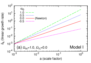
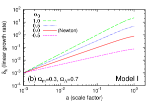
Figure 1: Linear growth rate in Model I where $G_{\rm eff}=(1+\alpha_{0})G_{\rm N}$ is independent of scale; (a) $\Omega_{\rm m}=1$ and $\Omega_{\Lambda}=0$, (b) $\Omega_{\rm m}=0.3$ and $\Omega_{\Lambda}=0.7$.

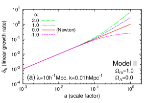
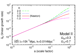
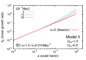
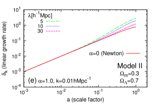
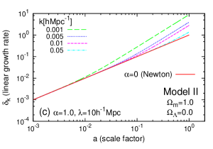
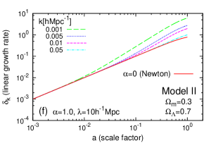
Figure 2: Linear growth rate in Model II; (a) $\alpha$-dependence for $\lambda=10h^{-1}$Mpc and $k=0.01h$Mpc^-1 ($\Omega_{\rm m}=1$ and $\Omega_{\Lambda}=0$), (b) $\lambda$-dependence for $\alpha=1$ and $k=0.01h$Mpc^-1 ($\Omega_{\rm m}=1$ and $\Omega_{\Lambda}=0$), (c) $k$-dependence for $\alpha=1$ and $\lambda=10h^{-1}$Mpc ($\Omega_{\rm m}=1$ and $\Omega_{\Lambda}=0$), (d) $\alpha$-dependence for $\lambda=10h^{-1}$Mpc and $k=0.01h$Mpc^-1 ($\Omega_{\rm m}=0.3$ and $\Omega_{\Lambda}=0.7$), (e) $\lambda$-dependence for $\alpha=1$ and $k=0.01h$Mpc^-1 ($\Omega_{\rm m}=0.3$ and $\Omega_{\Lambda}=0.7$), (f) $k$-dependence for $\alpha=1$ and $\lambda=10h^{-1}$Mpc ($\Omega_{\rm m}=0.3$ and $\Omega_{\Lambda}=0.7$). In all the panels, the results for $\alpha=0$ (Newton’s law of gravity) are plotted in solid curves for reference.

III Linear perturbation theory

In this section, we focus on linear evolution of density fluctuation and solve Eq. (1) for the two models. Let us begin with Model I. In this case, the Fourier transform of Eq. (3) in the comoving coordinate yields

$$\left[\Delta_{\bm{x}}\Phi(\bm{x})\right]_{\bm{k}}=4\pi Ga^{2}\bar{\rho}\left(1+\alpha_{0}\right)\delta_{\bm{k}},$$ (6)

where $a$ is the scale factor (normalized to unity at $z=0$) and $\delta_{\bm{k}}$ denotes the Fourier transform of $\delta$. Note that $\bm{x}$ is the comoving coordinate and we define $\bm{k}$ as the comoving wave-number.

Substituting Eq. (6) into Eq. (1), we obtain

$$\ddot{\delta}_{\bm{k}}+2H\dot{\delta}_{\bm{k}}-\frac{3}{2}(1+\alpha_{0})\left(1-\frac{H_{0}^{2}\Omega_{\Lambda}}{H^{2}}\right)H^{2}\delta_{\bm{k}}=0$$ (7)

in spatially flat models, where $H_{0}$ is the Hubble constant at the present.

In particular, we find that Eq. (7) has an analytic solution in the Einstein-de Sitter model:

$$\delta_{\bm{k}}\propto a^{-\frac{1}{4}\pm\frac{\sqrt{1+24(1+\alpha_{0})}}{4}}.$$ (8)

Figure 1 plots the linear growth rate in Model I as a function of $a$ which is independent of $k$. The amplitude in this figure is normalized $10^{-3}$ at $a=10^{-3}$.

Next consider Model II. In Fourier space, the potential is written as

$$\left[\Delta_{\bm{x}}\Phi(\bm{x})\right]_{\bm{k}}=4\pi G_{\rm N}a^{2}\bar{\rho}\left[1+\alpha\frac{\left(\frac{a}{k\lambda}\right)^{2}}{1+\left(\frac{a}{k\lambda}\right)^{2}}\right]\delta_{\bm{k}},$$ (9)

The linear perturbation equation for density fluctuation can be written as

$$\ddot{\delta}_{\bm{k}} + 2H\dot{\delta}_{\bm{k}}$$ (10)

$$- \frac{3}{2}\left[1+\alpha\frac{\left(\frac{a}{k\lambda}\right)^{2}}{1+\left(\frac{a}{k\lambda}\right)^{2}}\right]\left(1-\frac{H_{0}^{2}\Omega_{\Lambda}}{H^{2}}\right)H^{2}\delta_{\bm{k}}=0.~{}~{}$$ (11)

We also find an exact analytic solution for Eq. (10) in the Einstein-de Sitter model:

$$\delta_{\bm{k}}(a;\alpha,\lambda) =C_{1}\frac{a}{k\lambda}\;_{2}F_{1}\left(\frac{5}{8}-\frac{1}{8}\sqrt{25+24\alpha},\frac{5}{8}+\frac{1}{8}\sqrt{25+24\alpha},\frac{9}{4},-\left(\frac{a}{k\lambda}\right)^{2}\right)$$ (12)

$$+C_{2}\left(\frac{a}{k\lambda}\right)^{-3/2}\;_{2}F_{1}\left(-\frac{5}{8}-\frac{1}{8}\sqrt{25+24\alpha},-\frac{5}{8}+\frac{1}{8}\sqrt{25+24\alpha},-\frac{1}{4},-\left(\frac{a}{k\lambda}\right)^{2}\right),$$ (13)

where $\;{}_{2}F_{1}$ is the hypergeometric function, and the two constants $C_{1}$, $C_{2}$ are determined by initial conditions. The first and second terms of the right-hand side in Eq.(12) correspond to the growing and decaying modes, respectively.

Note that Sealfon et al. Sealfon introduced $s\equiv a/k\lambda$ and attempted to solve Eq. (10) for $\hat{d}(\bm{k},t)$:

$$\delta(\bm{k},t)=\delta_{A}(\bm{k},t)\left[1+\alpha\hat{d}(\bm{k},t)\right],$$ (14)

where $\delta_{A}(\bm{k},t)$ denotes the growing mode of density fluctuations for the $\alpha=0$ case. In doing so they neglect higher-order terms of $\alpha$ and assume that $\hat{d}(\bm{k},t)$ can be written entirely as a function of $s$. Their scaling assumption is correct only in the Einstein-de Sitter model, but does not hold in general since the Hubble parameter in Eq. (10) depends on $a$ and thus $\hat{d}$ cannot be expressed only in terms of $s$. Therefore we chose to solve Eq. (10) directly, without neglecting higher-order terms of $\alpha$.

Figure 2 shows the linear growth rate in Model II as a function of $a$, which is similar to Fig. 1; the left and right panels correspond to $\Omega_{\rm m}=1$ and $\Omega_{\Lambda}=0$ and to $\Omega_{\rm m}=0.3$ and $\Omega_{\Lambda}=0.7$, respectively. In this case, the result depends on $k$ and $\lambda$ as well, and we show the $\alpha$-, $\lambda$-, and $k$-dependence in the top, middle, and bottom panels.

We emphasize here that $\lambda$ is defined in proper coordinates. Hence the gravity on the comoving scale corresponding to $k$ starts to deviate from the conventional Newton potential after $a>k\lambda$. This is why all of the curves in Fig.2 are degenerate for $a\leq 0.01$, and also explains the fact that the linear growth rate for smaller $k$ deviates earlier from the $\alpha=0$ case in the bottom panels.

IV Correction for gravitational non-linear growth

Our next task is to apply a correction for gravitational non-linearity to the linear predictions described in the previous section. The linear power spectrum in the CDM models extrapolated to $z=0$ ($a=1$ in our definition) is computed according to

$$P_{L}(k;\alpha,\lambda)=AT^{2}(k)k^{n}[\delta_{\bm{k}}(a=1;\alpha,\lambda)]^{2}$$ (15)

where $T(k)$ is the matter transfer function and $k\equiv|\bm{k}|$. In the above we assume that the primordial spectrum obeys a power-law and fix the value of $n$ to be unity. In practice we use the fitting formula Eisenstein:1997ik for $T(k)$ which takes into account the baryon effect (we adopt $\Omega_{\rm b}=0.04$). It should be emphasized here that we choose the amplitude $A$ so that the rms value of the top-hat mass fluctuation at $8h^{-1}$Mpc equals those listed in Table I when $\alpha=0$ and $n=1$. Strictly speaking, however, our modified ($\alpha\not=0$ and $\lambda\not=0$) gravity models distort the linear spectrum due to the factor $[\delta_{\bm{k}}(a=1;\alpha,\lambda)]^{2}$ in Eq. (15). Hence the actual value of $\sigma_{8}$ in each model is slightly different from that in the $\alpha=0$ case. This will be discussed in detail in Sec. V (see Fig.6 below).

Following the Peacock-Dodds prescription, we compute the nonlinear counterpart of Eq. (15). For that purpose, it is convenient to define

$$\Delta_{\rm L}^{2}(k;\alpha,\lambda)\equiv 4\pi k^{3}P_{\rm L}(k;\alpha,\lambda).$$ (16)

Then using their nonlinear mapping Peacock:1996ci , we transform $(k_{\rm L},\Delta^{2}_{\rm L}(k_{\rm L};\alpha,\lambda))$ to $(k_{\rm NL},\Delta^{2}_{\rm NL}(k_{\rm NL};\alpha,\lambda))$, where subscripts $L$ and $NL$ refer to variables in linear theory and to those corrected for gravitational non-linear growth, respectively. In what follows, we designate $\Delta^{2}_{\rm L}$ and $\Delta^{2}_{\rm NL}$ as the linear and non-linear power spectra.

Consider Model II first. Figure 3 plots the linear and non-linear power spectra for $\lambda=5h^{-1}{\rm Mpc}$ in the $\Lambda$-CDM model with $\alpha=0.5$ and $-0.5$. Dashed and solid curves indicate $\Delta_{\rm L}^{2}(k;\alpha,\lambda)$ and $\Delta_{\rm NL}^{2}(k;\alpha,\lambda)$, and $\Delta_{\rm NL}^{2}(k;\alpha=0,\lambda)$ is plotted in dotted curves for reference. Since all our models have $\sigma_{8}\sim 1$ (Table I), the non-linearity shows up around wave-numbers $k\sim 2\pi/(8h^{-1}{\rm Mpc})$. As expected, the effect of modified gravity becomes significant for $k\ll 2\pi/\lambda$.

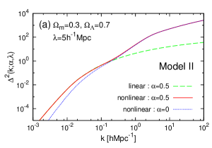
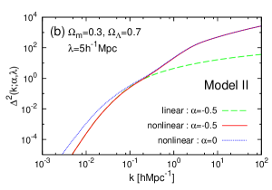
Figure 3: Nonlinear power spectra in Model II; (a) $\alpha=0.5$, (b) $\alpha=-0.5$. We adopt $\Lambda$-CDM and $\lambda=5h^{-1}$Mpc for definiteness. Dashed and solid curves indicate the linear and nonlinear predictions as discussed in the text. For reference, nonlinear Newtonian predictions ($\alpha=0$) are also shown in dotted curves.

In contrast, Model I does not change the nonlinear power spectrum at $z=0$ relative to the $\alpha_{0}=0$ case if one adopts the identical value of $\sigma_{8}$ at $z=0$. Since the linear growth rate for Model I (Eq. (8)) is independent of $k$, the above statement is obvious for linear power spectra. The possible difference would come from the nonlinear evolution. If one evolves $\alpha_{0}=0$ and $\alpha_{0}\not=0$ model spectra from an earlier epoch with the identical amplitude (i.e., $\sigma_{8}$ at that epoch), they lead to different values of $\sigma_{8}$ at $z=0$ because the $\alpha_{0}$-dependent overall growth rate, and thus to different shape of the power spectra due to the nonlinear effect. Instead, if one chooses the identical value of $\sigma_{8}$ at $z=0$, the power spectra of $\alpha_{0}=0$ and $\alpha_{0}\not=0$ models are also identical even taking into account the nonlinear effect. To disentangle Model I from the $\alpha_{0}=0$ model, therefore, one has to compare $\Delta_{\rm NL}^{2}$ at different redshifts. Figure 4 displays the value of $\sigma_{8}$ as a function of $z$. Since this value is computed by extrapolating linear theory, it can be directly obtained from the linear growth rate plotted in Fig. 1. Thus in Model I the structure evolves at a different rate even if the underlying cosmological parameters ($\Omega_{\rm m}$ and $\Omega_{\Lambda}$) are identical. For example, we would need determinations of $\sigma_{8}$ at multiple redshifts to resolve the degeneracy.

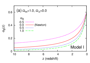
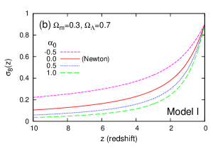
Figure 4: Linearly extrapolated values of $\sigma_{8}(z)$ for different $\alpha_{0}$ in Model I; (a) $\Omega_{\rm m}=1.0$ and $\Omega_{\Lambda}=0.0$, (b) $\Omega_{\rm m}=0.3$ and $\Omega_{\Lambda}=0.7$.

V Comparison with the power spectrum of SDSS galaxies

We are now in a position to explore observational constraints on deviations from Newton’s law of gravity. In order to compare the model predictions described in the previous section against observations, we use the power spectrum of $L_{*}$ galaxies derived from SDSS by Tegmark et al. Tegmark (their Table 3 and http://www.hep.upenn.edu/~max/sdss.html); they compute the power spectrum in the range $0.02h{\rm Mpc}^{-1}<k<0.3h{\rm Mpc}^{-1}$ from a sample of 205,443 galaxies with mean redshift $z\sim 0.1$. Their measurements are in good agreement with our $\Lambda$-CDM model listed in Table I as long as $\alpha=0$.

Figure 5 compares non-linear power spectra for Model II against those for the SDSS galaxies in the $\Lambda$-CDM model; Figure 5(a) shows the $\alpha$-dependence for the $\lambda=10h^{-1}{\rm Mpc}$ case, while Fig. 5(b) illustrates that of varying $\lambda$ for $\alpha=1.0$.

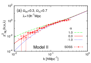
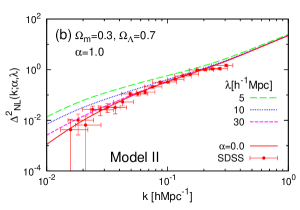
Figure 5: Comparison of power spectra between Model II predictions and the SDSS galaxies (in the $\Lambda$-CDM model); (a) $\alpha=1$ (dotted) and $-1$ (long-dashed) for $\lambda=10h^{-1}$Mpc, and (b) $\lambda=5h^{-1}$Mpc (long-dashed), $10h^{-1}$Mpc (dotted), and $30h^{-1}$Mpc (short-dashed) for $\alpha=1$. For reference, the Newtonian case ($\alpha=0$) is plotted in solid curves. The data points with errors bars represent the results of the SDSS galaxies.

In order to proceed further, we constrain $\alpha$ and $\lambda$ by applying $\Delta\chi^{2}$ statistics press . Model II has two independent parameters ($\alpha$ and $\lambda$), and the overall normalization between the predictions and the data is adjusted by the biasing parameter $b_{*}$ for $L_{*}$ galaxies which we adopt as a third fitting parameter. We then compute the relative confidence levels with respect to the best-fit values assuming that

$$\Delta\chi^{2}(\alpha,\lambda) \equiv \chi^{2}(\alpha,\lambda,b_{*,\text{local~{}min}})$$ (18)

$$-\chi^{2}(\alpha_{\rm min},\lambda_{\rm min},b_{*,\text{min}})$$

follows the $\chi^{2}$distribution for 2 degrees of freedom. In Eq.(18), $\alpha_{\rm min}$, $\lambda_{\rm min}$ and $b_{*,\text{min}}$ denote their best-fit values which globally minimize the value of $\chi^{2}$, while $b_{*,\text{local~{}min}}$ is the value that minimizes the $\chi^{2}$ for a given set of values for $\alpha$ and $\lambda$. The results are summarized in Fig.6; Figure 6(a) plots the contours of $\Delta\chi^{2}(\alpha,\lambda)$; solid, long-dashed and dotted lines indicate the limits at $1\sigma$, $2\sigma$, and $3\sigma$ confidence levels. The amplitude of the power spectrum predicted for Model II is chosen so as to lead to $\sigma_{8}=0.9$ at $z=0$ when $\alpha=0$. Thus using the linear growth rate plotted in Fig. 2, one can compute the contours of $\sigma_{8}$ for Model II in the $\alpha$-$\lambda$ plane which are shown in Fig. 6(b). Figure 6(c) indicates the corresponding $b_{*,\text{local~{}min}}(\alpha,\lambda)$ for the SDSS galaxies with respect to each model. If the linear growth rate were exactly scale-independent and the fit were performed only over the fully linear regime, $\sigma_{8}b_{*,\text{local~{}min}}(\alpha,\lambda)$ plotted in Figs.6(b) and (c) would be constant. In reality, however, the linear growth rate is slightly scale-dependent and the range which we fix, $0.02h{\rm Mpc}^{-1}<k<0.3h{\rm Mpc}^{-1}$, spans a (mildly) nonlinear regime as well. Thus $\sigma_{8}b_{*,\text{local min}}(\alpha,\lambda)$ is not exactly the same over the entire $\alpha$-$\lambda$ plane.

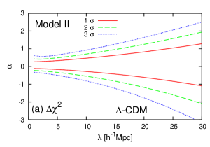
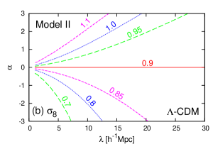
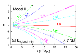
Figure 6: Constraints in the $\alpha$-$\lambda$ plane for Model II in $\Lambda$-CDM cosmology; (a) contours of $\Delta\chi^{2}$, (b) contours of $\sigma_{8}$, (c) contours of $b_{*,\rm local~{}min}$.

VI Conclusion and Discussion

We have used a simple empirical model to parameterize the departure from the Newtonian law of gravity on cosmological scales. We have computed the nonlinear power spectra of density fluctuations predicted in the model assuming a spatially-flat cosmological model and derived the constraints on the amplitude $\alpha$ and the length scale $\lambda$ which characterize the additional Yukawa-type term. Our results are an improvement over the previous attempt by Sealfon et al. as discussed in Secs. I and III. For instance, we obtain the 99.7% confidence limits of $-0.5<\alpha<0.6$ and $-0.8<\alpha<0.9$ for $\lambda=5h^{-1}$Mpc and $10h^{-1}$Mpc, respectively.

Our Model II, Eq. (4), is intended to represent a reasonable approximation to a wide class of possible models which recover Newton’s gravity on small scales but depart from it on large scales. In contrast, Frieman and Gradwohl Frieman91 and Gradwohl and Frieman Gradwohl92 considered a different non-Newtonian gravity model which deviates from Newton’s law on smaller scales, but approaches it asymptotically on larger scales. While their specific model of gravity law is different from that studied here, they extensively discussed the effects on linear perturbation theory and explored the resulting implications for large-scale structure. More recently Nusser, Gubser and Peebles Nusser04 considered cosmological constraints on a similar model of gravity which deviates on small scales. In order to avoid conflict with laboratory tests of Newton’s law, they have to assume that non-Newtonian gravity applies only to dark matter; their model is based on the proposal of Ref. Farrar-Peebles in which the dark sector consists of two mutually coupled fields (dark matter and dark energy), and the length scale $\lambda$ is constant in comoving coordinate. This is why their model substantially changes the nonlinear clustering behavior while our model mostly modifies the weakly nonlinear regime.

In either case, more specific models of non-Newtonian gravity are needed in order to tighten the constraints. Possible proposals include the DGP model in the context of the braneworld scenario Dvali:2000hr ; Deffayet:2000uy , and a relativistic version of the modified Newtonian dynamics Bekenstein04 . These examples are attractive in the sense that they offer specific modified gravity laws on local scales and modified Friedmann equations simultaneously in a consistent fashion. Therefore we could derive more stringent constraints.

Using the SDSS galaxy power spectrum is appropriate for constraining the deviation around $10\sim 100h^{-1}$Mpc scales. If a deviation from Newton’s law occurs at scales below $1h^{-1}$Mpc, strong gravitational nonlinearity will be important, and nonlinear spherical collapse analysis and/or direct N-body simulations would be needed to explore the dynamical consequences for dark halos at galaxy and cluster scales. If the deviation scale is much larger than $100h^{-1}$Mpc, on the other hand, it is unlikely to leave any detectable signature on cosmic structures.

References

- (1) R. A. Knop et al., Astrophys. J. 598, 102 (2003)
- (2) C. L. Bennett et al., Astrophys. J. Suppl. 148, 1 (2003)
- (3) D. N. Spergel et al. Astrophys. J. Suppl. 148, 175 (2003)
- (4) G. R. Dvali, G. Gabadadze and M. Porrati, Phys. Lett. B 485, 208 (2000)
- (5) C. Deffayet, Phys. Lett. B 502, 199 (2001)
- (6) C. Sealfon, L. Verde and R. Jimenez, arXiv:astro-ph/0404111.
- (7) A. Nusser, S. S. Gubser, and P. J. E. Peebles, [arXiv:astro-ph/0412586].
- (8) G. R. Farrar and P. J. E. Peebles, Astrophys. J. 604, 1 (2004)
- (9) E. G. Adelberger, B. R. Heckel and A. E. Nelson, Ann. Rev. Nucl. Part. Sci. 53, 77 (2003)
- (10) C. D. Hoyle, D. J. Kapner, B. R. Heckel, E. G. Adelberger, J. H. Gundlach, U. Schmidt and H. E. Swanson, Phys. Rev. D 70, 042004 (2004)
- (11) C. Deffayet, G. R. Dvali and G. Gabadadze, Phys. Rev. D 65, 044023 (2002)
- (12) A. Lue, R. Scoccimarro and G. D. Starkman, Phys. Rev. D 69, 124015 (2004)
- (13) J. S. Alcaniz and N. Pires, Phys. Rev. D 70, 047303 (2004)
- (14) A. Lue and G. D. Starkman, Phys. Rev. D 70, 101501 (2004)
- (15) N. Arkani-Hamed, H. C. Cheng, M. A. Luty and S. Mukohyama, JHEP 0405, 074 (2004)
- (16) N. Arkani-Hamed, P. Creminelli, S. Mukohyama and M. Zaldarriaga, JCAP 0404, 001 (2004)
- (17) J. A. Peacock and S. J. Dodds, Mon. Not. Roy. Astron. Soc. 280, L19 (1996)
- (18) D. J. Eisenstein and W. Hu, Astrophys. J. 496, 605 (1998)
- (19) M. Tegmark et al. Astrophys. J. 606, 702 (2004)
- (20) W. H. Press, S. A. Teukolsky, W. T. Vetterling, and B. P. Flannery, Numerical Recipes in Fortran (Cambridge University Press, London, 1992), 2nd edition
- (21) J. A. Frieman and B. Gradwohl, Phys. Rev. Lett. 67, 2926 (1991).
- (22) B. Gradwohl and J. A. Frieman, Astrophys. J. 398, 407 (1992)
- (23) J. D. Bekenstein, Phys. Rev. D 70, 083509 (2004).