1. Cosmic Neutrinos for Astrophysicists and Particle Physicists

Both astrophysical and particle-physics questions drive the quest to detect high-energy ($>10^{12}$ eV) cosmic neutrinos. To date, the only two detected neutrino sources, albeit at lower energies ($5-50$ MeV), have illustrated how such observations can significantly impact both fields. First, the observation of the expected flux of neutrinos from the Sun provided astrophysicists with the first direct view of the central engine, not just surface, of the Sun and confirmed the predictions of the standard solar model. For the particle physicists, measurements of the flavor content of this neutrino flux yielded two compelling facts about neutrinos: neutrinos have mass and the weak neutrino eigenstates are not their mass eigenstates. Second, observations of neutrinos emitted from SN1987a in the Large Magellanic Cloud found the predicted prompt neutrino production from the cataclysmic astrophysical event itself, estimated to be of order 99% of the energy release. For particle physicists, the lack of dispersion of the arrival times of these neutrinos over such a long baseline yielded direct limits on the neutrino mass complementary to the contemporary laboratory measurements, and subject to entirely different systematic uncertainties. To date, the observation of every cosmic neutrino source has resulted in a Nobel Prize.

Since neutrino cross sections increase with energy, while backgrounds due to atmospheric neutrino production decrease, most searches for other sources of cosmic neutrinos operate at high energies. Potential sources for these neutrinos include black holes accreting matter in active galactic nuclei (AGN) [1] and in fireballs associated with gamma-ray bursts (GRB). Other considered sources include so-called topological defects (TD) [2], remnants of the early universe which might produce particles with masses comparable to various unification scales such as $10^{25-28}$ eV, that in turn decay to particles producing neutrinos. Observations of AGN and GRB neutrino sources would likely yield insight into astrophysical processes responsible for accelerating the highest energy cosmic rays. Alternatively, observation of TD neutrinos could provide insight into elementary particle physics unobtainable through direct production at terrestrial accelerators.

An additional, well constrained theoretically, source of cosmic neutrinos is produced by the GZK process, the inelastic collision of cosmic ray protons with energies above $10^{19.5}$ eV with the 2.7 K microwave background photons. The collisions occur with a mean free path short compared to cosmological distance scales [3] (of order $4$ Mpc for protons with energy $6\times 10^{20}$ eV). The energy threshold for protons to interact this way, $10^{19.5}$ eV, corresponds to the center-of-mass threshold energy for pion production, about 1200 MeV. The pions’ decay chain produces the so-called GZK neutrinos with energies above $10^{17}$ eV [4], sometimes called the “guaranteed” neutrinos. Assuming our local intensity of such protons is no different than the rest of the universe, the intensity of neutrinos is predicted with only an order-of-magnitude uncertainty [5]. The astrophysical interest in these neutrinos is not that they allow astronomers to look deep into the core of an astrophysical object, but rather that significant deviation from the predicted level would point to a lack of understanding of the relevant energy flows. Note that these predictions are based on proton intensities at $10^{18}$ and $10^{19}$ eV, and do not use measurements at or above the GZK cutoff at $10^{19.5}$ eV. The only significant loophole is that the sources themselves could have an independent internal cutoff at $10^{19.5}$ eV, which would be a cruel coincidence.

The observation of any source of cosmic neutrinos would also provide a unique laboratory for particle physicists. Neutrino interactions above $10^{18}$ eV would probe the electroweak and other interactions at center-of-mass energies beyond those obtainable with modern particle accelerators. Because the standard-model neutrino cross sections are so small, deviations from the standard model due to micro-black hole production or other non-perturbative effects [6] could make them dramatically larger, even by several orders of magnitude. The value of the cross section could be studied by the absorption of neutrinos from a cosmic source through the Earth’s crust and perhaps atmosphere [7]. By contrast, even though cosmic-ray proton or ion interactions probe similarly large center-of-mass energies, their interactions are hadronic, so these additional channels would produce only a small change to their already large cross sections.

2. Quantifying Cosmic Neutrino Detection

In neutrino astronomy, as in other types of astronomy, it is important to distinguish the concepts of flux, intensity, and brightness. I will use these terms as they appear in radiative transfer theory [8], with the modification that I will consider the transfer of number of neutrinos rather than heat. Energy here will refer to the individual energy of each neutrino, $E$, in analogy to the photon frequency, $\nu$, in radiative transfer theory. This convention is consistent with the comprehensive review by Learned and Mannheim [9].

In Table 1, I give the names and units used for the relevant variables. Detectors measure a number of neutrinos, $N_{\nu}$, through an area, $A$, for a given solid angle, $\Delta\Omega$, during a livetime, $\Delta t$, perhaps with some event-by-event energy information. For these proceedings I assume that sources produce a neutrino output that is constant in time; however, based on high energy gamma-ray observations of AGN, observers should be prepared to see flaring objects. For diffuse sources, the relevant variables are intensity, $I$, and brightness, $I_{E}$. Often these are denoted as $d^{3}N/dAd\Omega dt$ and $d^{4}N/dAd\Omega dtdE$, respectively. For point sources, the relevant variables are the flux variables given in the table, which I will not consider further here. Sometimes “intensity” is referred to as “diffuse flux”. Brightness from isotropic models is commonly abbreviated as $dN/dE$, leaving the differentials with respect to area and solid angle as implied, but typically indicated in the units.

The reader should be careful to note the distinction between intensity and brightness. Neutrino intensity is calculated or measured as an integral over energy, so it is not itself a function of energy. The reader will be reminded of the extent of the integral by denoting the intensity as “$I|_{E_{1}}^{E_{2}}$”. In practice, theorists typically provide predictions on neutrino brightness, $I_{E}$, while experimentalists provide sensitivity to neutrino intensities, $I|_{E_{1}}^{E_{2}}$.

For quantifying detection and sensitivities I consider that there exists an unknown brightness of ultra-high energy neutrinos which might depend on $E$, $\theta$, and $\phi$. Assuming the brightness is isotropic, it depends only on $E$. The brightness $I_{E}$ corresponds to no physical observable and for the experimentalist exists only under an integral sign:

$$I|_{E_{1}}^{E_{2}}=\int_{E_{1}}^{E_{2}}I_{E}(E)dE,$$ (1)

where $I|_{E_{1}}^{E_{2}}$ is the number of neutrinos per area per steradian per time with energy between $E_{1}$ and $E_{2}$. (For this reason, brightness may be thought of as an “intensity density”, in analogy with the use of “flux density” for $F_{E}$, but this is not the common term.)

The properties of a neutrino telescope determine the number of events it will detect. First, note that a simple flat particle counter with 100% efficiency is typically described by the area, $A$, and solid angle coverage, $\Delta\Omega$. In general, one only considers the product $\alpha\equiv[A\Delta\Omega]$ vs. energy which usually cannot be uniquely factored (For example, even for a simple flat paddle that is sensitive to particles crossing in either direction, $\alpha=[A\Delta\Omega]$ does not unambiguously factor. It has $\alpha=A\times 2\pi$ not $A\times 4\pi$ due to projection effects. This relative factor of one-half can be absorbed either into an effective area or effective solid angle.) A neutrino telescope typically has a very low efficiency for neutrinos but still can be thought of as having an equivalent area with 100% efficiency, which is typically a strong function of neutrino energy. Thus during a time interval $\Delta t$, a telescope observe $N_{\nu}$ events in the interval $[E_{1},E_{2}]$:

$$N_{\nu}=[\sum_{i=1}^{3}\int_{E_{1}}^{E_{2}}\alpha^{i}(E)\ I_{E}^{i}(E)\ dE]\ \Delta t,$$ (2)

where $i$ is a sum over the three neutrino species. This may be considered the defining equation of $\alpha(E)$ for each neutrino species.

If the number of expected background events is much less than one, one may compare the sensitivities of neutrino telescopes directly using $[A\Delta\Omega](E)\Delta t$. Note that the comparison must be a function of neutrino energy. However, in comparing experiments, one sometimes needs to take into account the expected backgrounds to properly compare the sensitivities. Here I define a quantity [11]

$$\mbox{discovery aperture}=[A\Delta\Omega](E)\Delta t/N_{3\sigma},$$ (3)

where $N_{3\sigma}$ is the number of events the experiment would need to see a $3\sigma$ excess over background. (Note that although high-energy gamma ray detectors often use $5\sigma$ as their standard, they are usually looking for point sources in many places on the sky. Here one is concerned with detection of an isotropic intensity for which there are many times fewer trials.) For a background-free experiment, take $N_{3\sigma}=1$.

Experiments commonly report an effective water-equivalent volume times steradians, $[V^{w.e.}\Delta\Omega]$ rather than $[A\Delta\Omega]$. The variable $[V^{w.e.}\Delta\Omega]$ is defined so that the two descriptions become equivalent in the thin-target approximation via

$$[V^{w.e.}\Delta\Omega](E)\equiv[A\Delta\Omega](E)\times\ell_{int}^{H_{2}O},$$ (4)

where $\ell_{int}^{H_{2}O}$ is the mean interaction length for the neutrino in liquid water at that energy. Specifically, $\ell_{int}^{H_{2}O}=m_{amu}/(\sigma\rho^{H_{2}O})$, where $\rho^{H_{2}O}$ is the density of water, $m_{amu}$ is the atomic mass unit and $\sigma$ is the neutrino cross section per nucleon [12]. In the rare case, typically at very high energies, that the active detector medium itself is large enough to produce some neutrino shielding, it would be less ambiguous to report just $[A\Delta\Omega](E)$.

There are two reasons why the variable $[V^{w.e.}\Delta\Omega]$ is sometimes used. First, the detectors physically occupy volumes; so one can attempt to more sensibly factor this into effective $V^{w.e.}_{eff}$ and $\Delta\Omega_{eff}$. Second, this value does not appear to depend on the neutrino cross section. However, for some high energy telescopes a large portion of their aperture comes from events outside the nominally instrumented volume. Also since neutrino telescopes above $10^{14}$ eV need to include upstream shielding of neutrinos by the Earth, the independence is far from complete. In practice, each telescope may have a very different dependence on the value of neutrino cross section. Since one usually needs the experiments’ own Monte Carlo simulations to know the variance of the sensitivity with cross section, neutrino telescope collaborations would do better to publish either $[A\Delta\Omega](E)$ or $[V^{w.e}\Delta\Omega](E)$ for values of 75%, 100% and 125% of the nominal cross sections used.

Looking at the typical neutrino brightness predictions [1], [2], [5] in the context of equations 2 and 4, it becomes apparent that for neutrino energies $10^{13}$ eV to $10^{15}$ eV, one needs detectors with $[V^{w.e.}\Delta\Omega]$ of order $1-10$ km³-sr. Already these sizes demand instrumenting large natural volumes since they are larger than anything that can be reasonably manufactured. Several telescopes are currently running or under construction that employ optical techniques in the clearest media known: Antarctic ice (Amanda, IceCube) and deep water (Baikal, Antares, Nestor, and Nemo). The limiting size of such detectors is determined by the effective attenuation length of light (including scattering), 50-100 m in these media. This length determines spacing and the practicality of deployment, yielding detectors that may achieve apertures up to $10$ km³-sr.

For energies above $10^{18}$ eV, one can attempt to detect the GZK neutrinos whose brightness is fairly well understood. The desired size increases to at least 1,000 km³-sr. So while the standard optical detection techniques are well suited to energies up to $10^{15}$ eV, larger volumes are needed at higher energies. As will be described in Sections 3 and 4, neutrino-induced showers also produce radio emission up to tens of GHz and acoustic emission to hundreds of kHz. Since in some materials the attenuation length for these emissions may exceed a kilometer, several groups are exploiting these techniques to achieve the extremely large apertures. (Additional information may also be found in another recent review [13].) Two other techniques also offer the possibility of such larger apertures: atmospheric observations from space and exploiting mountain ranges and the finite lifetime of the $\tau$ lepton; these will be discussed in Section 5. Based on some lessons learned from this exercise, I present a proposal on reporting results in Section 6.

3. Radio Detection

When a neutrino interacts in material, it produces a shower of relativistic particles. For energies above $10^{15}$ eV, about 20% of the neutrino energy appears as a relativistic hadronic shower through the “inelasticity” of the neutrino interaction with matter. The hadronic shower eventually becomes electromagnetic (electrons, positrons, and photons) through production of $\pi^{0}$ mesons which quickly decay to photons. For charged-current interactions, which are 70% of the interactions at these energies, a charged lepton, $e$, $\mu$, or $\tau$ is also produced with the remaining energy, each of which eventually deposits some electromagnetic energy as well. These particles are typically moving faster than the speed of light in the material, $c/n_{refr}$, and produce the optical Cherenkov radiation that is the basis for many neutrino telescopes.

In the early 1960’s, Gurgen Askaryan realized [14] that a strong radio component (up to $\sim$ 10 GHz, lasting of order 1 ns) of Cherenkov emission would be produced as well. For interactions in matter, a $(10-30)$% charge excess of electrons over positrons will develop since the target material contains electrons at rest and no positrons. For wavelengths longer than the lateral size of the shower (a few centimeters in radius) the emission becomes coherent. Unlike the optical radiation, which is incoherent, the power of radio emission grows as the square of the energy of the shower. At $10^{18}$ eV, about $10^{8}$ electrons radiate in phase, producing a large electromagnetic pulse (of order $500$ V/m at 1 m.) Askaryan’s calculations were subsequently confirmed by independent groups using modern shower simulations based on EGS [15] and with GEANT [16], which are now in basic agreement. The predicted characteristics and intensity of emission were further demonstrated in a series of experiments at SLAC [17]. The square-law dependence of the power in incident neutrino energy, which helps for high neutrino energies, unfortunately also implies a relatively high threshold due to the presence of irreducible thermal noise in any detection medium. Thresholds as low as $10^{17}$ eV are achieved with this technique, perhaps extendible as low as $10^{16}$ eV. In his original work, Askaryan presciently pointed out that detectors could be based on large ice sheets, natural salt formations and the lunar surface material which to date still form the basis of this technique.

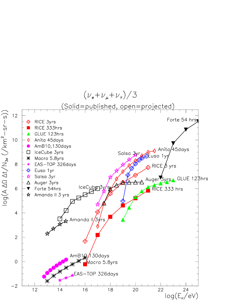
Figure 1: My attempt to convert several telescopes’ sensitivity to a common discovery aperture, $[A\Delta\Omega]\Delta t/N_{3\sigma}$, as defined in the text. The quantity presented here is the average over all three neutrinos species, for illustrative purposes but an analysis breaking it down by flavor, such as in Ref. [40], may also be done. The values presented here should be taken as representative, awaiting official numbers from the collaborations themselves, so comparisons should be taken to within a $\log_{10}(2)=0.3$ “grain-of-salt” on the vertical and horizontal scales. Current results are presented with solid symbols, projected results are with open symbols. Note that some projected telescopes are funded and under construction, while others are in the conceptual stage. Times are live time. CAVEAT: Because this plot presents the average over three neutrino flavors, telescopes that obtain most of their sensitivity from one flavor (Amanda, Auger) would do better relative to other experiments in pure-flavor plots. When space allows, three separate plots for the individual flavors would be better.

The RICE [18] telescope consists of 20 dipole antennas sensitive after filtering from 200 to 500 MHz placed on the same strings as the Amanda neutrino telescope at the South Pole. The array comprises a $200\times 200\times 200$ m array. The ice on the Antarctic plateau has exceptionally long attenuation lengths, in excess of 1000 m, as extracted from airborne ground-penetrating radar and surface measurements in Greenland, Iceland, laboratory measurements and a new South Pole measurement [19]. Hence, the sensitive volume is much larger than the array itself, achieving above 10 km³-sr above $10^{18}$ eV with nearly full-time duty cycle. RICE has placed limits on cosmic neutrinos with energies above $10^{16}$ eV based on a 3-year dataset and data taking is ongoing. The RICE aperture is compared to current and expected techniques in Figure 1 and Table 2. Studies of an extension of this technique, X-RICE [20], to holes spread over an area up to 10⁴ km² in Antarctica could be sensitive to tens to hundreds of GZK neutrinos per year.

Based on an idea of Zheleznyk and Dagkesamanskii [21], the emission from neutrino interactions in the outer $10-20$ m of the Moon’s surface is detectable above its thermal black-body emission for energies above $10^{20}$ eV by terrestrial radio telescopes. A 12-hour search using the Parkes 64 m dish in Australia [22] did not see any events but had significant radio-frequency interference. A search using radio telescopes at the Goldstone tracking station (GLUE) [23] used two antennas in coincidence to eliminate terrestrial background. GLUE did not see any events after 123 hours of observations with a threshold of $10^{20}$ eV and achieving $[V^{w.e.}\Delta\Omega]$ of order 500 km³-sr, although unlike RICE, the duty cycle due to available telescope time corresponded to only $5\times 10^{-3}$. The GLUE aperture is compared to current and expected techniques in Figure 1 and Table 2. Future attempts using this technique are underway at the Kalyazin radiotelescope [24].

The FORTE experiment [25] used a space-based platform with a log-periodic antenna array designed for VHF lightning observations to achieve a total of 2.3 days integrated observation of Greenland ice. (Its orbit did not provide a view of Antarctic ice.) Since the radio emission travels through the ionosphere, there is a characteristic frequency-dependent delay which allowed suppression of backgrounds. Because FORTE operated at a lower frequency and bandwidth than other experiments (22 MHz BW from 30 to 300 MHz) it suffered from a higher threshold, $10^{22}$ eV. However at these frequencies the Cherenkov radio emission diffracts due to the finite length of the shower and thereby fills a large solid angle. FORTE thereby achieves an impressive $[V^{w.e.}\Delta\Omega]\sim 100,000$ km³-sr. Its duty cycle was $\sim 3\times 10^{-3}$. The FORTE aperture is compared to current and expected techniques in Figure 1.

The ANITA [26] detector combines many of the most attractive features of the above experiments into one project designed to be sensitive to the GZK neutrinos. ANITA will be a balloon-borne payload of dual-ridged gain horn antennas (200-1200 MHz after filtering) flying for a total of 60 days beginning in the 2006-07 season. At an altitude of 37 km above the Antarctic ice, ANITA will have a threshold of approximately $10^{17}$ eV and with an instantaneous view of 1.5 million km³ of ice, yielding an aperture of $\sim$20,000 km³-sr. Assuming an 18-day flight per year, the duty cycle is an annualized 0.05. A test flight in the 2003-04 season, ANITA-lite [26], indicated a sufficiently radio-quiet environment and successfully demonstrated the essential in-flight systems. This engineering flight worked well enough that a new limit may be extracted from these data. The ANITA aperture is compared to other expected results in Figure 1 and Table 2.

A complementary approach that is still in the conceptual stage is to instrument large natural salt formations with antennas much in the style of the RICE detector. Salt domes which are large and dry offer attenuation lengths in excess of a few hundred meters which, accounting for the increased density, correspond to nearly a kilometer water-equivalent attenuation length. Example detectors include the SND [27], SALSA [28] and ZESANA [29] concepts which could instrument many tens of cubic kilometers of salt. Because the antennas are closer to the events than ANITA, the threshold could be an order-of-magnitude lower. Even though $[V^{w.e.}\Delta\Omega]$ is comparable or even lower than ANITA, because the duty cycle is much larger, the ultimate sensitivity of salt-based detectors is the largest of any considered and has the lowest threshold. In addition, there would be closer to full-sky coverage and a larger duty cycle for flaring sources. Because salt-domes are generally covered by an overburden of rock, they are naturally shielded from man-made electromagnetic sources on or above the Earth’s surface. The SALSA aperture is compared to other expected results in Figure 1 and Table 2.

4. Acoustic Detection

In addition to the radio detection idea, Askaryan described how ultra-high energy neutrino interactions could be detected by underwater acoustic techniques [30]. A $10^{21}$ eV neutrino shower under water deposits 150 J of heat through ionization in a highly localized region. As a result, a hydrothermal pressure impulse lasting of order 10 $\mu$s propagates outward as a thin pancake. Verification of the production of this pulse was performed at accelerators at Brookhaven, Uppsala, and ITEP [31].

Noise sources in the ocean include turbulence, surface waves, wind, oceanic traffic, precipitation, biological systems and thermal noise. The noise spectral density goes through a minimum in the 10 kHz range which is also where the power spectral density of the neutrino-induced pressure pulse would peak. Work is underway to characterize the noise environment in solids such as Antarctic ice and salt domes.

Over the years, several detectors have been proposed, generally using hydrophone arrays in the deep ocean. Considerable interest has been renewed lately. R&D for acoustic sensors and site selection was discussed recently at a workshop dedicated to the acoustic technique [32] and can be found among the slides. Hydrophone arrays near Kamchatka (SADCO) [33], Rona (U.K.) [34], and TREMAIL near the Antares site have been used for preliminary environmental measurements and testing of reconstruction techniques. At the acoustic workshop, a large number of groups showed significant and broad progress in development of hydrophones and pre-amplifiers for the Nemo, Antares, and Lake Baikal sites. The existing Lake Baikal sensors may even show a hint of excess consistent with an acoustical neutrino signal [35] and their data-taking continues. Detector development for solid media such as Antarctic ice and salt domes is also underway [36]. Well-understood calibrators for solid and liquid acoustic detectors are critical; methods under development include submerged implosions and noise from airplanes. Until recently, sensitivity estimates have been largely analytic, but Monte Carlo simulation tools for acoustic detection are being developed [37] that will aid future design and sensitivity estimates.

Here I discuss one acoustic-based telescope in detail, the SAUND detector [38], since it has been carried through to completion, including a publication. Located in the deep sea off of the Bahamas, the SAUND collaboration instrumented 7 hydrophones arranged in a star pattern using a subset of the U.S. Navy’s AUTEC array in the Bahamas to detect the impulse in frequency bands $7-50$ kHz. The hydrophones are deep (1.6 km) and sheltered by several islands and shoals with little shipping traffic. The observed noise floor, consistent with $\nu^{-1.7}$ Knudsen noise set the threshold at $\sim 10^{21}$ eV but could be reduced by finding or building a hydrophone array with closer spacing. Imploding light bulbs at various distances and depths tested the event reconstruction and were consistent with attenuation lengths of 500 to 1000 m. Refraction effects become significant at 1000 m and beyond. The collaboration ran a physics run for 195 days. Although the $[V^{w.e.}\Delta\Omega]$ of about 100 km³-sr is still too small for these energies, it should be noted that SAUND’s geometry was not optimal for the pancake-like shape of the acoustic pulse. There is hope that arrays with optimized geometry and also solids such as large salt domes could provide one or two orders of magnitude more aperture through larger signal and lower backgrounds. The SAUND group is preparing to install SAUND-2 to instrument 1500 km³ of sea water [39].

A hybrid detector combining both radio and acoustic techniques holds some promise. Due to the extreme difference in the velocities of propagation of radio versus sound waves, and their different polarization properties, a simultaneous detection of the same event using the two techniques might yield interesting information. However, if the thresholds and sizes of the two arrays are significantly different, they would be unlikely to make any simultaneous observations.

Considerable new activity has begun in the last couple of years in the field of acoustic detection techniques for neutrino astronomy after a relatively quiet two decades. The radio and acoustic fields are now so rich that future summaries ought to be divided among two speakers to do the fields justice.

5. Other neutrino telescope techniques

We wish to compare the radio and acoustic techniques to other neutrino telescopes that have run or will turn on that are sensitive to neutrinos above $10^{12}$ eV. Often it is difficult based on the published materials to convert the reported limits into the sensitivity curve (discovery aperture) $[A\Delta\Omega]\Delta t/N_{3\sigma}$ versus energy. I have converted their limits in a hopefully reasonable way [40] and show the comparisons in Figure 1. Numbers of expected events based on these estimates and equation 2 are shown in Table 2.

In the $10^{12}$ to $10^{15}$ eV regime, several detectors have looked for muons produced by $\nu_{\mu}$ charged-current neutrino interactions or pion decay in the material below them. MACRO was a small detector but ran for nearly 6 live years and set limits on the neutrino intensity between $10^{13}$ and $10^{16}$ eV. Recently Amanda-B10, which is a much larger detector, set a stronger limit on the $\nu_{\mu}$ intensity between $5\times 10^{13}$ and $5\times 10^{14}$ eV in less time. The Lake Baikal neutrino telescope [41] reports limits with a threshold around $10^{13}$ eV for $\nu_{\mu}$ interactions. Using a different technique EAS-TOP [42] ran for 326 days and reported limits for $E$ between $10^{14}$ and $10^{15}$ eV based on the rate of horizontal extensive air showers. The Amanda-II detector [43], consisting of 19 strings will set even strong bounds. As shown in the figure, from $10^{14}$ to $10^{17}$ eV the IceCube [44] detector will greatly increase the current sensitivity. Telescopes based in the Mediterranean (Antares, Nemo and Nestor)  [45], using sea water rather than Antarctic ice will both overlap and extend the sky coverage of IceCube. The sensitivities of a few representative optical-based telescopes are compared with the radio and acoustic techniques in Figure 1.

Above about $10^{16}$ eV, a few other techniques besides radio and acoustic offer the possibility of extending beyond 10 km³-sr. The Auger collaboration would be sensitive to $\nu_{\tau}$ interactions in nearby mountains; because due to the finite lifetime of the $\tau$ lepton, they would be able to detect its decay with $[V^{w.e.}\Delta\Omega]$ as large as 10 km³-sr above $10^{18}$ eV. This has the advantage that it can be done parasitically with an existing experiment. The EUSO collaboration [46] showed how observing large volumes of the atmosphere from an orbiting platform could be sensitive to $[V^{w.e.}\Delta\Omega]$ of order 100 km³-sr with a high duty cycle, subject to the detector being launched. Still, as shown in the figure, the apertures achievable with radio detection are larger. Radio-based detectors in embedded in salt or ice, with their relatively low threshold, large duty cycle and large sky coverage may eventually be the most versatile ultra-high energy radio-based neutrino detector.

6. Proposal for how neutrino telescopes should report results

Because I do not have access to each collaboration’s internal Monte Carlo simulations and/or calculations I took some liberties of interpretation in converting the reported numbers into a common framework. The most common problem was that some limits already included the neutrino cross section and even particular models for neutrino brightness that were hard to untangle. Sometimes “effective area” or “effective volume” was quoted without stating for which solid angle it was defined. Sometimes the “effective volume” did not state if it was for water-equivalent or for the actual medium’s density. Sometimes it was not even clear if deadtimes were already included in the reported livetime or absorbed into the limit as an efficiency. As a result of this effort, I propose here how neutrino telescopes should report their sensitivity in the future so that telescopes can be meaningfully compared. Another advantage of following this proposal is that if a new model arrives long after the collaboration is still able and willing to run its simulation tools, meaningful limits can still be extracted via Equation 2. (Dramatically different interaction models, for example changing neutrino cross sections by orders of magnitude, would still require separate study.)

• Quote $[A\Delta\Omega]$ and/or $[V^{w.e}\Delta\Omega]$ as a function of energy for each neutrino species, which I will call here the aperture. Note that this includes upstream attenuation of neutrinos by the Earth.

• Specify which cross sections were used.

• Specify the livetime $\Delta t$ the observations correspond to. Deadtime corrections belong here, not in the quoted aperture.

• Give the expected background events during the livetime $\Delta t$, if any. If this depends on the threshold applied, these steps should be repeated for a few thresholds.

• Quote the aperture for cross sections 75% and 125% the nominal value used. If the effect is non-linear, more variations would be appropriate.

• Quote the aperture for some variation of the inelasticity, $y$, as well.

• Number of events observed, if any. If significant, this list should be repeated for a range of detector thresholds and observed events.

With the above information, comparisons could be directly made without subsequent interpretation. Also limits on new models could be set using old data.

7. Conclusions

Detection of cosmic neutrinos offers a fertile ground for addressing interesting questions in astrophysics as well as elementary particle physics. The generation of neutrino telescopes coming online within the next 3–5 years will greatly increase the existing apertures and probe theoretically interesting regions. Below $10^{16}$ eV, neutrino astronomy is the domain of the optical Cherenkov detectors. Above $10^{17}$ eV, radio-based detectors offer the largest apertures and are well matched to the expected spectrum of GZK neutrinos. The acoustic technique also shows promise if ongoing work to demonstrate lower energy thresholds is successful. The variety of techniques applied to the challenge of neutrino astronomy is impressive. I have presented a proposal for describing the sensitivity of these widely varying techniques in a common framework.

Acknowledgments

The author thanks the Nobel Symposium Committee for its hospitality and organization of an excellent workshop. This work was partially supported by the U.S. Department of Energy’s Office of Science and the National Aeronautics and Space Administration. I thank the many representatives of the collaborations mentioned here as well as Amy Connolly, Bob Cousins, and Jay Hauser for helpful discussions.

term	symbol	with arguments	units for neutrinos
neutrinos	$N_{\nu}$	$N_{\nu}$	(unitless)
neutrino intensity	$I$	$I(\theta,\phi)$	[length]-2 [sr]-1 [time]-1
neutrino brightness, or	$I_{E}$,	$I_{E}(E,\theta,\phi)$	[length]-2 [sr]-1 [time]-1 [energy]-1
neutrino specific intensity
net flux	$F_{E}$	$F_{E}(E)$	[length]-2 [time]-1 [energy]-1
flux density
total integrated flux,	$F$	$F$	[length]-2 [time]-1
or surface flux
or flux density

Table 1: Definitions of relevant quantities used here. Note that the term “flux density” finds more than one use in the literature, but the more common is for $F_{E}$.

		$N_{\mbox{events}}$
		Top. Def.	GZK		WB
Telescope	Duration	(PS)	(min)	(max)
Amanda-II	3 live years	0.6	0.02	0.1	125
ANITA	45 live days	44	4.8	18	6.5
Auger	3 live years	0.7	1.0	3.0	1.1
EUSO	2.7 live years	18	0.9	3.6	1.9
IceCube	3 live years	1.1	0.5	1.3	281
RICE	3 live years	3.3	0.9	2.8	1.2
SALSA-1000 Rx	3 live years	50	58	194	56

Table 2: Estimated number of events from various models that would be observed in some characteristic telescopes which are being constructed or considered. The WB model is a $E^{-2}$ spectrum with the Waxman-Bahcall [47] coefficient. Disclaimer: these numbers include my own estimates of the detector apertures as described in the text. A more accurate comparison could be achieved if more of the experiments follow the proposal described in the text. Here the Amanda numbers correspond to $\nu_{\mu}$ only; they have also recently reported sensitivity to other flavors.

References

- [1] Mannheim, K., Protheroe, R., Rachen, J., Phys Rev. D 63, 023003 (2001).
- [2] Yoshida, S. et al., Phys. Rev. Lett. 81, 5505 (1998); Protheroe, R. and Stanev, T., Phys. Rev. Lett. 77 3708 (1996).
- [3] Greisen, K., Phys. Rev. Lett. 16, 748 (1966); Zatsepin, G. and Kuzmin, V., JETP Lett. 4, 78 (1966).
- [4] Berezinsky, V. and Zatsepin, G., Phys. Lett. B 28, 423 (1969); Sov. J. Nucl. Phys. 11, 111 (1970).
- [5] The estimates quoted here are from Engel, R., Seckel, D. and Stanev, T., Phys. Rev. D 64, 093010 (2001). See references therein for other calculations.
- [6] See one compilation in Han, T. and Hooper, D. New J. Phys. 6, 150 (2004). See also Alvarez-Muniz, J. et al., Phys. Rev. D 65, 124015 (2002); Fiore, R. et al., Phys. Rev. D 68, 093010 (2003).
- [7] Kusenko, A. and Weiler, T., Phys. Rev. Lett. 88, 161101 (2002); Alvarez-Muniz, J. et al. Phys. Rev. Lett. 88, 021301 (2002).
- [8] Rybicki, G. and Lightman, A., Radiative Processes in Astrophysics, Wiley-Interscience, 1979.
- [9] Learned, J. and Mannheim, K., Ann. Rev. Nucl. Part. Sci., 50 679 (2000).
- [10] Williams, D., Ph.D. Dissertation, University of California Los Angeles, 2004.
- [11] Note that the parameter here is divided by what Super-K calls a “green’s function” in their fluence analysis, but adapted here to a diffuse intensity case: Fukuda, F. et al. (Super-K collaboration), Ap. J. 578, 317 (2002).
- [12] The most common values of cross section used are Gandhi, R. et al., Phys. Rev. D. 58, 093009 (1998).
- [13] Nahnhauer, R., Proc. XXI Conf. on Neutrino Physics and Astrophysics, astro-ph/0411715 (2004).
- [14] Askaryan, G., Soviet Physics JETP 14, 441 (1962); Askaryan, G., Soviet Physics JETP 21, 658 (1965).
- [15] Zas, E., Halzen, F. and Stanev, T., Phys. Rev. D 45, 362 (1992); Alvarez-Muniz, J. and Zas, E., Phys. Lett. B 434 396 (1998) and references therein.
- [16] Frichter, G., Ralston, J. and McKay, D., Phys. Rev. D 53, 1684 (1996); Razzaque, S. et al., in Proc. RADHEP-2000, AIP#579 (2001).
- [17] Saltzberg, D., Gorham, P., Walz, D. al., Phys. Rev. Lett. 86, 2802 (2001); Gorham, P. et al., astro-ph/0412128 (2004).
- [18] Kravchenko, I. et al., Astropart. Phys. 19, 15 (2001); Kravchenko, I. et al. Astropart. Phys. 20, 195 (2003); RICE=Radio in Ice Cherenkov Experiment.
- [19] For example, Bogorodsky, V. and Gavrilo, V., “Ice: Physical Properties,” (Modern Methods of Glaciology, Leningrad, 1980); Bogorodsky, V., Bentley, C. and Gundmandsen, P., “Radioglaciology,” (Reidel Publishing, Dordrecht, 1985). A comprehensive list of sources is available in the second entry of Ref. [18]. A direct measurement at the South Pole was recently completed, see Barwick, S. et al., J. Glac., in press with preprint at http://www.lns.cornell.edu/~dzb/tem/RF-eps-im.pdf.
- [20] Seckel, D. and Frichter, G., Proc. 26th ICRC, AIP#516 (1999); Seckel, D. in Proc. RADHEP-2000, AIP#579 (2001).
- [21] Zheleznykh, I., Proc. Neutrino 88, 528 (1988); Dagkesamanskii, R. and Zheleznykh, I., Soviet Physics JETP 50, 233 (1989).
- [22] Hankins, T., Ekers, R. and O’Sullivan, J., MNRAS 283, 1027 (1996).
- [23] Gorham, P. et al., Phys. Rev. Lett. 93, 041101 (2004); GLUE=Goldstone Lunar Ultra-high energy neutrino Experiment.
- [24] Zheleznykh, I. and Dagkesamanskii, R., private communication (2004). See also Beresnyak, A. astro-ph/0310295.
- [25] Lehtinen, N. et al., Phys. Rev. D 69, 013008 (2004); FORTE=Fast On-orbit Recording of Transient Events.
- [26] Silvestri, A., Proc. Int’l School of Cosmic Ray Astrophysics, astro-ph/0411007 (2004); ANITA=ANtarctic Impulsive Transient Antenna.
- [27] Chiba, M. et al. in Proc. RADHEP-2000, AIP#579; An updated manuscript is in preparation, Chiba, M. private communication (2004); SND=Salt Neutrino Detector.
- [28] Gorham, P. et al., Nucl. Instr. and Meth A490, 476 (2002); Saltzberg, D. in Proc. SPIE vol 4858 p. 191 (2003); Williams, D. and Connolly, A. in D. Williams UCLA Ph.D dissertation, chapter 5 (2004); Gorham, P. et al. astro-ph/0412128 (2004); SALSA=SALt dome Shower Array.
- [29] van den Berg, A. et al. in KVI Annual Report (2004); van den Berg, A. in Symposium on “Core Business: heat production of the Earth” (2004); ZESANA=ZEchstein SAlt Neutrino Array.
- [30] Askaryan, G., Sov. J. Atom. Energy 3, 921 (1957); Askaryan, G. and Dolgoshein, B., JETP Lett. 25, 213 (1977). For a more complete history see John Learned’s slides in Ref. [32] and from RADHEP-2000.
- [31] Sulak, L. et al., Nucl. Instr. and Meth. 161, 203 (1979); See Nahnhauer, R. and Rostovstev, A. talks in Ref. [32]. Albul, V. et al., Instrum. Exp. Tech. 44, 327 (2001).
- [32] See http://hep.stanford.edu/neutrino/SAUND/workshop/ and links therein; SAUND=Study of Acoustic Ultra-high energy Neutrino Detection.
- [33] Dedenko, L. et al. in Proc. RADHEP-2000 (2001); See Zheleznykh, I. talk in Ref. [32]; SADCO=Sea Acoustic Detection of Cosmic Objects.
- [34] See talks by Rhodes, C., Thompson, L., and Waters, D. in Ref. [32].
- [35] Budnev, N. et al. in manuscript presented at Ref. [32].
- [36] See talks by Nahnhauer, R. and Fink, M. in Ref. [32].
- [37] See talks by Waters, D. and Niess, V. in Ref. [32].
- [38] Vandenbrouke, J., Gratta, G. and Lehtinen, N., to appear in Astrophysics Journal, astro-ph/0406105; Lehtinen, N. et al. Astropart. Phys. 17, 279 (2002).
- [39] Gratta, G., private communication (2005).
- [40] Details of the calculation can be found at http://www.physics.ucla.edu/~saltzbrg/uhenu.ps (2003).
- [41] Spiering, C., these proceedings; Spiering, C. in Proc VLVT Workshop, astro-ph/0404096.
- [42] Aglietta, M. et al. Phys. Lett. B 333, 555 (1994).
- [43] Barwick, S., Proc. 27th ICRC (2001); http://area51.berkeley.edu/manuscripts/20010601xx-ICRC_AmIIv3.pdf
- [44] Karle, A. et al., astro-ph/0209556 (2002).
- [45] Sokalski, I. et al. (Antares Collab.) hep-ex/0501003; Tsirigotis, A. et al. (Nestor Collab) Eur. Phys. J. C33 S956 (2004); Migneco, E. et al. (Nemo Collab.), Proc. VLVT Workshop, 5. (2004).
- [46] Bottai, S. and Giurgola, S. Proc. 28th ICRC, 1113 (2003); EUSO=Extreme Universe Space Observatory.
- [47] Waxman, E. and Bahcall, J., Phys. Rev. D59 023002 (1999); Waxman, E. and Bahcall, J., Phys. Rev. D64 023002 (2001).