Uncorrelated Measurements of the Cosmic Expansion History and Dark Energy from Supernovae

Abstract

We present a method for measuring the cosmic expansion history $H(z)$ in uncorrelated redshift bins, and apply it to current and simulated type Ia supernova data assuming spatial flatness. If the matter density parameter $\Omega_{m}$ can be accurately measured from other data, then the dark energy density history $X(z)=\rho_{X}(z)/\rho_{X}(0)$ can trivially be derived from this expansion history $H(z)$. In contrast to customary “black box” parameter fitting, our method is transparent and easy to interpret: the measurement of $H(z)^{-1}$ in a redshift bin is simply a linear combination of the measured comoving distances for supernovae in that bin, making it obvious how systematic errors propagate from input to output.

We find the Riess et al. (2004) “gold” sample to be consistent with the “vanilla” concordance model where the dark energy is a cosmological constant. We compare two mission concepts for the NASA/DOE Joint Dark Energy Mission (JDEM), the Joint Efficient Dark-energy Investigation (JEDI), and the Supernova Accelaration Probe (SNAP), using simulated data including the effect of weak lensing (based on numerical simulations) and a systematic bias from K-corrections. Estimating $H(z)$ in seven uncorrelated redshift bins, we find that both provide dramatic improvements over current data: JEDI can measure $H(z)$ to about 10% accuracy and SNAP to 30-40% accuracy.

I Introduction

Observational data on type Ia supernovae (SNe Ia) indicate that the expansion of our universe is accelerating (Riess et al., 1998; Perlmutter et al., 1999). This can be explained by the presence of dark energy. Various dark energy models have been considered, e.g.  scalar fields (Freese et al., 1987; Linde, 1987; Peebles & Ratra, 1988; Wetterich, 1988; Frieman et al., 1995; Caldwell, Dave & Steinhardt, 1998) and modified gravity (Sahni & Habib, 1998; Parker & Raval, 1999; Boisseau et al., 2000; Deffayet, 2001; Mersini, Bastero-Gil, & Kanti, 2001; Freese & Lewis, 2002; Carroll et al., 2004) — see Padmanabhan (2003) and Peebles & Ratra (2003) for recent reviews.

Although current data seem consistent with a cosmological constant (e.g., Choudhury & Padmanabhan (2004); Chen & Ratra (2004); Daly03 ; Daly & Djorgovski (2004); Dicus & Repko (2004); Hannestad & Mortsell (2004); Simon, Verde, & Jimenez (2004); Wang & Tegmark (2004); Jassal, Bagla, & Padmanabhan (2005)), the uncertainties are large and more exotic models are not ruled out (e.g., Alam, Sahni, & Starobinsky (2004); Capozziello, Cardone, & Francaviglia (2004); Huterer & Cooray (2004); Feng et al. (2004); Wang et al. (2004a)). To uncover the nature of dark energy, and differentiate among various dark energy models, it is important that we extract dark energy constraints in a model-independent manner (Wang & Garnavich, 2001; Wang & Lovelace, 2001; Wang & Freese, 2004). The perils of model assumptions and simplified parametrization of dark energy have been shown in Maor, Brustein, & Steinhardt (2002); Wang & Tegmark (2004); Bassett, Corasaniti, & Kunz (2004).

Throughout this paper, we assume spatial flatness as motivated by inflation. Calibrated cosmological standard candles such as SNe Ia measure the luminosity distance $d_{L}(z)=(1+z)r(z)$, where the comoving distance

$$r(z)=\int_{0}^{z}\frac{dz^{\prime}}{H(z^{\prime})}=H_{*}^{-1}\int_{0}^{z}\frac{dz^{\prime}}{h(z^{\prime})}$$ (1)

where $c=1$, $H_{*}=100$km s^-1Mpc^-1 and

$$h(z)\equiv H(z)/H_{*}=h(0)\left[\Omega_{m}(1+z)^{3}+\Omega_{X}X(z)\right]^{1/2},$$ (2)

with $X(z)\equiv\rho_{X}(z)/\rho_{X}(0)$ denoting the dark energy density function. Determining if and (if so) how the dark energy density $X(z)$ depends on cosmic time is the main observational goal in the current quest to illuminate the nature of dark energy. Given a precise measurement of the matter density fraction $\Omega_{m}$ (from galaxy redshift surveys, for example), the dark energy density function $X(z)$ can be trivially determined from $H(z)$ via equation (2).

Numerous methods for this have been developed and applied in the recent literature, either by parametrizing $X(z)$ in terms of an equation of state and perhaps additional parameters or by aiming for more model-independent constraints (e.g., Wang & Tegmark (2004)). Equation (1) shows that the data directly constrain the cosmic expansion history $H(z)$ — in principle. The information-theoretically minimal error bars on $H(z)$ that can be obtained from supernovae were derived in Tegmark (2002) using a Fisher matrix approach. Yet no optimal method for doing this in practice has been found other than the “black box” approach of parametrizing $H(z)$ somehow and fitting to the data. Ideally one would like to measure $H(z)$ in many redshift bins with uncorrelated error bars, but Tegmark (2002) found that parametrized fits tend to yield broad and difficult-to-interpret window functions, i.e., the measurement in a given redshift bin depended also on supernova data far outside that redshift range. Huterer & Cooray (2004) strengthened this conclusion by showing that uncorrelated measurements of the expansion history (computed by diagonalizing the Fisher matrix) tended to probe a broad redshift range. The approach most similar to ours is that of Tegmark (2002); Daly03 ; Daly & Djorgovski (2004), where $H(z)^{-1}$ is measured by numerically differentiating equation (1). These papers tackle the challenge of differentiating sparse and noisy data by performing a polynomial fit for $r(z)$: Tegmark (2002) performs a global fit whereas Daly03 ; Daly & Djorgovski (2004) improve this with a local fit within a sliding window.

The purpose of the present paper is to solve this problem optimally, presenting a method giving uncorrelated measurements of the expansion history in arbitrary redshift bins. We will see that this method is both easy to implement and easy to interpret. We describe our method in Sec.2. We present our results in Sec.3 and discuss our conclusions in Sec.4.

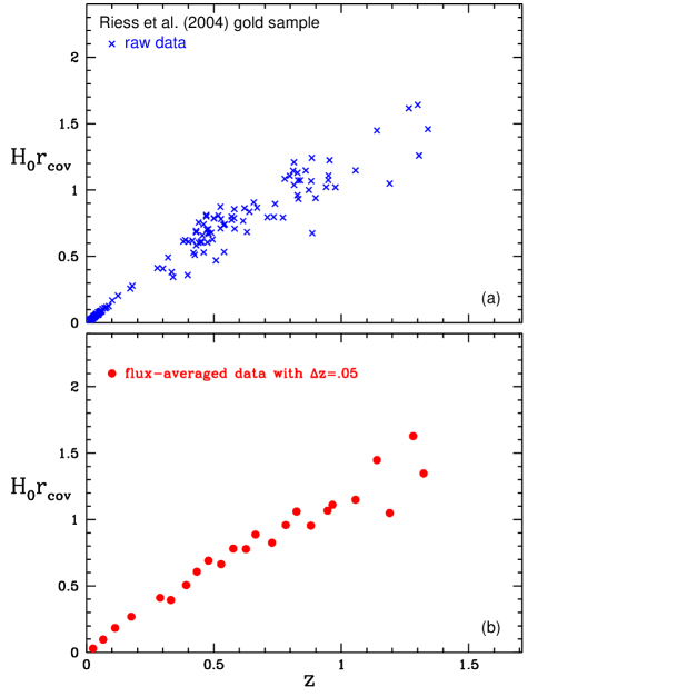
Figure 1: Data used. The measured dimensionless comoving distances are shown for the Riess et al. (2004) “gold” sample before (top panel) and after (bottom panel) flux averaging. The cosmic expansion $h(z)$ is simply the inverse of the derivative of this, so the visually obvious fact that the derivative is falling immediately tells us that the universe was denser and faster expanding in the past.

II Method

Assuming that the redshifts of SNe Ia are accurately measured, we can neglect redshift uncertainties, and simply treat the measured comoving distances $r(z_{i})$ to the supernovae (plotted in Figure 1) as the observables. In terms of $\mu_{0}$, the distance modulus of SNe Ia, we have

$$\frac{r(z)}{\mbox{1 Mpc}}=\frac{1}{2997.9(1+z)}\,10^{\mu_{0}/5-5}.$$ (3)

Let us write the comoving distance measured from the $i^{\rm th}$ SN Ia as

$$r_{i}=r(z_{i})+n_{i},$$ (4)

where the noise vector satisfies $\langle n_{i}\rangle=0$, $\langle n_{i}n_{j}\rangle=\sigma_{i}^{2}\delta_{ij}$.

II.1 Transforming to measurements of $H(z)^{-1}$

As a first step in our method, we sort the supernovae by increasing redshift $z_{1}<z_{2}<...$, and define the quantities

$$x_{i} \equiv \frac{r_{i+1}-r_{i}}{z_{i+1}-z_{i}}=\frac{\int_{z_{i}}^{z_{i+1}}\frac{dz^{\prime}}{H(z^{\prime})}+n_{i+1}-n_{i}}{z_{i+1}-z_{i}}$$ (5)

$$= \overline{f}_{i}+(n_{i+1}-n_{i})/\Delta z_{i},$$

where $\Delta z_{i}\equiv z_{i+1}-z_{i}$ and $\overline{f}_{i}$ is the average of $1/H(z)$ over the redshift range $(z_{i},z_{i+1})$. Note that $x_{i}$ gives an unbiased estimate of the average of $1/H(z)$ in the redshift bin, since $\langle x_{i}\rangle=\overline{f}_{i}$, so the quantities $x_{i}$ are direct (but noisy) probes of the cosmic expansion history. Assembling the numbers $x_{i}$ into a vector ${\bf x}$, its covariance matrix ${\bf N}\equiv\langle{\bf x}{\bf x}^{t}\rangle-\langle{\bf x}\rangle\langle{\bf x}\rangle^{t}$ is tridiagonal, satisfying $N_{ij}=0$ except for the following cases:

$$N_{i,i-1} = -\frac{\sigma_{i}^{2}}{\Delta z_{i-1}\Delta z_{i}},$$

$$N_{i,i} = \frac{\sigma_{i}^{2}+\sigma_{i+1}^{2}}{\Delta z_{i}^{2}},$$

$$N_{i,i+1} = -\frac{\sigma_{i+1}^{2}}{\Delta z_{i}\Delta z_{i+1}}.$$ (6)

The new data vector ${\bf x}$ clearly retains all the cosmological information from the original data set (the comoving distance measurements $r_{i}$), since the latter can trivially be recovered from ${\bf x}$ up to an overall constant offset by inverting equation (5). In summary, the transformed data vector ${\bf x}$ expresses the SN Ia information as a large number of unbiased but noisy measurements of the cosmic expansion history in very fine redshift bins, corresponding to the redshift separations between neighboring supernovae.

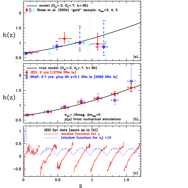
Figure 2: The cosmic expansion history (the dimensionless Hubble parameter $h(z)$) is measured in uncorrelated redshift bins from the Riess et al. (2004) “gold” sample (top panel) and from simulated future data (middle panel) for the NASA/JDEM mission concepts JEDI (solid points) and SNAP (dotted points). The measured $h(z)^{-1}$ in a given redshift bin is simply the sum of the comoving supernova distances in that bin, weighted by the corresponding solid curve in the bottom panel, which roughly speaking subtracts more nearby supernovae from more distant ones.

II.2 Averaging in redshift bins

The second step in our method is to average these noisy measurements ${\bf x}$ into minimum-variance measurements $y_{b}$ of the expansion history in some given redshift bins. For instance, the middle panel of Figure 2 shows an example with seven bins, $b=1,...,7$. Let the vector ${{\bf x}^{b}}$ denote the piece of the ${\bf x}$-vector corresponding to the $b^{\rm th}$ bin, and let ${{\bf N}_{b}}$ denote the corresponding covariance matrix. Our weighted average $y_{b}$ can then be written

$$y_{b}={{\bf w}^{b}}\cdot{{\bf x}^{b}}$$ (7)

for some weight vector ${{\bf w}^{b}}$ whose components sum to unity, i.e., $\sum_{i}w^{b}_{i}=1$ or equivalently ${\bf e}\cdot{{\bf w}^{b}}=1$, where ${\bf e}$ is a vector containing all ones; $e_{i}=1$. To find the best weight vector ${{\bf w}^{b}}$, we minimize the variance

$$\Delta y_{b}^{2}\equiv\langle y_{b}^{2}\rangle-\langle y_{b}\rangle^{2}={{\bf w}^{b}}^{t}{{\bf N}_{b}}{{\bf w}^{b}}$$ (8)

subject to the constraint that the weights add up to unity, i.e., that ${\bf e}\cdot{{\bf w}^{b}}=1$. This constrained minimization problem is readily solved with the Lagrange multiplier method, giving

$${{\bf w}^{b}}=\frac{{{\bf N}_{b}}^{-1}{\bf e}}{{\bf e}^{t}{{\bf N}_{b}}^{-1}{\bf e}},$$ (9)

and substituting this back into equation (8) gives the size of the corresponding error bar:

$$\Delta y_{b}=\left({\bf e}^{t}{{\bf N}_{b}}^{-1}{\bf e}\right)^{-1/2}.$$ (10)

The bottom panel in Figure 2 shows the seven weight vectors ${{\bf w}^{b}}$ (dotted) corresponding to the seven measurements $y_{b}$ in the middle panel (solid points). We will also refer to the weight vectors as window functions, since they show the contributions to our measurements from different redshifts. Note that each window function vanishes outside its redshift bin, and that all seven of them share a characteristic bump shape roughly corresponding to an upside-down parabola vanishing at the bin endpoints. To illustrate the $z$-range that each measurement probes, we plot it at the median of the window function with horizontal bars ranging from the 20th to the 80th percentile.

Since the measurements $y_{b}$ are linear combinations of the $x_{i}$ which are in turn linear combinations of the $r_{i}$, we can also reexpress our measurements directly as linear combinations of the original supernova comoving distances:

$$y_{b}=\sum_{i}{\tilde{w}}^{b}_{i}r_{i},$$ (11)

where the new window functions

$${\tilde{w}}^{b}_{i}\equiv{w^{b}_{i-1}\over\Delta z_{i-1}}-{w^{b}_{i}\over\Delta z_{i}}$$ (12)

would be essentially the negative derivative of the old window functions if all redshift intervals were the same. These new window functions are also plotted in the bottom panel of Figure 2 (solid “sawtooth” curves), and are seen to be roughly linear (as expected for a parabola derivative), effectively subtracting supernovae at the near end of the bin from those at the far end.

A major advantage of this method is its transparency and simplicity. If one fits some parametrized model of $H(z)$ to the SN Ia data by maximizing a likelihood function, then the resulting parameter estimates will be some complicated (and generically nonlinear) functions of all the data points $r_{i}$. In contrast, the measurement $y_{5}$ in our $5^{\rm th}$ bin in figure 2 (middle panel) is simply a linear combination of the comoving distance measurements for the supernovae in the $5^{\rm th}$ bin ($1.0<z_{i}<1.4$) as defined by the $5^{\rm th}$ window function in the bottom panel, so it is completely clear how each particular supernova affects the final result. In particular, the supernovae outside of this redshift range do not affect the measurement at all.

We conclude this section by discussing some details useful for the reader interested in applying our method in practice.

II.3 Creating uncorrelated redshift bins

We suggest discarding those $x_{i}$ straddling neighboring bins, i.e., whose two supernovae fall on either side of a bin boundary. For say 7 bins there are only 6 such numbers, so this involves a rather negligible loss. The advantage is that it ensures that two measurements $y_{b}$ and $y_{b^{\prime}}$ have completely uncorrelated error bars if $b\neq b^{\prime}$, since their window functions ${\tilde{w}}$ have no supernovae in common.

II.4 Flux averaging

To minimize the bias in the $H(z)$-measurement due to weak lensing, we use flux-averaging (Wang, 2000b; Wang & Mukherjee, 2004). Specifically, we compress the full supernova data set $r_{i}$ into a smaller number of of flux-averaged supernovae assigned to the mean redshift in each of a large number of bins of width $\Delta z$. We use $\Delta z=0.05$ for the current data and $\Delta z=0.005$ for the simulated data. Note that since we have assumed a Gaussian distribution in the magnitudes of SNe Ia at peak brightness, flux-averaging leads to a tiny bias of $-\sigma_{int}^{2}\,\ln 10/5$ mag (Wang, 2000a). We have removed this tiny bias in the data analysis.

As a side effect, this averaging in narrow bins makes the denominators $\Delta z_{i}$ roughly equal in equation (5), so that the only noticeable source of wiggles in the window functions in Figure 2 (bottom) is Poisson noise, i.e., that some of these narrow bins contain more supernovae than others. The method of course works without this averaging step as well. In that case, the window functions ${\bf w}$ wiggle substantially because of variations in the redshift spacing between supernovae, since very little weight is given to $x_{i}$ if $\Delta z_{i}$ happens to be tiny. However, we find that the supernova window functions ${\tilde{w}}$ remain rather smooth and well-behaved functions of redshift, as expected — two supernovae very close together with the same noise level $\sigma_{i}$ automatically get the same weight. This means that our method effectively averages such similar redshift supernovae anyway, even if we do not do so by hand ahead of time. The difference between flux averaging and this automatic averaging is simply that we average their fluxes rather than their comoving distances — these two types of averaging are not equivalent since the flux is a nonlinear function of the comoving distance.

III Results

Figure 2 shows the results of applying our method to both real data (top panel) and simulated data (middle panel), with the dimensionless expansion rate of the Universe $h(z)$ measured in between three and seven uncorrelated redshift bins.

The top panel uses the “gold” set of 157 SNe Ia published by Riess et al. (2004). The error bars are seen to be rather large, and consistent with a simple flat $\Omega_{m}=0.3$ concordance model where the dark energy is a cosmological constant. As was shown in Tegmark (2002) using information theory, the relative error bars on the cosmic expansion history $H(z)$ scale as

$${\Delta H\over H}\propto{\sigma\over N^{1/2}\Delta z^{3/2}},$$ (13)

for $N$ supernovae with noise $\sigma$. Here $\Delta z$ is the width of the redshift bins used, so one pays a great price for narrower bins: halving the bin size requires eight times as many supernovae. The origin of this $(\Delta z)^{-3/2}$-scaling is intuitively clear: the noise averages down as $(\Delta z)^{-1/2}$, and there is an additional factor of $(\Delta z)^{-1}$ from effectively taking the derivative of the data to recover $H(z)^{-1}$ from the integral in equation (5). The bottom panel in Figure 2 shows that the method effectively estimates this derivative by subtracting supernovae at the near end of the bin from those at the far end of the bin and dividing by $\Delta z$.

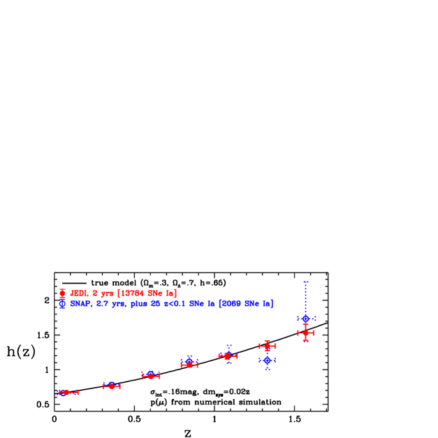
Figure 3: Same as Fig.2(b), but with a systematic bias of $dm_{sys}=0.02\,z$ from K-correction uncertainties added in addition to lensing noise computed from numerical simulations (Barber 2003 Barber et al. (2000)).

This means that for accurately measuring $H(z)$ and thereby the density history of the dark energy, numbers really do matter. For example, in order to measure the dark energy density function to 10% accuracy in seven uncorrelated redshift bins as in the middle panel of Figure 2 (with $\Delta z=0.243$), we need to have around 14,000 SNe Ia. We have simulated SN Ia data by placing supernovae at random redshifts, with the number of SNe Ia per 0.1 redshift interval given by a distribution. The intrinsic brightness of each SN Ia at peak brightness is drawn from a Gaussian distribution with a dispersion of $\sigma_{int}=0.16\,$ mag. As the fiducial cosmological model, we used a flat universe with $\Omega_{\Lambda}=0.7$.

We compare two mission concepts for the NASA/DOE Joint Dark Energy Mission (JDEM): the Joint Efficient Dark-energy Investigation (JEDI) (Wang et al., 2004b) and the Supernova Accelaration Probe (SNAP) (Aldering et al., 2004). For JEDI (solid points in Figure 2), the number of SNe Ia per 0.1 redshift interval is obtained by fitting the measured SN Ia rate as function of redshift (Cappellaro, Evans, & Turatto, 1999; Hardin et al., 2000; Dahlen et al., 2004) to a model assuming a conservative delay time between star formation and SN Ia explosion of 3.5 Gyrs. For SNAP (dotted points in Figure 2), the number of SNe Ia per 0.1 redshift interval is taken from Figure 9 in Aldering et al. (2004).

We consider two kinds of SN Ia systematic uncertainties: weak lensing due to intervening matter and a systematic bias due to K-corrections. We include the weak lensing effect by assigning a magnification $\mu$ drawn from a probability distribution $p(\mu)$, extracted using an improved version of the Universal Probability Distribution Function (UPDF) method (Wang, Holz, & Munshi, 2002) from the numerical simulations of weak lensing by Barber (2003) Barber et al. (2000). The total uncertainty in each SN Ia data point is $\sqrt{\sigma_{int}^{2}+\sigma_{lens}(z)^{2}}$, with $\sigma_{lens}(z)$ extracted from Barber (2003) Barber et al. (2000):

$$\sigma_{lens}(z)\simeq 0.00311+0.08687z-0.00950z^{2}$$ (14)

We consider a systematic bias of $\Delta m_{\rm sys}=0.02z$ due to K-corrections following Wang & Garnavich (2001).

We did not include the systematic bias due to K-corrections in Fig.2, in order to compare the real data (Riess et al., 2004) and simulated data on an equal footing.

In Fig. 3, we show the effect of adding the systematic bias due to K-corrections in addition to the weak lensing noise. Comparing Fig. 3 with Fig. 2 (b), we see that the systematic bias does not have a significant effect on the uncorrelated estimates of $H(z)$. This is because our method effectively reduces a global systematic bias into a local bias with a much smaller amplitude (see Sec. 2).

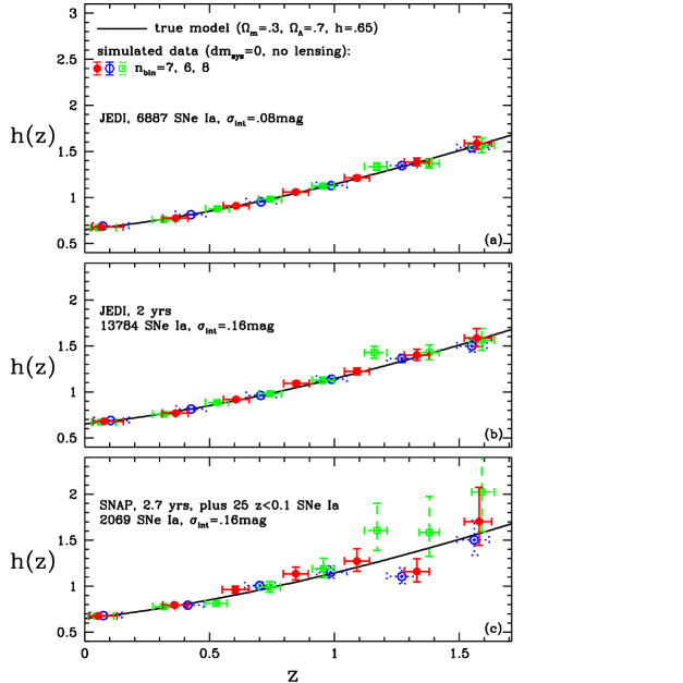
Figure 4: How the recovery of the cosmic expansion history $h(z)$ depends on the number of redshift bins, assuming no systematic bias and no lensing. (a) Half of JEDI data, with a reduced intrinsic scatter of $\sigma_{int}=0.08\,$ mag. (b) All of JEDI data, with $\sigma_{int}=0.16\,$ mag. (c) All of SNAP data (plus 25 SNe Ia at $z<0.1$), with $\sigma_{int}=0.16\,$ mag.

Figure 4 shows how the recovery of the cosmic expansion history $h(z)$ depends on the number of redshift bins (6, 7 and 8), assuming no systematic bias and no lensing, and agrees well with the theoretical $(\Delta z)^{3/2}$ scaling. Contrasting current and future data with roughly the same redshift binsize for both ($n_{bin}$=5 for current data, and $n_{bin}$=7 for the simulated data) shows that JEDI shrinks the error bars by more than an order of magnitude, so the potential improvement with a successful JDEM would be dramatic.

Figure 4 compares three different data sets: (a) Half of the JEDI data, with a reduced intrinsic scatter of $\sigma_{int}=0.08\,$ mag from sub-typing. (b) All the JEDI data, with $\sigma_{int}=0.16\,$ mag. (c) All the SNAP data (plus 25 SNe Ia at $z<0.1$), with $\sigma_{int}=0.16\,$ mag.

Note that since the measured quantity $h(z)^{-1}$ typically is not a straight line, the measured average of this curve over a redshift bin will generally lie either slightly above of below the curve at the bin center. Figure 2 shows that this bias is substantially smaller than the measurement uncertainties, since $h(z)$ and $h(z)^{-1}$ are rather well approximated by straight lines over the narrow redshift bins that we have used.

A second caveat when interpreting our figures is that the absolute calibration of SN Ia is not perfectly known — changing this simply corresponds to multiplying the function $h(z)$ by a constant, i.e., to scaling the measured curve vertically.

IV Discussion

We have presented a method for measuring the cosmic expansion history $H(z)$ in uncorrelated redshift bins, and applied it to current and simulated supernova Ia data assuming spatial flatness. Whereas previously proposed approaches involve “black box” parameter fitting, this method is transparent and simple to interpret: the measurement of $H(z)^{-1}$ in a redshift bin is simply a linear combination of the measured comoving distances for supernovae in that bin, with weights that roughly correspond to subtracting closer supernovae from more distant ones. Such transparency is particularly helpful for understanding how systematic errors in the input affect the output. For instance, a constant systematic dimming throughout a redshift bin will leave that measurement unaffected.

This method is useful for understanding the nature of dark energy, since the dark energy density history follows from this expansion history $H(z)$ if the matter density parameter $\Omega_{m}$ can be accurately measured from other data (e.g., the cosmic microwave background, galaxy clustering and gravitational lensing). We found the Riess et al. (2004) “gold” sample to be consistent with the “vanilla” concordance model where the dark energy is a cosmological constant, but that much larger numbers of supernovae are needed for true precision tests of the nature of dark energy. We obtain good agreement with the results of Daly03 ; Daly & Djorgovski (2004) — the fact that two quite different techniques give consistent answers indicates a reassuring robustness to method and data details.

Looking towards the future, we compare two mission concepts for the NASA/DOE Joint Dark Energy Mission (JDEM), the Joint Efficient Dark-energy Investigation (JEDI) and the Supernova Accelaration Probe (SNAP), using simulated data including the effect of weak lensing and bias from K-corrections. Estimating $H(z)$ in seven uncorrelated redshift bins, we find that both provide dramatic improvements over the present state-of-the art: JEDI can measure $H(z)$ to about 10% accuracy, and SNAP can measure $H(z)$ to 30-40% accuracy (Figure 2).

Our results show that numbers do matter. For example, in order to measure the cosmic expansion history to 10% accuracy in seven uncorrelated redshift bins (with $\Delta z=0.243$), we need to have around 14,000 SNe Ia (as expected from two years of JEDI data), assuming a dispersion of 0.16 magnitudes in SN Ia peak brightness (Figure 2). Estimating $H(z)$ to 10% in smaller uncorrelated redshift bins will require an even larger number of SNe Ia (if a significant reduction in intrinsic dispersion is not assumed for a sizable fraction of the SNe Ia), which will be difficult to obtain in a feasible two-year space mission. Also, $H(z)$ estimated in $\Delta z=0.243$ redshift bins (for $0\leq z\leq 1.7$) to 10% accuracy will give us a powerful means to differentiate between a cosmological constant and dark energy models which are not fine-tuned to mimic a cosmological constant. A sample with a large number of SNe Ia allows tighter calibration of SNe Ia as standard candles and subtyping of SNe Ia to reduce diversity. This may yield a smaller set of SNe Ia with substantially smaller intrinsic dispersion, which can lead to more robust and stable estimates of the expansion history of the universe (Figure 4a). If the subtyping works well in reducing the intrinsic dispersion of SNe Ia, we can expect to be able to measure $H(z)$ in more than seven redshift bins to 10% accuracy for $0\leq z\leq 1.7$ (Figure 4a).

A precise measurement of the cosmic expansion history as a free function of cosmic time to 10% accuracy would represent a dramatic improvement in our knowledge about dark energy. Our results suggest that a JDEM can achieve this scientific goal.

Acknowledgements We thank David Branch, Peter Garnavich, and Ruth Daly for helpful comments. This work was supported by NSF CAREER grants AST-0094335 (YW) and AST-0134999 (MT), NASA grant NAG5-11099 and fellowships from the David and Lucile Packard Foundation and the Cottrell Foundation (MT).

References

- Riess et al. (1998) Riess, A. G, et al., 1998, Astron. J., 116, 1009
- Perlmutter et al. (1999) Perlmutter, S. et al., 1999, ApJ, 517, 565
- Freese et al. (1987) Freese, K., Adams, F.C., Frieman, J.A., and Mottola, E., Nucl. Phys. B287, 797 (1987).
- Linde (1987) Linde A D, “Inflation And Quantum Cosmology,” in Three hundred years of gravitation, (Eds.: Hawking, S.W. and Israel, W., Cambridge Univ. Press, 1987), 604-630.
- Peebles & Ratra (1988) Peebles, P.J.E., and Ratra, B., 1988, ApJ, 325, L17
- Wetterich (1988) Wetterich, C., 1988, Nucl.Phys., B302, 668
- Frieman et al. (1995) Frieman, J.A., Hill, C.T., Stebbins, A., and Waga, I., 1995, PRL, 75, 2077
- Caldwell, Dave & Steinhardt (1998) Caldwell, R., Dave, R., & Steinhardt, P.J., 1998, PRL, 80, 1582
- Sahni & Habib (1998) Sahni, V., & Habib, S., 1998, PRL, 81, 1766
- Parker & Raval (1999) Parker, L., and Raval, A., 1999, PRD, 60, 063512
- Boisseau et al. (2000) Boisseau, B., Esposito-Farèse, G., Polarski, D. & Starobinsky, A. A. 2000, Phys. Rev. Lett., 85, 2236
- Deffayet (2001) Deffayet, C., 2001, Phys. Lett. B, 502, 199
- Mersini, Bastero-Gil, & Kanti (2001) Mersini, L., Bastero-Gil, M., & Kanti, P., 2001, PRD, 64, 043508
- Freese & Lewis (2002) Freese, K., & Lewis, M., 2002, Phys. Lett. B, 540, 1
- Carroll et al. (2004) Carroll, S M, de Felice, A, Duvvuri, V, Easson, D A, Trodden, M & Turner, M S, Phys.Rev. D71 (2005) 063513, astro-ph/0410031
- Padmanabhan (2003) Padmanabhan, T., 2003, Phys. Rep., 380, 235
- Peebles & Ratra (2003) Peebles, P.J.E., & Ratra, B., 2003, Rev. Mod. Phys., 75, 559
- Choudhury & Padmanabhan (2004) Choudhury, T. R., & Padmanabhan, T. 2004, Astron.Astrophys. 429 (2005) 807, astro-ph/0311622
- Chen & Ratra (2004) Chen, G., & Ratra, B. 2004, Astrophys.J. 612, L1
- (20) Daly, R. A. & Djorgovski, S. G. 2003, ApJ, 597, 9
- Daly & Djorgovski (2004) Daly, R. A. & Djorgovski, S. G. 2004, ApJ, 612, 652
- Dicus & Repko (2004) Dicus, D.A., & Repko, W.W. 2004, Phys.Rev. D70, 083527
- Hannestad & Mortsell (2004) Hannestad, S., & Mortsell, E. 2004, JCAP, 0409, 001
- Simon, Verde, & Jimenez (2004) Simon, J., Verde, L., & Jimenez, R. 2004, astro-ph/0412269
- Wang & Tegmark (2004) Wang, Y., & Tegmark, M. 2004, Phys. Rev. Lett., 92, 241302
- Jassal, Bagla, & Padmanabhan (2005) H.K.Jassal, J.S.Bagla, T.Padmanabhan, 2005, MNRAS, 356, L11, astro-ph/0404378
- Alam, Sahni, & Starobinsky (2004) Alam, U., Sahni, V., & Starobinsky, A. A. 2004, JCAP, 0406, 008,
- Capozziello, Cardone, & Francaviglia (2004) Capozziello, S., Cardone, V.F., & Francaviglia, M., 2004, astro-ph/0410135
- Huterer & Cooray (2004) Huterer, D., & Cooray, A., Phys.Rev. D71 (2005) 023506, astro-ph/0404062
- Feng et al. (2004) Feng, B., Li, M., Piao, Y.-S. Zhang, X., astro-ph/0407432
- Wang et al. (2004a) Wang, Y., Kratochvil, J.M., Linde, A., & Shmakova, M. 2004, astro-ph/0409264, JCAP in press
- Wang & Garnavich (2001) Wang, Y., and Garnavich, P. 2001, ApJ, 552, 445
- Wang & Lovelace (2001) Wang, Y., and Lovelace, G. 2001, ApJ, 562, L115
- Wang & Freese (2004) Wang, Y., and Freese, K., astro-ph/0402208
- Maor, Brustein, & Steinhardt (2002) Maor, I., Brustein, R., & Steinhardt, P. J., 2002, PRL, 86, 6
- Bassett, Corasaniti, & Kunz (2004) Bassett, B. A., Corasaniti, P. S., Kunz, M. 2004, Astrophys.J. 617, L1-L4
- Tegmark (2002) Tegmark, M. 2002, Phys. Rev. D66, 103507
- Wang (2000b) Wang, Y. 2000b, Astrophys. J. , 536, 531
- Wang & Mukherjee (2004) Wang, Y. and Mukherjee, P. 2004, ApJ, 606, 654
- Riess et al. (2004) Riess, A. G., et al. 2004, ApJ, 607, 665
- Wang (2000a) Wang, Y. 2000a, ApJ, 531, 676
- Barber et al. (2000) Barber, A.J., et al. 2000, MNRAS, 319, 267; Barber, A.J. 2003, private communication.
- Wang et al. (2004b) Wang, Y., et al. 2004 (the JEDI Team), BAAS, 36, 5, 1560. See also http://jedi.nhn.ou.edu/.
- Aldering et al. (2004) Aldering, G., et al., astro-ph/0405232
- Cappellaro, Evans, & Turatto (1999) Cappellaro, E.; Evans, R.; & Turatto, M. 1999, A & A, 351, 459
- Hardin et al. (2000) Hardin, D., et al. 2000, A & A, 362, 419
- Dahlen et al. (2004) Dahlen, T., et al. 2004, ApJ, 613, 189
- Wang, Holz, & Munshi (2002) Wang, Y., Holz, D.E., and Munshi, D. 2002, ApJ, 572, L15