An XMM-Newton Observation of Abell 2597

Abstract

We report on a 120$\mathrm{\,ks}$ XMM-Newton observation of the galaxy cluster Abell 2597. Results from both the European Photon Imaging Camera (EPIC) and the Reflection Grating Spectrometer (RGS) are presented. From EPIC we obtain radial profiles of temperature, density and abundance, and use these to derive cooling time and entropy. We illustrate corrections to these profiles for projection and point spread function (PSF) effects. At the spatial resolution available to XMM-Newton, the temperature declines by around a factor of two in the central 150$\mathrm{\,kpc}$ or so in radius, and the abundance increases from about one-fifth to over one-half solar. The cooling time is less than 10$\mathrm{\,Gyr}$ inside a radius of 130$\mathrm{\,kpc}$. EPIC fits to the central region are consistent with a cooling flow of around 100 solar masses per year. Broad-band fits to the RGS spectra extracted from the central 2$\mathrm{\,arcmin}$ are also consistent with a cooling flow of the same magnitude; with a preferred low-temperature cut-off of essentially zero. The data appear to suggest (albeit at low significance levels below formal detection limits) the presence of the important thermometer lines from Fe 17 at 15, 17 Å rest wavelength, characteristic of gas at temperatures $\sim 0.3\mathrm{\,keV}$. The measured flux in each line is converted to a mass deposition estimate by comparison with a classical cooling flow model, and once again values at the level of 100 solar masses per year are obtained. These mass deposition rates, whilst lower than those of previous generations of X-ray observatories, are consistent with those obtained from UV data for this object. This raises the possibility of a classical cooling flow, at the level of around 100 solar masses per year, cooling from 4$\mathrm{\,keV}$ by more than two orders of magnitude in temperature.

1 Introduction

Abell 2597 is a relatively nearby ($z\approx 0.08$), Abell richness class 0 cluster of galaxies. Rich in features, it has been studied extensively in many wavebands.

The central cD galaxy contains the radio source PMN J2323-1207 (PKS B2322-12) (Wright & Otrupcek, 1990; Griffith et al., 1994). The total flux density of this source is $\sim 1.7\mathrm{\,Jy}$ at 1.5$\mathrm{\,GHz}$ (McNamara et al., 2001; Owen et al., 1992), and $\sim 0.3\mathrm{\,Jy}$ at 5.0$\mathrm{\,GHz}$ (Ball et al., 1993), implying a fairly steep spectral index $\alpha=-1.3$ ($S_{\mathrm{\nu}}\propto\nu^{\alpha}$). The source is physically small, $\sim 7\times 5,5\times 2\mathrm{\,arcsec}$ at 1.5, 5.0$\mathrm{\,GHz}$ respectively. The source is only moderately resolved at these frequencies, but at the higher frequency has an elongated appearance suggesting a double-lobed structure. At 8.44$\mathrm{\,GHz}$ (Sarazin et al., 1995), the source is resolved into a nucleus and two lobes ($\sim 5\mathrm{\,arcsec}$ across), orientated roughly NE–SW. A jet is clearly seen leading from the nucleus on the SW. This jet undergoes a sharp ($\sim 90\mathrm{\,{}^{\circ}}$) bend about 0.5$\mathrm{\,arcsec}$ from the nucleus. Assuming a typical spectral index for the jets of $-0.7$, the inferred lobe spectral index is $\approx-1.5$, suggestive of confinement and synchrotron ageing. Very Long Baseline Array (VLBA) 1.3, 5.0$\mathrm{\,GHz}$ observations of the central 0.3$\mathrm{\,arcsec}$ (Taylor et al., 1999) show an inverted spectrum ($\alpha=0.6$) core, together with straight, symmetric jets emanating from both sides.

Abell 2597 has previously been observed in X-rays by various observatories, for example: Einstein (Crawford et al., 1989); ROSAT (Sarazin et al., 1995; Sarazin & McNamara, 1997; Peres et al., 1998); ASCA (White, 2000); Chandra (McNamara et al., 2001); XMM-Newton (Still & Mushotzky, 2002). Traditionally, it has been classified as a moderately strong cooling flow (e.g. Fabian, 1994) cluster, with inferred X-ray mass deposition rate ($\mathrm{\,\mathrm{\,M_{\odot}}}$$\mathrm{\,yr^{-1}}$): $270\pm 41$ (ROSAT PSPC; Peres et al., 1998, $r_{\mathrm{cool}}=152^{+67}_{-58}\mathrm{\,kpc}$); $259^{+176}_{-178}$ (ASCA; White, 2000).

A short ($\sim 20\mathrm{\,ks}$ of good time) Chandra observation (McNamara et al., 2001) highlighted the interaction between the radio source and the X-ray gas, through the presence of so-called ‘ghost cavities’ of low surface brightness, seemingly coincident with spurs of low frequency ($1.4\mathrm{\,GHz}$) radio emission. Such brightness depressions are believed to be buoyantly rising bubbles (e.g. Bîrzan et al., 2004) associated with a prior ($\sim 10^{8}\mathrm{\,yr}$ previously, in this case) outburst of the central radio source. The small physical size of the radio source means, however, that these issues are not amenable to study with XMM-Newton, given its $\sim 5\mathrm{\,arcsec}$ point spread function (PSF).

In the Chandra and XMM-Newton era of high spatial and spectral resolution, the cooling flow model is undergoing re-interpretation. The cause is quite simply an absence (or at best a severe weakness) of the spectral features expected from gas at the low-end ($\la 1\mathrm{\,keV}$, say; though there does not appear to be a fixed absolute cut-off) of the X-ray temperature regime in the observed spectra of cluster central regions. Reductions in temperature by factors of a few (e.g. Kaastra et al., 2004) with radius are seen. The expected emission lines for several important low-temperature species (e.g. the Fe 17 15 and 17 Å lines) do not seem to be present at the levels predicted by simple models. This is a trend that appears to be repeated in many clusters that have traditionally been thought to harbour cooling flows (e.g. Peterson et al., 2003). Many explanations (e.g. Fabian et al., 2001; Peterson et al., 2001) for this effect have been put forward; some involving suppression of the gas cooling, some involving departures from standard collisionally-ionized radiative cooling. After a flirtation with thermal conduction (but see e.g. Soker, 2003), theoretical studies at present seem to be concentrated on some form of distributed heating from a central AGN (e.g. Vecchia et al., 2004; Reynolds et al., 2005; Ruszkowski et al., 2004), effected by buoyant plasma bubbles.

Observations at ultra-violet (UV) wavelengths suggest that Abell 2597 may be a particularly interesting object for study in light of these issues. Abell 2597, together with the $z=0.06$ cluster Abell 1795, was observed with the Far Ultraviolet Spectroscopic Explorer (FUSE; Moos et al., 2000) mission by Oegerle et al. (2001). FUSE is sensitive to the O 6 1032, 1038 Å resonance lines, which are strong diagnostics of thermally radiating gas at temperatures $\sim$ $3\times 10^{5}$$\mathrm{\,K}$. In a traditional cooling flow model, in which the ultimate fate of the hot gas is to cool to very low temperatures, strong UV emission is expected in such lines as gas cools out of the X-ray temperature regime; thereby potentially forming a bridge between the hot, X-ray emitting gas and the cool, $\mathrm{H}\alpha$ (see below) radiating gas. O 6 1032 Å emission was detected in Abell 2597, with an inferred luminosity $3.6\times 10^{40}$$\mathrm{\,erg}$$\mathrm{\,s^{-1}}$. Using simple cooling-flow theory, Oegerle et al. (2001) calculate the associated mass flow-rate as 40$\mathrm{\,\mathrm{\,M_{\odot}}}$$\mathrm{\,yr^{-1}}$ (within the effective radius of the FUSE aperture at this redshift, $\sim 40\mathrm{\,kpc}$), for an intermediate case between the limits of isobaric and isochoric cooling. The ROSAT HRI mass deposition rate of Sarazin et al. (1995), $\approx 330\mathrm{\,\mathrm{\,M_{\odot}}}\mathrm{\,yr^{-1}}$ within a cooling radius (defined by $t_{\mathrm{cool}}<10\mathrm{\,Gyr}$) $\approx 130\mathrm{\,kpc}$, is around three times larger (applying a simple linear $\dot{M}\propto r$ scaling). The weakness of cluster cooling flows in comparison to the predictions of the traditional model is thus again demonstrated, but extended down to the UV regime. This under-luminosity at UV temperatures may be contrasted with the situation at $\mathrm{H}\alpha$ temperatures, where the Abell 2597 emission nebula (see below), like other such nebulae, is over-luminous, even when compared to classical, high X-ray mass deposition rates (Voit & Donahue, 1997).

In contrast, Abell 1795 was not detected in O 6. Similarly, Lecavelier des Etangs et al. (2004), also using FUSE, were unable to detect O 6 emission from either of the low redshift ($z\approx 0.07$), low Galactic column ($N_{\mathrm{H}}\sim 4\times 10^{20}\mathrm{\,cm^{-2}}$), rich clusters Abell 2029 and Abell 3112. These results highlight the apparently unusual (within the currently favoured non-cooling flow paradigm) nature of Abell 2597, and motivate a more detailed X-ray study of its properties.

The central ($\sim 15\mathrm{\,arcsec}$ in diameter) regions of Abell 2597 harbour an optical emission line nebula, as is often (and exclusively) the case in cooling flow clusters. The $\mathrm{H}\alpha+[\text{N\,\textsc{2}}]$ luminosity is $2.7\times 10^{42}\mathrm{\,erg}\mathrm{\,s^{-1}}$, making it among the most luminous in the sample of Heckman et al. (1989). The $\mathrm{H}\alpha$ luminosity is many ($\sim 300$) times greater than that expected from extrapolating the classical $\sim 10^{7}\mathrm{\,K}$ X-ray mass flow rates down to $\sim 10^{4}\mathrm{\,K}$, a general feature of such nebulae. The discrepancy is made even worse if the relative sizes of the nebulae and X-ray cooling regions are taken into account. The deep optical spectra of Voit & Donahue (1997) reveal that the Abell 2597 nebula has $T\sim 10^{4}\mathrm{\,K}$, $Z\sim 0.5\mathrm{\,\mathrm{\,Z_{\odot}}}$, $n_{\mathrm{e}}\sim 200\mathrm{\,cm^{-3}}$, and is significantly reddened by (intrinsic, owing to the low Galactic column) dust. The low inferred column density $N_{\mathrm{\text{H\,\textsc{2}}}}\approx 3\times 10^{19}\mathrm{\,cm^{-2}}$ relative to that of H 1 suggests that thin ionized H 2 layers surround cold neutral H 1 cores. The nebula has a low ionization parameter, most species being only singly ionized. Photoionization from hot stars is the only ionization mechanism not ruled out by the observations, but even the hottest O stars (in isolation) would not be able to heat the nebula to the observed temperature. Some form of heat transfer from the intracluster medium (ICM) may supply a comparable amount of energy to the nebula.

The core of the central cD exhibits a significant blue optical excess (e.g. McNamara & O’Connell, 1993; Sarazin et al., 1995). HST observations (Koekemoer et al., 1999) resolve this excess into continuum emission around and across the radio lobes, and several knots to the south-west. Line-dominated (thereby not optical synchrotron or inverse Compton in origin) excess appears in bright arcs around the edge of the radio lobes, and more diffusely across the lobe faces. Such geometry is suggestive of an emission shell surrounding the radio lobes. A bright optical knot is also seen coincident with the southern radio hot-spot, consistent with a massive clump responsible for the deflection of the southern jet. The central region also shows strong dust obscuration, resolved into several large (several hundred parsecs) regions.

In the infra-red, vibrational molecular hydrogen emission lines characteristic of $\sim$ 1000–2000$\mathrm{\,K}$ collisionally ionized gas have been detected from the innermost $\sim 3\mathrm{\,arcsec}$ of the central cluster galaxy (Falcke et al., 1998; Donahue et al., 2000; Edge et al., 2002). As with the optical nebula, there is too much emission as compared to the expectation from even an inordinately massive classical cooling flow, and yet too little mass for this to be the final reservoir of a standard, long-lived flow. Furthermore, the molecular gas is dusty, and therefore unlikely to be the direct condensate of the hot ICM (where dust is rapidly destroyed). Again as with the optical light, there is a complex filamentary structure that seems to be spatially associated with the radio source. The optical and infra-red properties are both consistent with UV heating of the gas by a population of young, hot stars (Donahue et al., 2000) (SFR $\sim$ few $\mathrm{\,\mathrm{\,M_{\odot}}}\mathrm{\,yr^{-1}}$). Abell 2597 also has a possible CO detection (Edge, 2001); indicative of very cold, molecular gas.

The Galactic column density in the direction of Abell 2597 ($l=65.4$, $b=-64.8$) has the relatively low value $2.5\times 10^{20}$$\mathrm{\,cm^{-2}}$ (Dickey & Lockman, 1990; Stark et al., 1992). Recently, Barnes & Nulsen (2003) have shown that the $5\sigma$ limit on any fluctuation in the foreground H 1 column in this direction, on scales $\sim 1\mathrm{\,arcmin}$, is $0.43\times 10^{20}$$\mathrm{\,cm^{-2}}$ (17 per cent).

Intrinsic H 1 21$\mathrm{\,cm}$ absorption towards the central radio source was detected by O’Dea et al. (1994). A narrow ($\sim 200\mathrm{\,km}\mathrm{\,s^{-1}}$), redshifted ($\sim 300\mathrm{\,km}\mathrm{\,s^{-1}}$), spatially unresolved component coincident with the nucleus is inferred to be a gas clump falling onto the cD. A broad ($\sim 400\mathrm{\,km}\mathrm{\,s^{-1}}$), spatially extended ($\sim 3\mathrm{\,arcsec}$, i.e. the size of the radio source) component at the systemic velocity is consistent with being associated with the (hence photon bounded) $\mathrm{H}\alpha$. The inferred column densities and masses for the narrow and broad components are $N_{\mathrm{H}}\sim\{8.2,4.5\}\times 10^{20}T_{\mathrm{s}}\mathrm{\,cm^{-2}}$; $M\sim\{3.5,7\}\times 10^{7}T_{\mathrm{s}}\mathrm{\,\mathrm{\,M_{\odot}}}$; with $T_{\mathrm{s}}$ the spin temperature in units of 100$\mathrm{\,K}$. Intrinsic, redshifted H 1 was also seen in the VLBA observations of Taylor et al. (1999), and interpreted as a turbulent, inwardly streaming, atomic torus (scale height $\la 20\mathrm{\,pc}$) centred on the nucleus.

Our chosen cosmology has $H_{0}=50$$\mathrm{\,km}$$\mathrm{\,s^{-1}}$$\mathrm{\,Mpc^{-1}}$, $\Omega_{\mathrm{M}}=1.0$, and $\Omega_{\Lambda}=0.0$. Adopting a redshift $z=0.0822$ (see Section 5.2.1), the luminosity distance is $D_{\mathrm{L}}=503\mathrm{\,Mpc}$, the angular diameter distance is $D_{\mathrm{A}}=429\mathrm{\,Mpc}$, and the angular length scale is 2.08$\mathrm{\,kpc}$$\mathrm{\,arcsec^{-1}}$. Data processing was carried out using the XMM-Newton Science Analysis System (SAS) version 5.4.1 (aka xmmsas_20030110_1802). Spectral analyses employed xspec version 11.3. Unless otherwise stated, quoted uncertainties are $1\sigma$ (68 per cent) on a single parameter.

2 EPIC data reduction

Abell 2597 was observed by XMM-Newton on 2003 June 27–28 (observation ID 0147330101), during revolution 0650. The nominal length of the observation was 120$\mathrm{\,ks}$, unfortunately the exposure was heavily affected by background flaring (see Fig. 1). The thin optical blocking filter was applied to the European Photon Imaging Camera (EPIC). The MOS (Turner et al., 2001) and pn (Strüder et al., 2001) detectors were both operated in Full Frame mode.

EPIC events files were regenerated from the Observation Data Files (ODFs) using the SAS meta-tasks epchain and emchain. For emchain, standard options were used, except that bad pixel detection was switched on. epchain was run in two steps in order to merge in the instrument house-keeping Good Time Interval (GTI) data (which are otherwise ignored) before the final events list was created.

2.1 Background filtering and subtraction

The EPIC background is comprised of a number of components: proton, particle, photon. Soft protons in the Earth’s magnetosphere scatter through the mirror system, and are responsible for periods of intense background flaring, where the instrument count rate can rise by orders of magnitude. Such intervals can only be dealt with by excising them from further analysis using a rate-based GTI filtering. Energetic charged particles that pass through the detector excite fluorescent emission lines in several of the constituent components. The strong spatial variation of some components of this emission (Freyberg et al. 2002a, Freyberg et al. 2002b, Lumb 2002) makes it preferable to extract a background from the same region of the detector as the source. For the analysis of extended sources, the use of blank-sky background templates (Lumb, 2002) is therefore to be desired.

For Abell 2597, cluster emission is detected up to around 8 and 9$\mathrm{\,keV}$ in the MOS and pn respectively. The pn exhibits strong fluorescence lines of Ni, Cu and Zn around 8$\mathrm{\,keV}$. The only non-negligible fluorescent line visible in the pn data below 8$\mathrm{\,keV}$ is the 1.5$\mathrm{\,keV}$ Al line. Unlike the Cu (for example) line, this line does not vary spatially over the detector (Freyberg et al., 2002b), since it originates in the camera housing. Cutting off the spectra at 7.3$\mathrm{\,keV}$ removes very few counts, and means that the only background line remaining in the pn is not spatially varying. This frees us from the need to extract background spectra from the same spatial region of the pn detector, i.e. enables us to use a local background. This is desirable because it removes the vagaries of scaling and varying cosmic background necessarily associated with the use of a blank-sky background (see below); and it allows us greater freedom in the filtering of background flares. Additionally, comparison of the off-source pn spectra for the Abell 2597 and blank-sky fields reveals that the 8$\mathrm{\,keV}$ fluorescence lines are shifted to a lower energy by about 20$\mathrm{\,eV}$ in the latter. This almost certainly represents a change in calibration between the processing of the blank-sky templates and our re-processing of the ODFs for Abell 2597 (the effect of such a shift would of course be largely restricted to an increase in $\chi^{2}$ in those channels lying around the fluorescent line energies).

The only significant fluorescent lines in the MOS data are the Al and Si lines at 1.5 and 1.7$\mathrm{\,keV}$ respectively (the Cr, Mn, and Fe lines around 6$\mathrm{\,keV}$ are seen to be negligible). Both of these features exhibit strong spatial variation (Lumb, 2002) over the MOS field of view (hereinafter fov). Using a local background for the MOS is therefore not as viable a proposition as it is for the pn.

In order to be able to make use of the blank-sky EPIC background templates of Lumb (2002), we use the same form of filtering process as employed in the construction of those files. That is, we make a light-curve (e.g. Fig. 1) in 100$\mathrm{\,s}$ time bins of the high energy (PI $>$ 10000) single pixel (PATTERN == 0) events across the whole detector. The standard XMM event selection flags #XMMEA_EM and #XMMEA_EP are applied for the MOS and pn respectively (these exclude cosmic rays, events in bad frames, etc.).

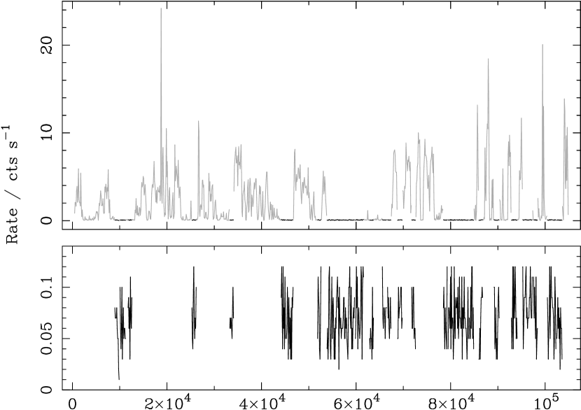
Figure 1: MOS2 light curve formed from 100$\mathrm{\,s}$ time bins. Upper panel: total exposure, with rejected periods of high count-rate in grey, accepted periods in black. Lower panel: only the selected Good Time Interval (GTI) is shown.

Our preferred filtering method is to form a histogram of the number of events in the 100$\mathrm{\,s}$ time-bins of the light curve, fit the core of the distribution (i.e. ignoring the high count-rate tail) with a Gaussian, and exclude periods where the count-rate lies more than $n\sigma$ away from the mean. Unfortunately, for MOS1 (and the pn, but this is not an issue since we use a local background in this case) the $2\sigma$ count-rate thresholds lie above the filtration limits used in the creation of the background events templates (0.2 and 0.45$\mathrm{\,ct}$$\mathrm{\,s^{-1}}$ for the MOS and pn respectively). In order to make use of the MOS1 background template we therefore apply the same absolute count-rate filtering to this instrument as was used to make the background events file. For MOS2, the $2\sigma$ count-rate threshold is 0.13$\mathrm{\,ct}$$\mathrm{\,s^{-1}}$, and this absolute value is used to filter both the observation events file, and to re-filter the background template events file to the same level. For the pn, the $2\sigma$ count-rate threshold is 0.54$\mathrm{\,ct}$$\mathrm{\,s^{-1}}$.

We strengthen the filtering by requiring that all GTIs be at least 10 minutes long. The GTI files are aligned on the frame boundaries of the relevant events files before being applied. The mean remaining ONTIME of the events files after filtering in this way are 39 (pn), 37 (MOS1), and 38$\mathrm{\,ks}$ (MOS2).

It is known that the particle background can vary from observation to observation at around the ten per cent level (Freyberg et al., 2002a). We therefore scale the products (images and spectra) of the blank-sky MOS events file before they are used to correct the source products. The scaling factor is obtained from the ratio of the count-rates outside the fov, where the only events should be the result of particle-induced fluorescence rather than from actual photons passing through the mirror system. In detail, we find the number of counts remaining in the GTI-filtered data after applying the evselect filtering criterion #XMMEA_16 && FLAG & 0x766a0f63 == 0 && PI in [200:12000] && PATTERN $<=$ 12, where the flag expression selects events outside the MOS fov but with no other non-zero flag settings. Combining this figure with the exposure time gives an out-of-fov count-rate which is used to normalize the background template products. In this way, we obtain scaling factors of 1.02 and 0.91 for the MOS1 and MOS2 backgrounds respectively. To allow for some uncertainty in the normalization, we assign a 10 per cent systematic error to the blank-sky products, which is added in quadrature to the statistical errors.

The SAS task attcalc was used to reproject the blank-sky templates to the same sky position as the Abell 2597 observation, so that the same sky coordinate selection expressions could be applied to both the science and background fields.

Below 5$\mathrm{\,keV}$ or so, the cosmic X-ray background (CXB) dominates (Lumb, 2002) over the internal camera background. If there were no significant variation of the CXB over the sky, then the blank-sky templates would also represent this background component. To allow for any changes in the CXB in the region of the target, a so-called double background subtraction approach can be used. The large field of view of XMM-Newton, together with the redshift of Abell 2597, result in significant areas of the detectors being essentially free from cluster emission. This enables us to examine the background spectrum from such regions and compare it with those of the (scaled) blank-sky templates extracted from the same detector region. For this purpose we extracted spectra from an annulus lying between 7 and 10$\mathrm{\,arcmin}$ (avoiding regions near the edge of the fov) from the cluster centre, which we take to be located at the emission peak, in sky coordinates $(X,Y)=(23720.5,23720.5)$. Non-ICM sources in this region were excluded with circular masks of radius at least 30$\mathrm{\,arcsec}$. The BACKSCAL FITS header keys were corrected for the area so removed.

Initial comparison of the spectra extracted from this region of the Abell 2597 field reveals that the agreement with the blank-sky spectra scaled according to the out-of-fov count-rates is good; despite the relatively poor quality of the science observation as a whole (i.e. the heavy background flaring). There is something of a slight excess of soft ($\la 2\mathrm{\,keV}$) counts in the Abell 2597 field, but not to any great degree.

In summary, we use a local (extracted from 7–10$\mathrm{\,arcmin}$ in radius) background for the pn. For the MOS, we use the blank-sky templates to deal with the spatially varying Si and Al background lines, corrected by a double-background subtraction approach to account for any (minor) variance in CXB between the science and background fields. For the MOS, we make use of single, double, triple, and quadruple pixel events (i.e. PATTERN $\leqslant$ 12). For the pn, we use single and double events (PATTERN $\leqslant$ 4). In both cases only events with FLAG == 0 are considered.

2.2 Out of time events

When the pn is operated in Full Frame mode, as is the case here, bright sources can be significantly affected by so-called out of time (OOT) events. These are caused by photons which arrive while the CCD is being read out (charge shifted along columns towards the readout node). Such events are assigned a wrong RAWY coordinate and hence an improper CTI (charge transfer inefficiency) correction. In an uncorrected image, the OOT events due to a strong source are visible as a bright streak smeared out in RAWY. OOT events act to broaden spectral features.

OOT events can only be corrected for in a statistical sense. We follow the standard procedure of re-running the SAS meta-task epchain with the option withoutoftime=y passed to the epevents task. This generates an events file that consists entirely of OOT events, distributed over the range of RAWY present in the data. OOT images and spectra can then be produced in the normal way, and scaled and subtracted from source images and spectra to correct them for the OOT events.

The appropriate scale factor is obtained from the expected fraction of OOT events, which depends on the ratio of the readout time to the frame time. For the pn in Full Frame mode, this is $4.6/73.3\mathrm{\,ms}=6.3$ per cent (Strüder et al., 2001, table 1). A slight correction to this factor is needed because the version of epevents used does not take account of the fact that in pn Full Frame mode, the first 12 (of 200) rows are marked as bad. Accordingly, the correct scaling factor is $(1-12/200)*6.3=5.9$ per cent. In practice, OOT events make little difference to the pn spectral fits.

2.3 Response files

The lower limit for the spectral fits was placed at 500$\mathrm{\,eV}$ for the MOS (following the advice of Kirsch 2003 for post-revolution 450 data; in any case the MOS results are relatively insensitive to the adopted low-energy cut-off). For consistency (and to avoid low-energy residuals) the same limit was applied to the pn data. The high energy cut-off was placed at 7.3$\mathrm{\,keV}$, slightly below the maximum detected energy from the cluster, to avoid the background pn fluorescence line complex at 8$\mathrm{\,keV}$ (as described in Section 2.1).

Spectra were grouped to a minimum of 20 counts per channel to ensure applicability of the $\chi^{2}$ statistic.

Redistribution matrix files (RMFs) and ancillary response files (ARFs) were generated using the SAS tasks rmfgen and arfgen respectively. RMFs were made using the standard SAS parameters. ARFs were made in extended-source mode, using a low-resolution detector-coordinate image of the spectral region. The image pixel size was chosen according to the size of the extraction region so as to adequately sample the variation in emission, bearing in mind that the version of arfgen employed does not model variations on scales $\la 1\mathrm{\,arcmin}$. Strictly speaking, the images should be exposure-weighted (i.e. de-vignetted; Saxton & Siddiqui, 2002), but we find this makes almost no difference in practice in this case. Bad pixel locations were taken from the relevant events file. The approach of generating ARFs appropriate to the emission pattern in the spectral extraction region differs from the ‘weighting’ method (e.g. Arnaud et al., 2001) more frequently employed in XMM-Newton spectral analyses. We find that the differences in the temperature profiles etc. obtained using the two approaches are negligible (as per Gastaldello et al., 2003).

3 Global properties

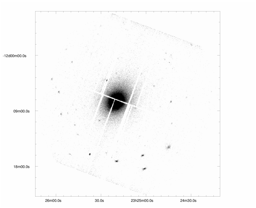
Figure 2: pn count image of Abell 2597, selected with FLAG == 0 && PATTERN $\leqslant$ 4 && PI in [200:15000]. The image has been GTI filtered and corrected for OOT events as described in Section 2, but no vignetting or background correction has been applied. Image pixels are 4$\mathrm{\,arcsec}$ across, roughly the size of the PSF core.

The pn image of the cluster is shown in Fig. 2. As in the ROSAT observation of Sarazin & McNamara (1997), there are a number of non-ICM sources in the field of view, though only two of these are within 6$\mathrm{\,arcmin}$ of the cluster centre. The cluster emission itself displays a relaxed, somewhat elliptical form.

In order to examine the global spectral properties of the cluster, and to check the agreement between the three EPIC detectors, we extracted spectra from an annulus of radius 1–4$\mathrm{\,arcmin}$ centred on the cluster emission peak (J2000: RA = 23h25m19.8s, Dec = -12d07m26s; sky coordinates: $X$ = 23720.5, $Y$ = 23720.5). This radial range was selected to excise any cooling flow region and so that the background contribution was insignificant, in order to have the most simple spectral shape possible. The results of basic single temperature fits are presented in Table 1.

Table 1: Global (1–4$\mathrm{\,arcmin}$) spectral properties.

		A	B	C
	$N_{\mathrm{H}}$	2.49	$1.47_{-0.3}^{+0.3}$	2.49
	$kT$	$3.55_{-0.05}^{+0.05}$	$3.69_{-0.07}^{+0.07}$	$3.55_{-0.05}^{+0.05}$
M1	Z	$0.25_{-0.02}^{+0.02}$	$0.26_{-0.02}^{+0.02}$	$0.26_{-0.03}^{+0.02}$
	z	0.0822	0.0822	$0.078_{-0.002}^{+0.001}$
	$\chi^{2}$	$349.6/343$	$340.5/342$	$342.1/342$
	$N_{\mathrm{H}}$	2.49	$1.91_{-0.3}^{+0.3}$	2.49
	$kT$	$3.43_{-0.05}^{+0.05}$	$3.50_{-0.07}^{+0.07}$	$3.42_{-0.05}^{+0.08}$
M2	Z	$0.22_{-0.02}^{+0.02}$	$0.23_{-0.02}^{+0.02}$	$0.22_{-0.02}^{+0.02}$
	z	0.0822	0.0822	$0.081_{-0.002}^{+0.002}$
	$\chi^{2}$	$297.3/348$	$294.2/347$	$296.8/347$
	$N_{\mathrm{H}}$	2.49	$0.01_{-0.01}^{+0.2}$	2.49
	$kT$	$3.24_{-0.003}^{+0.030}$	$3.59_{-0.04}^{+0.04}$	$3.22_{-0.03}^{+0.02}$
pn	Z	$0.20_{-0.01}^{+0.01}$	$0.25_{-0.01}^{+0.01}$	$0.22_{-0.01}^{+0.01}$
	z	0.0822	0.0822	$0.077_{-0.001}^{+0.0004}$
	$\chi^{2}$	$1321.2/1003$	$1118.8/1002$	$1293.6/1002$
	$N_{\mathrm{H}}$	2.49	$0.59_{-0.1}^{+0.1}$	2.49
	$kT$	$3.35_{-0.005}^{+0.01}$	$3.61_{-0.03}^{+0.03}$	$3.33_{-0.02}^{+0.02}$
All	Z	$0.212_{-0.006}^{+0.003}$	$0.25_{-0.01}^{+0.01}$	$0.23_{-0.01}^{+0.01}$
	z	0.0822	0.0822	$0.079_{-0.001}^{+0.001}$
	$\chi^{2}$	$2000.6/1698$	$1815.8/1697$	$1968.0/1697$

$N_{\mathrm{H}}$ is Galactic column in units of $10^{20}\mathrm{\,cm^{-2}}$; $kT$ temperature in keV; Z metallicity relative to solar. Errors are $1\sigma$. Quantities without errors were fixed. Models A–C are phabs$\times$ mekal, with: Galactic $N_{\mathrm{H}}$; free $N_{\mathrm{H}}$; free $z$. When fitting all three detectors simultaneously, the normalizations were untied (though the effects of this were slight in this instance).

When a fixed, Galactic absorption is used (model A), the pn has a temperature somewhat below that of the MOS instruments, and a higher reduced $\chi^{2}$. If the absorbing column is allowed to vary (model B), then all three detectors prefer a value significantly below Galactic, with the pn $N_{\mathrm{H}}$ being much lower than that of either MOS. Importantly, however, freeing $N_{\mathrm{H}}$ results in the MOS and pn $T$ and $Z$ values coming in to much closer agreement with each other. The conclusion we may draw from this is that all three detectors exhibit some form of soft excess (whose origin is unclear) with respect to a Galactic absorbing column, more so in the pn; but that when the absorbing column is allowed to be free, the three detectors agree reasonably well with regards to the other cluster properties. When all three detectors are analysed simultaneously, the fits adopt a compromise between the pn and MOS values (there are roughly equal numbers of counts in the pn and two MOS combined).

Model C has a fixed $N_{\mathrm{H}}$, but freely varying redshift $z$. The three detectors adopt disparate redshifts, with MOS1 and the pn disagreeing (at the 1$\sigma$ level) with the nominal optical redshift, 0.0822. Analysis of the RGS data, however, with its higher spectral resolution (see Section 5.2), results in a redshift consistent with the optical value. Comparing the results of models A and C (which differ only by whether redshift is free or not), we see that the only effects of freeing $z$ are to reduce $\chi^{2}$ somewhat – the results for other parameters such as $T$ and $Z$ are unchanged. Accordingly, we have left $z$ fixed at the optical value in all subsequent EPIC fits.

Table 2: Global (0–4$\mathrm{\,arcmin}$) spectral properties.

		A	B	D	E	F	G
	$N_{\mathrm{H}}$	2.49	$1.49_{-0.2}^{+0.2}$	2.49	$2.52_{-0.4}^{+0.4}$	2.49	$2.11_{-0.3}^{+0.3}$
	$kT$	$3.35_{-0.03}^{+0.03}$	$3.47_{-0.04}^{+0.04}$	$3.46_{-0.03}^{+0.04}$	$3.45_{-0.03}^{+0.04}$	$3.56_{-0.05}^{+0.05}$	$3.56_{-0.05}^{+0.05}$
	$kT_{2}$	-	-	$0.47_{-0.07}^{+0.07}$	$0.46_{-0.08}^{+0.08}$	-	-
M1	$K_{2}/K$	-	-	$0.015_{-0.002}^{+0.002}$	$0.015_{-0.005}^{+0.005}$	-	-
	$\dot{M}$	-	-	-	-	$93_{-15}^{+15}$	$73_{-19}^{+20}$
	Z	$0.35_{-0.01}^{+0.02}$	$0.37_{-0.02}^{+0.02}$	$0.39_{-0.01}^{+0.01}$	$0.39_{-0.02}^{+0.02}$	$0.37_{-0.02}^{+0.02}$	$0.37_{-0.02}^{+0.02}$
	$\chi^{2}$	$474.9/396$	$450.0/395$	$432.0/394$	$432.1/393$	$437.4/395$	$435.4/394$
	$N_{\mathrm{H}}$	2.49	$1.78_{-0.2}^{+0.2}$	2.49	$2.13_{-0.3}^{+0.3}$	2.49	$2.56_{-0.3}^{+0.3}$
	$kT$	$3.22_{-0.03}^{+0.03}$	$3.30_{-0.03}^{+0.03}$	$3.32_{-0.03}^{+0.03}$	$3.35_{-0.04}^{+0.05}$	$3.40_{-0.04}^{+0.05}$	$3.40_{-0.04}^{+0.05}$
	$kT_{2}$	-	-	$0.75_{-0.09}^{+0.1}$	$0.86_{-0.1}^{+0.2}$	-	-
M2	$K_{2}/K$	-	-	$0.016_{-0.003}^{+0.003}$	$0.015_{-0.006}^{+0.006}$	-	-
	$\dot{M}$	-	-	-	-	$92_{-16}^{+16}$	$96_{-22}^{+22}$
	Z	$0.30_{-0.01}^{+0.01}$	$0.31_{-0.01}^{+0.01}$	$0.32_{-0.02}^{+0.02}$	$0.32_{-0.02}^{+0.02}$	$0.31_{-0.01}^{+0.01}$	$0.31_{-0.01}^{+0.01}$
	$\chi^{2}$	$404.3/400$	$391.9/399$	$375.5/398$	$374.0/397$	$372.0/399$	$371.9/398$
	$N_{\mathrm{H}}$	2.49	$0.47_{-0.1}^{+0.1}$	2.49	$0.87_{-0.1}^{+0.1}$	2.49	$1.11_{-0.1}^{+0.1}$
	$kT$	$3.04_{-0.02}^{+0.02}$	$3.29_{-0.02}^{+0.02}$	$3.20_{-0.02}^{+0.02}$	$2.29_{-0.08}^{+0.08}$	$3.43_{-0.04}^{+0.03}$	$3.43_{-0.03}^{+0.03}$
	$kT_{2}$	-	-	$0.31_{-0.02}^{+0.02}$	$6.78_{-0.6}^{+0.5}$	-	-
pn	$K_{2}/K$	-	-	$0.035_{-0.003}^{+0.003}$	$0.51_{-0.07}^{+0.07}$	-	-
	$\dot{M}$	-	-	-	-	$159_{-10}^{+8}$	$86_{-11}^{+11}$
	Z	$0.278_{-0.008}^{+0.008}$	$0.318_{-0.009}^{+0.009}$	$0.325_{-0.006}^{+0.01}$	$0.27_{-0.01}^{+0.01}$	$0.301_{-0.009}^{+0.009}$	$0.322_{-0.009}^{+0.01}$
	$\chi^{2}$	$1781.8/1190$	$1482.2/1189$	$1537.3/1188$	$1307.4/1187$	$1504.2/1189$	$1417.2/1188$

Models: A, B $\texttt{phabs}{}\times\texttt{mekal}$; D, E $\texttt{phabs}{}\times(\texttt{mekal}+\texttt{mekal})$; F, G $\texttt{phabs}{}\times(\texttt{mekal}+\texttt{mkcflow})$. The first, second model in each pair have Galactic, free $N_{\mathrm{H}}$ respectively. $K_{2}/K$ relative normalization of second temperature component; $\dot{M}$ mass deposition rate ($\mathrm{\,\mathrm{\,M_{\odot}}}$$\mathrm{\,yr^{-1}}$); $Z$ metallicity (solar units).

In Table 2 are shown the results of fitting the entire central 4$\mathrm{\,arcmin}$. Now that we include the cooling region, a wider variety of spectral models become relevant. Models A and B are the same as in the 1–4$\mathrm{\,\arcmin}$ case. The fits in the 0–4$\mathrm{\,arcmin}$ region adopt lower temperatures and higher abundances, so that we may expect to see temperature and abundance profiles that decrease and increase respectively with decreasing radius (see Section 4).

The results of model B can be compared directly with those of Allen et al. (2001), who found, using ASCA: $T=3.38_{-0.07}^{+0.06}$, $Z=0.35_{-0.04}^{+0.03}$, and $N_{\mathrm{H}}=0.99_{-0.08}^{+0.07}$ (90 per cent confidence limits).

In models D and E we add a second mekal component, with an independent temperature and normalization. For all three detectors, the fits are significantly improved. For example, for MOS1 with a free $N_{\mathrm{H}}$, the change in fit statistic is $\Delta\chi^{2}=-17.9$ for the removal of two degrees of freedom. According to the F-test, the significance of such an improvement is ($1-3.4\times 10^{-4}$). Adhering to strict mathematical formalism, the F-test is not really valid in cases such as this (testing for the presence of a second component), where one of the hypotheses lies on the boundary of the parameter space (Protassov et al., 2002). In practice, however, Monte Carlo simulations show that it gives acceptable answers (Johnstone et al., 2002).

The relative normalization of the second temperature component is a few per cent of that of the bulk hot gas. If the hot and cold phases are in pressure equilibrium, then $n_{\mathrm{C}}T_{\mathrm{C}}=n_{\mathrm{H}}T_{\mathrm{H}}$. The normalization of the mekal model varies as $K\propto n^{2}V$. Hence, the relative filling factor of the cold phase is given by

$$V_{\mathrm{C}}/V_{\mathrm{H}}=(K_{\mathrm{C}}/K_{\mathrm{H}})*(n_{\mathrm{H}}/n_{\mathrm{C}})^{2}=(K_{\mathrm{C}}/K_{\mathrm{H}})*(T_{\mathrm{C}}/T_{\mathrm{H}})^{2};$$

which applied to the results in Table 2 for each detector gives values $\sim$ few $\times$ $10^{-4}$ in this case.

Interestingly, when a second temperature component is available, then the fitted $N_{\mathrm{H}}$ for the MOS detectors becomes consistent with the Galactic value. The pn results, however, for model E are not sensibly constrained. It is noticeable that the best-fitting low-temperature components for the two MOS detectors in models D and E are somewhat discrepant. If (as we will argue later on) there really is a cooling flow operating down to low temperatures in this system, then there will be gas present at a continuous range of temperatures, and it is not obvious what the preferred single low-temperature value will be in a model with only two temperature components, nor how it will vary between different instruments. The upper temperatures for the two MOS instruments also seem to be systematically different, albeit at a lower level than for the low temperatures. In terms of the fit, the higher value for $T_{\mathrm{2}}$ in MOS2 seems to be due to a slightly broader iron L hump at 1$\mathrm{\,keV}$ in this detector.

For completeness, we note that the pn results are stable against alternative forms of light-curve filtering and background correction. For example, if we apply the same count-rate cut (0.45$\mathrm{\,ct}$$\mathrm{\,s^{-1}}$) as used in the blank-sky fields of Lumb (2002), and then employ a double background subtraction technique (as used for the MOS), then the pn fits are essentially unchanged.

Using a cooling flow model (in which gas cools from the temperature of the bulk hot gas), instead of a single temperature, for the second component, also provides a significant improvement in fit over a one-component model. The data are not able to distinguish between these two possibilities with any degree of accuracy. For example, for MOS1 a cooling flow provides a very slightly worse fit than a single temperature, whereas for the MOS2 the situation is reversed. The cooling flow fit does have only one extra free parameter though. When the absorbing column is allowed to be free, all three detectors independently fit a mass deposition rate $\sim$ 90$\mathrm{\,\mathrm{\,M_{\odot}}}$$\mathrm{\,yr^{-1}}$. An analysis of the Reflection Grating Spectrometer (RGS) data (Section 5) produces very similar mass deposition results.

In Fig. 3 we show the results of allowing the minimum temperature of the cooling flow component, $T_{\mathrm{min}}$, to vary freely; for both fixed and free $N_{\mathrm{H}}$ (i.e. models F and G in Table 2 respectively). When $T_{\mathrm{min}}$ is allowed to vary freely, a value somewhat above ‘zero’ (i.e. the model minimum, 0.081$\mathrm{\,keV}$) is preferred; but a zero cut-off temperature is entirely consistent with the data, within the 1$\sigma$ limits. The associated mass-deposition rate, $\dot{M}$, is little changed. Freeing $N_{\mathrm{H}}$ broadens the allowed confidence regions, but does not greatly affect the results.

Figure 3: Confidence contours in the $\dot{M}$–$T_{\mathrm{min}}$ plane for the MOS1 + MOS2 cooling flow fits (models F and G in Table 2, but with $T_{\mathrm{min}}$ free to vary). Upper panel fixed $N_{\mathrm{H}}$, lower panel free $N_{\mathrm{H}}$. The cross shows the best-fit value, and the contours are plotted for $\Delta\chi^{2}$ = 2.3, 4.61, 9.21; corresponding to the 68, 90, and 99 per cent confidence limits respectively on two free parameters. The left-hand boundary is due to the lowest usable model temperature, 0.081$\mathrm{\,keV}$.

3.1 Comparison with Chandra

We present a brief comparison of the results of XMM-Newton and Chandra observations of Abell 2597 through a re-analysis of the Chandra observation of McNamara et al. (2001). We use a conservative flare screening of the Chandra data that results in 7$\mathrm{\,ks}$ of good time. The agreement between the Chandra and XMM-Newton pointings for the location of the X-ray emission peak is excellent. The largest complete circle centred on this point that can be extracted from the ACIS-S3 chip has a radius of 1$\mathrm{\,arcmin}$. This encompasses most of the cooling region (see Section 4.2). A background spectrum was extracted from the appropriate standard blank-sky field. The spectrum was fitted over the 0.6–7.0$\mathrm{\,keV}$ range.

Figure 4: Confidence contours in the $\dot{M}$–$T_{\mathrm{min}}$ plane for the central 1$\mathrm{\,arcmin}$ in radius (the cooling region) from the Chandra ACIS-S3 data, with a Galactic $N_{\mathrm{H}}$. Plot details are as per Fig 3.

Fig. 4 is the Chandra counterpart of the upper panel (i.e. for a fixed $N_{\mathrm{H}}$) of Fig. 3 for the MOS. We were unable to obtain sensible constraints when the absorbing column was allowed to vary freely. The preferred low-temperature cut-off for the cooling flow component, though not tightly constrained, is as low as possible. The associated mass deposition rate is $\sim$ 70$\mathrm{\,\mathrm{\,M_{\odot}}}$$\mathrm{\,yr^{-1}}$, entirely consistent with the XMM-Newton EPIC results for the central 4$\mathrm{\,arcmin}$. These results are also in agreement with those from the RGS, as shown in Fig. 17. Fig 4 may be contrasted with the more common Chandra result in such cases, where a much higher $T_{\mathrm{min}}$ is preferred (e.g. in Abell 3581; Johnstone et al., 2005, fig. 10).

4 Radial properties

Given the symmetric nature of the emission visible in Fig. 2, we have performed analyses using circular annuli centred on the cluster emission peak.

4.1 Surface brightness profile

Fig. 5 shows the surface brightness profile of the central 4$\mathrm{\,arcmin}$ in radius of the cluster in the 0.5–2.0$\mathrm{\,keV}$ band, from the sum of the MOS1 and MOS2 data. The profile was extracted from 1$\mathrm{\,arcsec}$ pixel images and vignetting-corrected exposure maps, using circular annuli centred on the emission peak. A background was subtracted using the appropriate scaled blank-field data sets. The width of each annulus was such that the significance of the background-subtracted counts it contained was at least $5\sigma$. Point sources were excluded.

Also shown is the result of a $\beta$ profile fit to the surface brightness, $\Sigma(r)=\Sigma_{0}[1+(r/r_{\mathrm{c}})^{2}]^{-3\beta+0.5}$; with $\beta=0.585_{-0.001}^{+0.002}$, $r_{\mathrm{c}}=23.0_{-0.02}^{+0.02}\mathrm{\,arcsec}$.

The surface brightness profile is affected by the XMM-Newton PSF, which can itself be well described by a $\beta$ model (Ghizzardi, 2001, 2002), with a core radius of around 5$\mathrm{\,arcsec}$. When an intrinsic brightness profile $a(\vec{r})$ is modified by an instrumental PSF $b(\vec{r})$, the observed profile is the convolution of the two,

$$c(\vec{r})=\int\,\mathrm{d}^{2}\vec{u}\;a(\vec{u})b(\vec{r}-\vec{u})=2\pi\int_{0}^{\infty}\,\mathrm{d}k\;kJ_{0}(kr)\tilde{a}(k)\tilde{b}(k),$$ (1)

where the second form is for the case of radial symmetry and makes use of the convolution theorem. $\tilde{a}(k)$ in this expression is the radially symmetric Fourier transform (Birkinshaw, 1994), or Hankel transform of order zero,

$$\tilde{f}(k)=\int_{0}^{\infty}\,\mathrm{d}r\;J_{0}(kr)rf(r),$$ (2)

with $J_{0}$ a Bessel function of the first kind. Evaluating the effect of instrument PSF on a surface brightness profile therefore reduces to performing three Hankel transforms. The general $\beta$ function has an analytic Hankel transform (Gradshteyn & Ryzhik, 2000, equation 6.565.4), but the specific case of $\beta=2/3$, which is a good approximation for both the XMM-Newton PSF and many cluster brightness profiles, is especially simple:

$$f(r)=(a^{2}+r^{2})^{-3/2} \Leftrightarrow \tilde{f}(k)=\frac{\mathrm{e}^{-ak}}{a}$$ (3)

As a result, if

$$S(r)=S_{0}[1+(r/r_{\mathrm{s}})^{2}]^{-3/2} \mathrm{and} P(r)=P_{0}[1+(r/r_{\mathrm{p}})^{2}]^{-3/2}$$ (4)

describe the source and PSF profiles respectively, with the latter normalized so that $P_{0}=(2\pi r_{\mathrm{p}})^{-1}$, then it is straightforward to show that the convolution $c(r)$ is given by

$$c(r)=S_{0}\Big{(}\frac{r_{\mathrm{s}}}{r_{\mathrm{s}}+r_{\mathrm{p}}}\Big{)}^{2}\left[1+\Big{(}\frac{r}{r_{\mathrm{s}}+r_{\mathrm{p}}}\Big{)}^{2}\right]^{-3/2}.$$ (5)

This is nothing more than another $\beta$ profile, with a reduced central amplitude $S^{\prime}_{0}$ and increased core radius $r^{\prime}_{\mathrm{s}}$:

$$S^{\prime}_{0}=S_{0}\Big{(}1+\frac{r_{\mathrm{p}}}{r_{\mathrm{s}}}\Big{)}^{-2}\sim S_{0}\Big{(}1-2\frac{r_{\mathrm{p}}}{r_{\mathrm{s}}}\Big{)} \mathrm{and} r^{\prime}_{\mathrm{s}}=r_{\mathrm{s}}+r_{\mathrm{p}}.$$ (6)

The simplest PSF correction we can make to the surface brightness profile is therefore to subtract the radius of the PSF, 5$\mathrm{\,arcsec}$, from the core fitted to the convolved profile, 23$\mathrm{\,arcsec}$, resulting in an estimate of 18$\mathrm{\,arcsec}$ for the intrinsic surface brightness core radius.

Figure 5: Surface brightness profile of the central 240$\mathrm{\,arcsec}$ in radius, 0.5–2.0$\mathrm{\,keV}$ band, from summed MOS1 and MOS2 profiles. The dotted line shows a $\beta$ profile fit to the data – see text for details. The profile has been corrected for background and vignetting.

4.2 Spectral profiles

In order to obtain reliable spectral fits, annular radii were chosen so as to encompass slightly more than 10000 (net, i.e. background-subtracted) counts in each MOS, and thus over 20000 counts in the pn. It was found that annuli with fewer counts (e.g. 7500 per MOS) tended to give poor (unphysical) results in the deprojection and PSF-correction analyses. In such cases, the lower signal-to-noise allows physically unrealistic solutions (in which fitted quantities tend to oscillate about the smoother profiles obtained from annuli with more counts) to become mathematically valid. Both correction algorithms (see e.g. Johnstone et al. 2005 for testing of the deprojection process) involve redistribution of counts between annuli, potentially (depending on the details of the brightness profile) leaving small net numbers of counts in any one annulus. In practice it is found to be beneficial not to let the uncorrected count numbers fall too low. The outermost annulus was truncated at a radius of 5$\mathrm{\,arcmin}$ (due to the increasing relative background) and so contains somewhat fewer counts. By the time this last annulus is reached, the background is contributing about 30 per cent of the total counts.

4.2.1 Projected profiles

Fig. 6 shows the results of fitting a single-temperature mekal (Mewe et al., 1995) model to each spectral annulus, with an uniform (but free to vary) absorbing column applied to all annuli. The central temperature is a little over 2.5$\mathrm{\,keV}$ (a function of the size of the central annulus). Over the central 100$\mathrm{\,kpc}$ or so the temperature increases, reaching a maximum of $\sim 3.6$$\mathrm{\,keV}$. Outside the central cooling region, there is perhaps evidence for a gradual decline in temperature beyond $\sim 150$$\mathrm{\,kpc}$ or so. The metallicity exhibits a fairly smooth decline with increasing radius in the central cooling region, dropping from around 0.5$\mathrm{\,\mathrm{\,Z_{\odot}}}$ at the centre to 0.2$\mathrm{\,\mathrm{\,Z_{\odot}}}$ at the outside.

Results are shown for the simultaneous fit of both MOS instruments, and also for the pn. The two instruments agree reasonably well in terms of $T$ and $Z$, but have very different preferences for $N_{\mathrm{H}}$.

Figure 6: Projected temperature (upper panel) and metallicity (lower panel) profiles. The open triangles are simultaneous MOS1 + MOS2 fits, the filled squares are the pn. The model was $\texttt{phabs}\times\texttt{mekal}$ with a common, free absorbing column $N_{\mathrm{H}}$ shared by all annuli. The $N_{\mathrm{H}}$ values were (in units of $10^{20}$$\mathrm{\,cm^{-2}}$): $1.52_{-0.08}^{+0.08}$ (MOS); $0.19_{-0.06}^{+0.06}$ (pn). With $N_{\mathrm{H}}$ free to vary between annuli, the T and Z profiles are not much changed. The MOS $N_{\mathrm{H}}$ shows no significant variation with radius; whereas that of the pn is consistent with the MOS in the central two bins, but much lower outside this region.

In Fig. 7, we show the radial dependence of the cumulative mass deposition rate, $\dot{M}(<r)$, within the cooling flow radius (130$\mathrm{\,kpc}$; see Section 4.2.2). There is a discrepancy between the MOS and pn detectors, with the former preferring smaller mass deposition rates. Owing to the way this figure was constructed (fitting each annulus independently with a single temperature component and a cooling flow component, then summing the $\dot{M}$ values so obtained from the centre outwards), the discrepancy between the two instruments builds with increasing radius. Also shown is the $\dot{M}$ value inferred by Oegerle et al. (2001) from their FUSE data; namely 40$\mathrm{\,\mathrm{\,M_{\odot}}}$$\mathrm{\,yr^{-1}}$ within a radius of 40$\mathrm{\,kpc}$. The figure illustrates that there is reasonable agreement between the X-ray and UV mass deposition rates within a radius of 40$\mathrm{\,kpc}$.

Figure 7: Cumulative projected mass deposition rate, $\dot{M}(<r)$, for the cooling flow region. The open triangles are simultaneous MOS1 + MOS2 fits, the filled squares are the pn. The model was $\texttt{phabs}\times(\texttt{mekal}+\texttt{mkcflow}$) with a fixed Galactic absorption. The star shows the FUSE O 6 data point of Oegerle et al. (2001), with an error bar appropriate for the accuracy of the FUSE flux measurement, $(1.3\pm 0.35)\times 10^{-15}\mathrm{\,erg}\mathrm{\,cm^{-2}}\mathrm{\,s^{-1}}$.

4.2.2 Deprojected profiles

The results of Fig. 6 are subject to projection effects, in which the spectral properties at any point in the cluster are the emission-weighted superposition of radiation originating at all points along the line of sight through the cluster. In Fig. 8 we show the results of a deprojection of the MOS and pn spectra using the xspec projct model. Under the assumption of intrinsic spherical (more generally, ellipsoidal) shells of emission, this model calculates the geometric weighting factors according to which emission is redistributed amongst the projected annuli.

Figure 8: Deprojected temperature (upper panel) and metallicity (lower panel) profiles. The open triangles are simultaneous MOS1 + MOS2 fits, the filled squares are the pn (as per Fig. 6). The model was $\texttt{projct}\times\texttt{phabs}\times\texttt{mekal}$ with a common, free absorbing column $N_{\mathrm{H}}$ shared by all annuli. The $N_{\mathrm{H}}$ values were (in units of $10^{20}$$\mathrm{\,cm^{-2}}$): $1.53_{-0.08}^{+0.08}$ (MOS); $0.23_{-0.06}^{+0.06}$ (pn); little changed from the projected results.

As is to be expected, the temperature in the outer regions where the profile is fairly flat is seen to be relatively little influenced by projection. Deprojection recovers a lower central temperature than before, since in the projected fits the spectrum of the central annulus is contaminated by overlying hotter emission. There is also some evidence for a higher central abundance in the deprojected metallicity profile.

The deprojected pn temperature profile shows some signs of instability in the centre, in which neighbouring bins ‘oscillate’ with high and low temperatures. The interpolated values, though, agree well with the MOS results. Recently, Johnstone et al. (2005) have shown that the projct approach works well at reproducing various simple synthetic cluster temperature and density structures. Possibly the slight instability of the pn fit reflects a more complex under-lying temperature distribution (e.g. more than one phase); but more likely it is simply a quirk of geometry that renders certain physically unrealistic solutions mathematically plausible. Freezing the abundances at the projected value makes little difference, but the effect can be removed by using larger annuli (although the pn annuli shown already contain similar numbers of counts to the combined MOS annuli), but we retain the same annuli here for both instruments for illustration.

Figure 9: Derived quantities from the deprojected profiles of Fig. 8: upper panel electron density; middle panel approximate isobaric cooling time; lower panel entropy. The dotted lines show the fits of some simple models to the data: a beta profile for the density; and a constant plus power-law for the entropy. See text for details.

In Fig. 9 we show various quantities derived from the deprojected spectral fits. The electron density $n_{\mathrm{e}}$ is obtained from the mekal normalization, and scales as $H_{0}^{1/2}$. The cooling time (scaling as $H_{0}^{-1/2}$) is an approximate isobaric one, calculated as the time taken for the gas to radiate its enthalpy using the instantaneous cooling rate at any temperature,

$$t_{\mathrm{cool}}\approx\frac{H}{n_{\mathrm{e}}n_{\mathrm{H}}\Lambda(T)}=\frac{\gamma}{\gamma-1}\frac{kT}{\mu X_{\mathrm{H}}n_{\mathrm{e}}\Lambda(T)},$$ (7)

where: $\gamma=5/3$ is the adiabatic index; $\mu\approx 0.61$ (for a fully-ionized 0.3$\mathrm{\,\mathrm{\,Z_{\odot}}}$ plasma) is the molecular weight; $X_{\mathrm{H}}\approx 0.71$ is the hydrogen mass fraction; and $\Lambda(T)$ is the cooling function. The ‘entropy’ is the standard astronomer’s entropy, $S=Tn_{\mathrm{e}}^{-2/3}$, and scales as $H_{0}^{-1/3}$.

The cooling time is less than 10$\mathrm{\,Gyr}$ inside a radius of 130$\mathrm{\,kpc}$ (in perfect agreement with the ROSAT result of Sarazin et al. 1995), and less than 5$\mathrm{\,Gyr}$ inside 85$\mathrm{\,kpc}$.

Also shown in Fig. 9 are the results of simple model fits to the density and entropy profiles. The density profile is represented by a $\beta$ model, $n(r)=n_{0}[1+(r/r_{\mathrm{c}})^{2}]^{-1.5\beta}$; with $\beta=0.57_{-0.01}^{+0.01}$, $n_{0}=0.0354_{-0.0006}^{+0.0006}\mathrm{\,cm^{-3}}$, $r_{\mathrm{c}}=49.0_{-0.9}^{+0.9}\mathrm{\,kpc}$. These results for the density profile are in reasonable agreement with those obtained from fitting the surface brightness profile (Section 4.1). The absence of a significant excess in the deprojected density in the last annulus indicates that we reach a sufficiently large radius that projection from more distant material is not significant (compare with the Chandra deprojection results of Johnstone et al., 2005). The entropy profile is parametrized as a constant plus power-law, $S(r)=S_{0}+kr^{\eta}$; with $S_{0}=15.1_{-1.5}^{+1.5}\mathrm{\,keV}\mathrm{\,cm^{2}}$, $k=0.28_{-0.05}^{+0.05}\mathrm{\,keV}\mathrm{\,cm^{2}}\mathrm{\,kpc^{-1.19}}$, $\eta=1.19_{-0.04}^{+0.03}$. The fit with the $S_{0}$ term is substantially better than that without, but bear in mind that the PSF has not been corrected for here. A logarithmic slope for the entropy profile of $\approx 1.1$ is produced in simulations involving gravitational collapse and shock heating (Tozzi & Norman, 2001).

The virial radius becomes a quantity of interest at this point. It is known that the calibrations of the scaling relations obtained from simulations have normalizations quite different to those obtained from observation. Allen et al. (2001) studied the cluster virial scaling relations using Chandra, but do not quote an explicit radius–temperature relation. Using their data for an SCDM cosmology, we calibrate the $r$–$T$ relation as $r_{2500}=0.31\mathrm{\,Mpc}\;h_{50}^{-1}(1+z)^{-3/2}(T_{2500}/\mathrm{\,keV})^{0.5}$. The conversion from an overdensity of 2500 to one of 200 (appropriate for the virial radius) depends upon the form assumed for the density profile. Taking an NFW profile with a typical cluster concentration $c=5$, we find that $r_{200}\approx 2.75r_{2500}$. Using a temperature of 3.5$\mathrm{\,keV}$, we therefore estimate a virial radius of 1.4$\mathrm{\,Mpc}$ for Abell 2597. The radius 0.1$R_{\mathrm{V}}$ therefore lies within the sixth annulus from the centre (a bin whose mid-point is at 150$\mathrm{\,kpc}$). The measured entropy in this bin is $S_{0.1R_{\mathrm{V}}}=(137\pm 6)h_{50}^{-1/3}$$\mathrm{\,keV}$$\mathrm{\,cm^{2}}$. This is a relatively low value (see e.g. fig. 4 of Ponman et al., 2003), but recall PSF effects are still present in this result.

4.2.3 PSF-corrected profiles

The broadening effect of the XMM-Newton PSF acts to redistribute counts between spectral annuli in a manner conceptually similar to that of projection. Consequently, it can be corrected for in the same way, namely by using an xspec mixing model, xmmpsf.

The most recent version available at the time of writing was unable to fit observations from different instruments simultaneously, so we present here only the results for MOS1, in order to illustrate the effects of PSF on the spectral fits. We have been unable to achieve physically realistic solutions when using the xmmpsf and projct models in combination, to correct for both projection and PSF at the same time. The exception is when annuli that are physically very large are employed; but in such cases the PSF redistribution becomes less significant anyway, and we also obtain very limited resolution of the central cooling region, which is the main area of interest here.

For a given set of spectral annuli, and a given brightness profile, the xmmpsf model calculates the mixing factors through which flux from any given annulus is redistributed to all the others. The factors are calculated at ten energies in the range 0.5–6.0$\mathrm{\,keV}$, although the energy dependence of the XMM-Newton PSF is relatively small. The input brightness profile can be specified using either an image, or a model parametrization. We find that there is no significant difference between using a MOS1 (say) image or the PSF-corrected $\beta$ profile from Section 4.1 to provide the brightness information. By way of example, we show the mixing factors for our set of annuli at 1.0$\mathrm{\,keV}$ in Fig. 10. At the ten per cent level, each annulus is only affected by its immediate neighbours. Nevertheless, the mixing is potentially quite significant, since for many regions only 50 per cent of their flux originates from that same region.

Figure 10: xmmpsf mixing factors calculated at 1.0$\mathrm{\,keV}$. Each curve shows, for one of the annular regions, the fraction of the flux in that region originating from each of the other regions. Only contributions greater than 1 per cent are shown. The peak flux is always from the region itself. The actual mixing factors used internally by the model relate to the fraction of the flux from each region going to other regions. The factors shown here are calculated from these using the model normalizations fitted to each annulus. By construction, the points with the same x-coordinate sum to 1.0.

In Fig. 11, we show the $T$ and $Z$ profiles obtained from a PSF-corrected fit of the MOS1 data. Compared to the uncorrected profiles (Fig. 6), a steeper central temperature gradient is recovered, as well as a larger central abundance peak.

Figure 11: PSF-corrected MOS1 temperature (upper panel) and metallicity (lower panel) profiles. The model was $\texttt{xmmpsf}\times\texttt{phabs}\times\texttt{mekal}$ with a common, free absorbing column shared by all annuli: $N_{\mathrm{H}}=1.40_{-0.1}^{+0.1}10^{20}\mathrm{\,cm^{-2}}$.

Fig. 12 displays the density, cooling time, and entropy derived from the PSF-corrected profiles. Compared to the results of Fig. 9, a higher central density, and a lower central cooling time and entropy are obtained. Also shown is a $\beta$ model fit for the density, with: $\beta=0.579_{-0.004}^{+0.004}$, $n_{0}=0.068_{-0.001}^{+0.001}\mathrm{\,cm^{-3}}$, $r_{\mathrm{c}}=31.6_{-0.6}^{+0.6}\mathrm{\,kpc}$. The PSF corrected core radius of 15$\mathrm{\,arcsec}$ is comparable to the estimate of 18$\mathrm{\,arcsec}$ made in Section 4.1 using the surface brightness profile.

The entropy profile is well-fit – reduced $\chi^{2}=7.49/(9~{}-~{}3)$ – by a constant plus power-law model of the same form used in Section 4.2.2, with: $S_{0}=7.9_{-1.5}^{+1.3}\mathrm{\,keV}\mathrm{\,cm^{2}}$, $k=0.40_{-0.08}^{+0.11}\mathrm{\,keV}\mathrm{\,cm^{2}}\mathrm{\,kpc^{-1.15}}$, $\eta=1.15_{-0.04}^{+0.05}$.

Figure 12: Derived quantities from the MOS1 PSF-corrected profiles of Fig. 11. Details as per Fig. 9.

4.3 Comparison with Chandra temperature profile

As per Section 3.1, we have compared the XMM-Newton and Chandra results. Chandra spectra were extracted from the same annuli as used in the XMM-Newton analysis. Restricting ourselves to those annuli that lie entirely on the ACIS-S3 chip, we obtain five spectral regions from the Chandra data. Background spectra were produced as previously described (though background should not be significant in this region).

In Fig. 13 we compare the temperature profiles obtained from MOS1 and Chandra, using a simple $\texttt{phabs}\times\texttt{mekal}$ model with a fixed Galactic absorption. The agreement between the MOS1 and ACIS temperatures is good everywhere except in the central bin, where the ACIS temperature is significantly lower than that of the MOS. Correcting for the XMM-Newton PSF using the xmmpsf model in the previously described manner lowers the central MOS1 temperature so that it agrees very well with that of Chandra. The agreement of the other MOS1 points with those of ACIS is worsened though, as the PSF correction raises all but the central MOS1 temperatures.

The XMM-Newton/Chandra cross-calibration has recently been examined by Kirsch et al. (2004).

Figure 13: Comparison of MOS1 and Chandra ACIS-S3 temperature profiles. Open symbols MOS1: circles non-PSF corrected; stars PSF corrected. Filled squares Chandra. The model in each case was $\texttt{phabs}\times\texttt{mekal}$ with a fixed Galactic $N_{\mathrm{H}}$. The PSF correction was achieved with the addition of an xmmpsf component (see text for details).

5 Reflection Grating Spectrometer

Around half of the light in each telescope feeding the MOS detectors is diverted to a Reflection Grating Spectrometer (RGS; den Herder et al., 2001). Each RGS contains 9 CCDs (though one has failed in each RGS) along the dispersion direction, and is sensitive to soft X-rays in the range $\sim$ 6–38 Å. The field of view in the cross-dispersion direction is 5$\mathrm{\,arcmin}$.

5.1 Data reduction

The two RGS were operated in the standard Spectroscopy mode. Data were processed from the ODFs using the SAS meta-task rgsproc. The position of the cluster emission peak as measured from the MOS image was used to specify the source extraction point. The generated RGS1 and RGS2 events files were filtered for periods of high background with the same approach as used in the construction of the RGS background files (Tamura et al., 2003). Indeed, since the background files do not have the necessary information for further filtering, we have little choice but to proceed in this manner (though we might prefer to use a stricter filtering in this case). That is, we form a light-curve from the (FLAG == 8,16) events at high cross-dispersion angles ($|$XDSP_CORR$|>$ 1.5e-4) on CCD9 (that which covers the highest energy band and is most affected by background), using 100 second time bins. Only periods with count-rates less than 0.15 counts per second for each RGS were retained, leaving $\sim$ 74$\mathrm{\,ks}$ of time per RGS. Observe that although this is significantly larger than the remaining EPIC exposure, both EPIC and RGS have (essentially) been filtered to the same level as the appropriate ESA-supplied background templates (soft protons channelled through the mirrors are responsible for most of the XMM-Newton background flaring, and relatively few are scattered by the gratings into the RGS detectors).

Since the field of view in the cross-dispersion direction is only 5$\mathrm{\,arcmin}$ wide, it is essentially filled by cluster emission from Abell 2597. We therefore make use of the standard background template files provided by Tamura et al. (2003). We note that these files were made at an operating temperature of -80^∘C, but that in late 2002 both RGS were cooled to -110^∘C.

Figure 14: Profile of RGS1 counts in 10$\mathrm{\,arcsec}$ bins in the cross-dispersion direction, for the events lying in the first order PI-$\beta$ (dispersion angle) selection region.

In Fig. 14 we show the ‘one-dimensional surface brightness’ profile obtained from RGS1 by summing counts in 10$\mathrm{\,arcsec}$ bins in the cross-dispersion direction. The centre of Abell 2597 is unfortunately offset from the mid-point of the CCD array by about 1$\mathrm{\,arcmin}$. There are insufficient counts to form profiles in narrow energy bands, in order to examine the possible differences between the profiles of different spectral lines, e.g. due to resonant scattering (Sakelliou et al., 2002).

RGS spectra are extracted by making selections both in the spatial (dispersion/cross-dispersion) and energy (dispersion/PI) planes, by making use of the intrinsic energy discrimination of the detector CCDs. Due to the extended nature of the source, we have used slightly broader selection criteria than the defaults. Our spatial selection took 97 per cent of the PSF in the cross-dispersion direction, which is equivalent to the central 2$\mathrm{\,arcmin}$ or so of the cluster, i.e. the central cooling region. In the energy plane we took 94 per cent of the pulse-height distribution. We restricted our analysis to the first order spectra.

Response files were generated using the SAS task rgsrmfgen with standard parameters (4000 energy bins between 0.3 and 2.8$\mathrm{\,keV}$). Spectra were grouped to a minimum of 20 counts per bin. RGS source and background spectral channels can have different qualities, and since xspec ignores quality information in the background spectrum, the source PHA files were modified by adding in any extra bad channels from the background spectra. We fit the two RGS instruments simultaneously over the 5–38 Å range, thereby compensating for the missing iron L complex and O 8 line absent (due to failed CCDs) from RGS1 and RGS2 respectively.

In an attempt to deal with the spectral blurring that results from the extended nature of the source, we have employed the xspec rgsxsrc model (due to A. Rasmussen). This convolves the spectral model with an angular structure function computed from an image (we used the MOS1 image in the RGS energy range of 0.3–2.5$\mathrm{\,keV}$) of the target region. Correcting for broadening in this way is only an approximation to the complex instrument response to a spatially extended input. The rgsxsrc model assumes that the spatial structure of the source is independent of energy. To test the possible consequences of this assumption, we examined the effects of using input images in different energy ranges (e.g. below 1$\mathrm{\,keV}$, or dividing the RGS energy range in two and using either the upper or lower half). The results quoted in subsequent sections were found to have very little dependence on the energy range used for the rgsxsrc image. For example, the changes in fitted fluxes for the Fe 17 lines (see Section 5.3) when using a different energy range for the rgsxsrc image are typically of order a few per cent, in a random direction (i.e. not systematically higher or lower for an image in any given energy range). The changes in line significances were negligible.

According to the XMM-Newton Users’ Handbook, the theoretical wavelength resolution of the RGS spectral order $n$ for an extended source of angular size $\theta$ ($\mathrm{\,arcmin}$) is degraded according to the formula $\Delta\lambda/\mathrm{\,\mbox{\AA}}\approx 0.138\;\theta/n$. Thus, for a source region with extent $\sim 2\mathrm{\,arcmin}$ we may expect a wavelength resolution $\approx 0.25\mathrm{\,\mbox{\AA}}$. This is borne out by examination of the model width of an rgsxsrc-blurred line of zero intrinsic width.

5.2 Broad-band spectral fits

In Fig. 15 we show the best-fitting single temperature vmekal model and its $\chi^{2}$ residuals as applied to the data. The abundances of iron and oxygen were allowed to vary independently (both these elements exhibit strong line features in the RGS energy range, so we may reasonably expect to obtain reliable constraints on their individual abundances), whilst those of all the other elements were tied together. The redshift and absorbing hydrogen column were also allowed to vary. Good fits (even with a single temperature model) could not be obtained when the absorption was fixed at Galactic. The fit parameters are listed in Table 3. The preferred absorption is substantially higher than Galactic (and that favoured by the EPIC instruments), for reasons that are not clear. The excess of $N_{\mathrm{H}}$ above Galactic is consistent with the intrinsic $N_{\mathrm{H}}$ (Section 1) detected by O’Dea et al. (1994); but that was only seen against the small central radio source, so this is probably not significant. Allowing $N_{\mathrm{H}}$ to vary results in temperatures and abundances that are consistent with those of the EPIC fits to the similar spatial region.

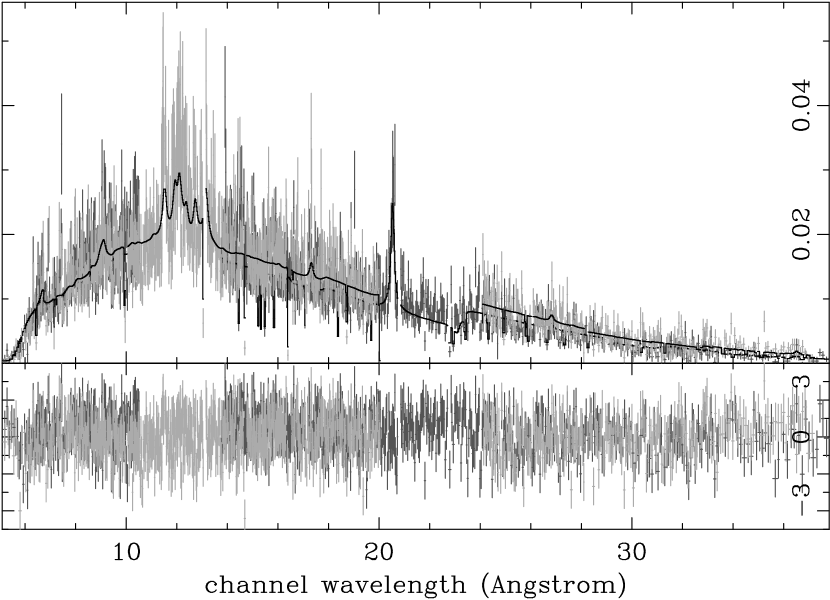
Figure 15: RGS1 (dark) and RGS2 (light) spectra, in units of $\mathrm{\,ct}$$\mathrm{\,\mbox{\AA}^{-1}}$$\mathrm{\,s^{-1}}$. Also shown is the best-fitting single temperature model, together with its $\chi^{2}$ residuals (lower panel).

Table 3: Results of RGS fits to the central $\sim 2$$\mathrm{\,arcmin}$ region, 5–38 Å.

	A	B	C	D
$N_{\mathrm{H}}$	$6.93_{-0.5}^{+0.2}$	$6.19_{-0.3}^{+0.3}$	$6.22_{-0.2}^{+0.2}$	$6.30_{-0.3}^{+0.2}$
$kT$	$2.54_{-0.09}^{+0.16}$	$3.01_{-0.20}^{+0.13}$	$3.12_{-0.13}^{+0.06}$	$3.07_{-0.15}^{+0.22}$
$kT_{2}$	-	$0.66_{-0.03}^{+0.03}$	-	$0.081_{-0}^{+0.13}$
$\dot{M}$	-	-	$95_{-14}^{+14}$	$92_{-11}^{+18}$
$Z_{\mathrm{O}}$	$0.38_{-0.03}^{+0.02}$	$0.44_{-0.05}^{+0.04}$	$0.40_{-0.04}^{+0.04}$	$0.40_{-0.03}^{+0.04}$
$Z_{\mathrm{Fe}}$	$0.22_{-0.02}^{+0.04}$	$0.35_{-0.05}^{+0.02}$	$0.34_{-0.03}^{+0.03}$	$0.33_{-0.02}^{+0.05}$
$Z_{\mathrm{x}}$	$0.28_{-0.06}^{+0.06}$	$0.44_{-0.04}^{+0.07}$	$0.40_{-0.07}^{+0.07}$	$0.39_{-0.07}^{+0.06}$
$z$	$0.0826_{-0.0003}^{+0.0004}$	$0.0826_{-0.0007}^{+0.0001}$	$0.0821_{-0.0002}^{+0.0006}$	$0.0824_{-0.0005}^{+0.0002}$
$\chi^{2}$	$1881.2/1670$	$1852.7/1668$	$1850.8/1669$	$1851.5/1668$

$N_{\mathrm{H}}$ is Galactic column in units of $10^{20}\mathrm{\,cm^{-2}}$; $kT$ temperature in keV; Z metallicity relative to solar for O, Fe, and all other elements (x); and $z$ redshift. Errors are $1\sigma$. All models are rgsxsrc $\times$ phabs $\times$ (M), where M is: A vmekal; B vmekal + vmekal; C vmekal + vmcflow (with vmcflow: $T_{\mathrm{max}}$ $\equiv$ vmekal:$T$, vmcflow:$T_{\mathrm{min}}$ $\equiv$ 0.081); D as C but with $T_{\mathrm{min}}$ free. Where two phases were used, the metallicities were tied.

5.2.1 Redshift issues

Two similar, but distinct, redshifts are in common use for Abell 2597. Kowalski et al. (1983), as used in the compilation of Struble & Rood (1999), measured the optical redshifts of three (non-cD) cluster galaxies as $z=0.0874,0.0832,0.0851$, hence $\bar{z}=0.0852\pm 0.002$ (relative to Local Group standard of rest). Converting this result to heliocentric using the NASA/IPAC Extragalactic Database (NED) velocity converter subtracts $\sim 140\mathrm{\,km}\mathrm{\,s^{-1}}$, giving $z_{\mathrm{helio}}=0.0847$. In contrast, Noonan (1981), using Schmidt (1965), has $z=0.0821$ (heliocentric), based on the central radio galaxy. Owen et al. (1995) find a heliocentric $z=0.0822\pm 0.0002$, using optical emission lines of the central radio galaxy PKS 2322-12. The best-fit redshift found by Voit & Donahue (1997) for the optical emission line nebula in Abell 2597 is $z=0.0821\pm 0.0002$. In light of all this, we choose to adopt $z=0.0822$ for the heliocentric redshift of the cluster.

The best-fitting RGS broad-band redshift is consistent with the adopted optical redshift. The most prominent single line in the spectrum is that of O 8 $\mathrm{K}\alpha$ at around 20.5 Å. The rest energy of this feature is 653.6$\mathrm{\,eV}$. Fitting the spectrum in the 19-22 Å range with an rgsxsrc-blurred power-law plus a (zero intrinsic width) Gaussian, we find the best-fit value for the energy of this line to be $E=603.8_{-0.4}^{+0.2}$$\mathrm{\,eV}$, implying a redshift of $z=0.0825_{-0.0004}^{+0.0007}$, consistent with the broad-band RGS fit, and the optical value.

We have also fit just the iron L complex, by restricting attention to the 9.2–17 Å range (chosen to exclude the Mg line around 9 Å, and to include as much line-free continuum around the Fe L complex as possible). The plasma properties are not well constrained in such a narrow wavelength range, with the exception of redshift, which is our sole interest here. According, we froze $N_{\mathrm{H}}$ at the broad-band value, and fit the data with a single mekal model. The best-fitting redshift for the Fe L complex was $z=0.0831_{-0.0016}^{+0.0002}$. As per Still & Mushotzky (2002), the best-fit O 8 redshift is formally less than that of the Fe L complex. Within the 1$\sigma$ limits, however, the redshifts obtained from the various RGS fits (broad-band, Fe L complex, O 8) are consistent, and agree with our adopted optical redshift. The hypothesis of separate velocity components in the core (Still & Mushotzky, 2002) could therefore be supported by these data, but does not seem to be required.

5.2.2 Additional fit components

Also shown in Table 3 are the results of adding a second temperature component to the fit, with an independent temperature and normalization. The removal of two degrees of freedom results in a change in fit of $\Delta\chi^{2}=-28.5$. According to an F-test, this improvement in fit is significant at the (1 - $3.1\times 10^{-6}$) level. In Fig. 16 we show the contributions made by each of the two temperature components to the total model. The bulk of the spectral fit is obviously dominated by the high-temperature component. The low-temperature component contributes several emission lines at wavelengths around 15 Å – these are examined in more detail below.

Figure 16: Contributions of the two temperature components (solid lines) of model B in Table 3 to the total (dotted line) model. The minority component is the low-temperature one.

In Table 3 we also show the results of fits using a cooling flow (vmcflow model) rather than a single temperature for the second component. These also provide significant improvements to the single-temperature fit, although the data are not of sufficient quality to unambiguously state that a cooling-flow fit is preferred. The most interesting aspect of the fit is the obtained mass deposition rate: $\dot{M}\sim 100$$\mathrm{\,\mathrm{\,M_{\odot}}}$$\mathrm{\,yr^{-1}}$. This is consistent with the EPIC fits to the central regions, Table 2.

Allowing the low-temperature cut-off of the cooling flow component, $T_{\mathrm{min}}$, to be free (rather than fixed at the lowest value possible in the xspec model, 0.081$\mathrm{\,keV}$), makes no improvement to the fit quality. Indeed, as we show in Fig. 17, a very low temperature cut-off for the cooling flow is preferred. The slight upward curve of the significance contours does indicate that higher mass deposition rates are permissible (though not preferred) with higher low-temperature cut-offs.

Figure 17: Confidence contours for the RGS cooling flow fit (model D in Table 3) in the $\dot{M}$–$T_{\mathrm{min}}$ plane. Plot details are as per Fig 3. Compare also with the Chandra results of Fig 4.

5.3 Fe 17 line fitting

We now return to the low-temperature emission lines in the 15 Å region of the spectrum previously alluded to. The Fe 17 lines in this region are particularly important because they are strong indicators of gas at temperatures $\sim$ 0.3$\mathrm{\,keV}$, and consequently their presence is an important prediction of the cooling flow model.

In order to examine these lines in more detail, we fit the 15–20 Å region with a blurred power-law and four (zero intrinsic width) Gaussians. Adopting a fixed redshift of $z=0.0822$, the line energies were fixed at the positions appropriate for the 15.02, 16.78, 17.08 Å (rest wavelength) Fe 17 lines, and the 16.00 Å O 8 $\mathrm{K}\beta$ line. We found the best-fit and $1\sigma$ limits on the normalizations of each line. We obtained positive (but weak) evidence for all three important Fe 17 lines, at the 1–2$\sigma$ level (too low to qualify for a formal detection).

The normalizations were converted to line fluxes (using a luminosity distance of 503$\mathrm{\,Mpc}$) by subtracting off the continuum component in the absence of a line. Results are shown in Table 4.

We have also converted these fluxes to equivalent cooling flow mass deposition rates. This was achieved by using the mkcflow model in xspec to make a fake spectrum for a fiducial 1000$\mathrm{\,\mathrm{\,M_{\odot}}}$$\mathrm{\,yr^{-1}}$ cooling flow, at a redshift etc. appropriate to Abell 2597. We fit the 15–20 Å range of this model spectrum in the same way as applied to the actual data, in order to obtain the flux expected in each of the Fe 17 lines. The ratios of the Abell 2597 line fluxes to those from the model were used to estimate the associated mass-flow rates. The results, as shown in Table 4, are poorly constrained, but consistent with both the broad-band RGS fits, and the EPIC fits to the central region.

Table 4 also gives the F-test significance (the comments of Section 3 on the F-test also apply here) for each of the Fe lines. This is obtained from the improvement in fit that results when fitting a model with just the O 8 and each Fe line in turn present, compared to the best-fit with just the O line. The O line has been treated separately due to its different temperature dependence. The significance of each individual Fe line is admittedly low, varying from about 1–2$\sigma$. In order to try and achieve greater significance, we have tied the relative normalizations of the three Fe 17 lines (all with similar temperature dependences) to that present in the fiducial isobaric cooling flow model, and just allowed the overall normalization to vary. The results are given in the ‘All’ row of Table 4. When combining the lines in this way, the significance is still low, but exceeds $2\sigma$.

Table 4: RGS Fe 17 line fits.

$\lambda/\mathrm{\,\mbox{\AA}}$	Power / $10^{40}$$\mathrm{\,erg}$$\mathrm{\,s^{-1}}$	$\dot{M}$ / $\mathrm{\,\mathrm{\,M_{\odot}}}$$\mathrm{\,yr^{-1}}$	%
15.02	$14_{-14}^{+15}$	$34_{-34}^{+37}$	54
16.78	$19_{-14}^{+12}$	$100_{-71}^{+63}$	86
17.08	$23_{-14}^{+12}$	$57_{-34}^{+31}$	91
All	$52_{-23}^{+24}$	$52_{-23}^{+24}$	97

Column 1: rest wavelength; column 2: power in line ($D_{\mathrm{L}}=503\mathrm{\,Mpc}$); column 3: mass-flow rate in line, inferred by comparison with a fiducial isobaric cooling flow model (see text for details); column 4: F-test significance (see text).

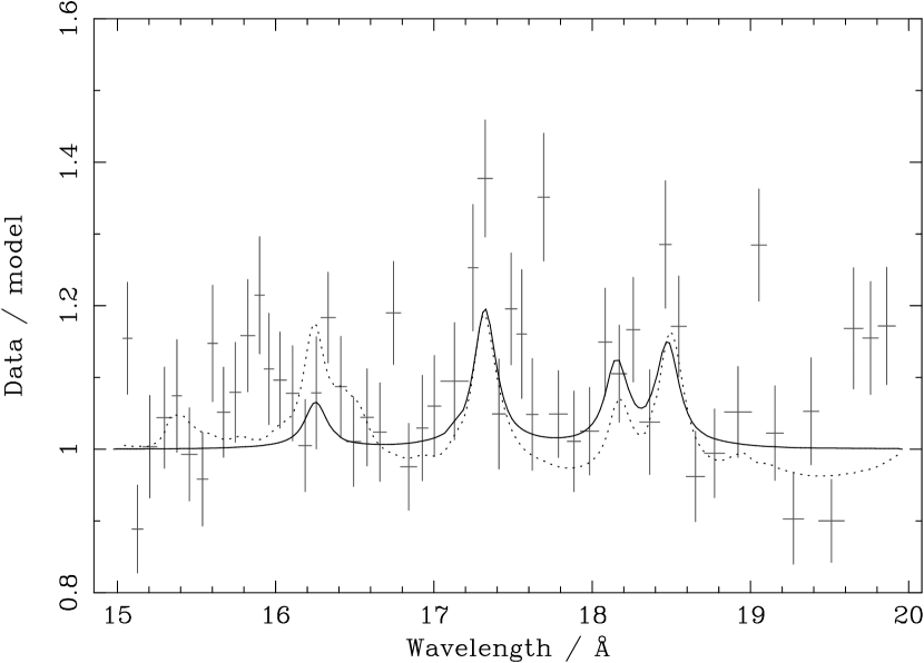
Figure 18: Ratio of data to a simple power-law model (i.e. no emission lines) in the 15–20 Å region. The data have been re-binned, and the two RGS instruments have been combined (this requires a degree of interpolation since the wavelengths bins in the two instruments do not coincide exactly), for display purposes only. The solid line shows the ratio appropriate for the Gaussian emission lines fitted in Table 4; the dotted line that for the cooling flow model C of Table 3. Note that the models were fitted to the un-binned data for the two separate instruments simultaneously (i.e. the models were not fitted to the data as displayed here).

In Fig. 18 we show the 15–20 Å region of the RGS spectrum, in terms of the ratio of the data to a model with no emission lines. Also shown are the appropriate curves for the model fitted for Table 4 (power-law plus Gaussians) and for model C of Table 3 (isobaric cooling flow). We note that the normalizations adopted by the Gaussians (where the line strengths may vary independently) are very similar to those of the cooling flow model. The exception is the 15.02 line, which is the Fe 17 line most susceptible to resonant scattering (e.g. Rugge & McKenzie, 1985, see also the APED database), for which a weaker fit is preferred. The quality of the line fits is clearly poor, but the values obtained for mass deposition rates agree with those from broad-band fits in both EPIC and the RGS.

6 Discussion

First, we must caution that the overall quality of our observation is low, and that the formal statistical significance of our results is not large. In particular, the results on the Fe 17 lines are really no more than suggestive. Nevertheless, the data do present a self-consistent picture between the various detectors, with an extremely interesting interpretation.

Fitting each of the three EPIC detectors individually for a large central region covering that radial range where the cluster emission is high, then the addition of a cooling flow component provides a highly significant improvement in fit over a single temperature model (although we cannot statistically distinguish a cooling flow component, with a range of temperatures, from a single temperature second component). The best-fitting mass deposition rate is around 90$\mathrm{\,\mathrm{\,M_{\odot}}}$$\mathrm{\,yr^{-1}}$, with a $1\sigma$ error of about 15$\mathrm{\,\mathrm{\,M_{\odot}}}$$\mathrm{\,yr^{-1}}$ (see Table 2 for details). The cooling time is less than 10$\mathrm{\,Gyr}$ within a radius of 130$\mathrm{\,kpc}$ (Fig. 9).

Very similar results are obtained from the broad-band simultaneous fit to the two RGS detectors (Table 3). The main evidence in the data for low-temperature gas comes from the spectral region around 15 Å, in particular the emission lines of Fe 17 at 15, 17 Å rest wavelength. We obtain weak (1–2$\sigma$; below formal detection levels) evidence for the three most important lines, and measure the power associated with each line (see Table 4). By comparing the line fluxes with those produced from a classical isobaric cooling flow model, we can estimate the corresponding mass-flow rate for each line. Once again, we obtain values that are consistent with the 90$\mathrm{\,\mathrm{\,M_{\odot}}}$$\mathrm{\,yr^{-1}}$ mark. Fixing the relative strengths of the three Fe lines to that predicted by the standard isobaric cooling flow model, and allowing the absolute normalization to vary, we obtain a fit suggesting the presence of Fe 17 at a significance of just over $2\sigma$.

We therefore establish, using three distinct methods, evidence for a cooling flow at a level $\sim 90\mathrm{\,\mathrm{\,M_{\odot}}}\mathrm{\,yr^{-1}}$. The preferred low-temperature cut-off for the flow, established from the RGS data, is essentially zero (0.081$\mathrm{\,keV}$, the minimum temperature available in the xspec mekal model). A plot of the $\dot{M}$–$T_{\mathrm{min}}$ confidence contours is shown in Fig. 17.

A re-analysis of the Chandra data for Abell 2597 (McNamara et al., 2001), as described in Section 3.1, also supports the existence of a cooling flow at these levels, with a very small low-temperature cut-off – see Fig. 4.

This mass deposition rate is consistent with the results of Oegerle et al. (2001), using FUSE UV observations. These authors detected the O 6 1032 Å resonance line (characteristic of gas at temperatures $\sim$ $3\times 10^{5}$$\mathrm{\,K}$) in Abell 2597. Converting the detected flux to an equivalent mass deposition rate gives a UV mass-deposition rate $\sim 40\mathrm{\,\mathrm{\,M_{\odot}}}\mathrm{\,yr^{-1}}$ within the FUSE effective radius of 40$\mathrm{\,kpc}$. This is consistent with the X-ray results (Fig. 7).

In contrast, O 6 was not detected in Abell 1795 (Oegerle et al., 2001), nor in Abell 2029 or Abell 3112 (Lecavelier des Etangs et al., 2004). Both from an X-ray and a UV standpoint, therefore, Abell 2597 appears to be an atypical object. The combination of the XMM-Newton X-ray and FUSE UV results for Abell 2597 suggests that it may harbour a classical cooling flow in which gas cools from $\sim$ 4$\mathrm{\,keV}$ by at least two orders of magnitude in temperature. Interestingly, a recent Chandra analysis of Abell 2029 (Clarke et al., 2004) shows that the X-ray data in this object are also consistent with a modest (by traditional standards) cooling flow extending down to very low temperatures, despite the lack of a UV detection.

Among the many (e.g. Fabian et al., 2001; Peterson et al., 2001) explanations suggested for the ‘cooling-flow problem’, heating from a central AGN, mediated by the rise of buoyant plasma bubbles through the ICM, is a popular candidate (e.g. Vecchia et al., 2004; Reynolds et al., 2005; Ruszkowski et al., 2004). The Chandra observation of Abell 2597 (McNamara et al., 2001) showed it to contain X-ray surface brightness depressions, interpreted (as a result of the extension of spurs of old, low-frequency radio emission) as ‘ghost cavities’, associated with a radio outburst $\sim 10^{8}$$\mathrm{\,yr}$ ago.

Abell 2597 therefore appears to harbour a central AGN that generates buoyant bubbles, and yet it also appears to contain gas cooling to very low temperatures. The process of bubble generation is necessarily an episodic one, and it therefore perhaps unreasonable to assume that a steady, time-independent state will be maintained. Clusters may go through cycles of behaviour, in which cooling builds up to some level, then an AGN outburst initiates a heating phase in which cooling is suppressed (else massive cooling flows would be common phenomena). Abell 2597 would then be an object near the ‘cooling catastrophe’ point of the cycle. The relative frequency of such objects would depend on the relative timescales of the cooling and heating phases. The fact that such objects seem to be quite rare indicates that the phase of strong cooling is short-lived.

Such a mechanism would require coupling between the state of the ICM and the activity of the central AGN, in order that a feedback loop could be maintained.

References

- Allen et al. (2001) Allen S. W., Fabian A. C., Johnstone R. M., Arnaud K. A., Nulsen P. E. J., 2001, MNRAS, 322, 589
- Allen et al. (2001) Allen S. W., Schmidt R. W., Fabian A. C., 2001, MNRAS, 328, L37
- Arnaud et al. (2001) Arnaud M., Neumann D. M., Aghanim N., Gastaud R., Majerowicz S., Hughes J. P., 2001, A&A, 365, L80
- Ball et al. (1993) Ball R., Burns J. O., Loken C., 1993, AJ, 105, 53
- Barnes & Nulsen (2003) Barnes D. G., Nulsen P. E. J., 2003, MNRAS, 343, 315
- Birkinshaw (1994) Birkinshaw M., 1994, in Crabtree D. R., Hanisch R. J., Barnes J., ed, Astronomical Data Analysis Software and Systems III, Vol. 61. ASP Conf. Ser., San Francisco, p. 249
- Bîrzan et al. (2004) Bîrzan L., Rafferty D. A., McNamara B. R., Wise M. W., Nulsen P. E. J., 2004, ApJ, 607, 800
- Clarke et al. (2004) Clarke T. E., Blanton E. L., Sarazin C. L., 2004, ApJ, 616, 178
- Crawford et al. (1989) Crawford C. S., Arnaud K. A., Fabian A. C., Johnstone R. M., 1989, MNRAS, 236, 277
- den Herder et al. (2001) den Herder J. W. et al., 2001, A&A, 365, L7
- Dickey & Lockman (1990) Dickey J. M., Lockman F. J., 1990, ARA&A, 28, 215
- Donahue et al. (2000) Donahue M., Mack J., Voit G. M., Sparks W., Elston R., Maloney P. R., 2000, ApJ, 545, 670
- Edge (2001) Edge A. C., 2001, MNRAS, 328, 762
- Edge et al. (2002) Edge A. C., Wilman R. J., Johnstone R. M., Crawford C. S., Fabian A. C., 2002, MNRAS, 337, 49
- Fabian (1994) Fabian A. C., 1994, ARA&A, 32, 277
- Fabian et al. (2001) Fabian A. C., Mushotzky R. F., Nulsen P. E. J., Peterson J. R., 2001, MNRAS, 321, L20
- Falcke et al. (1998) Falcke H., Rieke M. J., Rieke G. H., Simpson C., Wilson A. S., 1998, ApJ, 494, L155
- Freyberg et al. (2002a) Freyberg M. J., Briel U. G., Dennerl K., Haberl F., Hartner G., Kendziorra E., Kirsch M., 2002a, in Jansen F., ed, New Visions of the X-Ray Universe in the XMM-Newton and Chandra era. ESA SP-488, ESA Publications Division, Noordwijk
- Freyberg et al. (2002b) Freyberg M. J., Pfeffermann E., Briel U. G., 2002b, in Jansen F., ed, New Visions of the X-Ray Universe in the XMM-Newton and Chandra era. ESA SP-488, ESA Publications Division, Noordwijk
- Gastaldello et al. (2003) Gastaldello F., Ettori S., Molendi S., Bardelli S., Venturi T., Zucca E., 2003, A&A, 411, 21
- Ghizzardi (2001) Ghizzardi S., 2001, In flight calibration of the PSF for the MOS1 and MOS2 cameras, EPIC-MCT-TN-011
- Ghizzardi (2002) Ghizzardi S., 2002, In flight calibration of the PSF for the pn camera, EPIC-MCT-TN-012
- Gradshteyn & Ryzhik (2000) Gradshteyn I. S., Ryzhik I. M., 2000, Table of Integrals, Series, and Products (Sixth ed.). Academic Press
- Griffith et al. (1994) Griffith M. R., Wright A. E., Burke B. F., Ekers R. D., 1994, ApJS, 90, 179
- Heckman et al. (1989) Heckman T. M., Baum S. A., van Breughel W. J. M., McCarthy P., 1989, ApJ, 338, 48
- Jansen (2002) Jansen F., ed, 2002, New Visions of the X-Ray Universe in the XMM-Newton and Chandra era. ESA SP-488, ESA Publications Division, Noordwijk
- Johnstone et al. (2002) Johnstone R. M., Allen S. W., Fabian A. C., Sanders J. S., 2002, MNRAS, 336, 299
- Johnstone et al. (2005) Johnstone R. M., Fabian A. C., Morris R. G., Taylor G. B., 2005, MNRAS, 356, 237
- Kaastra et al. (2004) Kaastra J. S. et al., 2004, A&A, 413, 415
- Kirsch (2003) Kirsch M., 2003, EPIC status of calibration and data analysis, XMM-SOC-CAL-TN-0018
- Kirsch et al. (2004) Kirsch M. G. F. et al., 2004, XMM-Newton (cross)-calibration, XMM-SOC-CAL-TN-0055
- Koekemoer et al. (1999) Koekemoer A. M., O’Dea C. P., Sarazin C. L., McNamara B. R., Donahue M., Voit G. M., Baum S. A., Gallimore J. F., 1999, ApJ, 525, 621
- Kowalski et al. (1983) Kowalski M. P., Ulmer M. P., Cruddace R. G., 1983, ApJ, 268, 540
- Lecavelier des Etangs et al. (2004) Lecavelier des Etangs A., Gopal-Krishna , Durret F., 2004, A&A, 421, 503
- Lumb (2002) Lumb D., 2002, EPIC background files, XMM-SOC-CAL-TN-0016
- McNamara & O’Connell (1993) McNamara B. R., O’Connell R. W., 1993, AJ, 105, 417
- McNamara et al. (2001) McNamara B. R. et al., 2001, ApJ, 562, L149
- Mewe et al. (1995) Mewe R., Kaastra J. S., Liedahl D. A., 1995, Legacy, 6, 16
- Moos et al. (2000) Moos H. W. et al., 2000, ApJ, 538, L1
- Noonan (1981) Noonan T. W., 1981, ApJS, 45, 613
- O’Dea et al. (1994) O’Dea C. P., Baum S. A., Gallimore J. F., 1994, ApJ, 436, 669
- Oegerle et al. (2001) Oegerle W. R., Cowie L., Davidsen A., Hu E., Hutchings J., Murphy E., Sembach K., Woodgate B., 2001, ApJ, 560, 187
- Owen et al. (1995) Owen F. N., Ledlow M. J., Keel W. C., 1995, AJ, 109, 14
- Owen et al. (1992) Owen F. N., White R. A., Burns J. O., 1992, ApJS, 80, 501
- Peres et al. (1998) Peres C. B., Fabian A. C., Edge A. C., Allen S. W., Johnstone R. M., White D. A., 1998, MNRAS, 298, 416
- Peterson et al. (2003) Peterson J. R., Kahn S. M., Paerels F. B. S., Kaastra J. S., Tamura T., Bleeker J. A. M., Ferrigno C., Jernigan J. G., 2003, ApJ, 590, 207
- Peterson et al. (2001) Peterson J. R. et al., 2001, A&A, 365, L104
- Ponman et al. (2003) Ponman T. J., Sanderson A. J. R., Finoguenov A., 2003, MNRAS, 331
- Protassov et al. (2002) Protassov R., van Dyk D. A., Connors A., Kashyap V. L., Siemiginowska A., 2002, ApJ, 571, 545
- Reynolds et al. (2005) Reynolds C. S., McKernan B., Fabian A. C., Stone J. M., Vernaleo J. C., 2005, MNRAS, accepted (astro-ph/0402632)
- Rugge & McKenzie (1985) Rugge H. R., McKenzie D. L., 1985, ApJ, 297, 338
- Ruszkowski et al. (2004) Ruszkowski M., Brüggen M., Begelman M. C., 2004, ApJ, 615, 657
- Sakelliou et al. (2002) Sakelliou I. et al., 2002, A&A, 391, 903
- Sarazin et al. (1995) Sarazin C. L., Burns J. O., Roettiger K., McNamara B. R., 1995, ApJ, 447, 559
- Sarazin & McNamara (1997) Sarazin C. L., McNamara B. R., 1997, ApJ, 480, 203
- Saxton & Siddiqui (2002) Saxton R. D., Siddiqui H., 2002, The status of the SAS spectral response generation tasks for XMM-EPIC, XMM-SOC-PS-TN-43
- Schmidt (1965) Schmidt M., 1965, ApJ, 141, 1
- Soker (2003) Soker N., 2003, MNRAS, 342, 463
- Stark et al. (1992) Stark A. A., Gammie C. F., Wilson R. W., Bally J., Linke R. A., Heiles C., Hurwitz M., 1992, apjs, 79, 77
- Still & Mushotzky (2002) Still M., Mushotzky R., 2002, in Branduardi-Raymont G., ed, High Resolution X-Ray Spectroscopy with XMM-Newton and Chandra
- Struble & Rood (1999) Struble M. F., Rood H. J., 1999, ApJS, 125, 35
- Strüder et al. (2001) Strüder L. et al., 2001, A&A, 365, L18
- Tamura et al. (2003) Tamura T., den Herder J. W., González-Riestra R., 2003, RGS background files, XMM-SOC-CAL-TN-0034
- Taylor et al. (1999) Taylor G. B., O’Dea C. P., Peck A. B., Koekemoer A. M., 1999, ApJ, 512, L27
- Tozzi & Norman (2001) Tozzi P., Norman C., 2001, ApJ, 63
- Turner et al. (2001) Turner M. J. L. et al., 2001, A&A, 365, L27
- Vecchia et al. (2004) Vecchia C. D., Bower R. G., Theuns T., Balogh M. L., Mazzotta P., Frenk C. S., 2004, MNRAS, 355, 995
- Voit & Donahue (1997) Voit G. M., Donahue M., 1997, ApJ, 486, 242
- White (2000) White D. A., 2000, MNRAS, 312, 663
- Wright & Otrupcek (1990) Wright A., Otrupcek R., 1990, Parkes Catalogue (PKSCAT90)