Are PAHs precursors of small hydrocarbons in
Photo–Dissociation Regions? The Horsehead case

We present maps at high spatial and spectral resolution in emission lines of CCH, c-C₃H₂, C₄H, ¹²CO and C¹⁸O of the edge of the Horsehead nebula obtained with the Plateau de Bure Interferometer (PdBI). The edge of the Horsehead nebula is a one-dimensional Photo–Dissociation Region (PDR) viewed almost edge-on. All hydrocarbons are detected at high signal–to–noise ratio in the PDR where intense emission is seen both in the H₂ ro-vibrational lines and in the PAH mid–infrared bands. C¹⁸O peaks farther away from the cloud edge. Our observations demonstrate that CCH, c-C₃H₂ and C₄H are present in UV–irradiated molecular gas, with abundances nearly as high as in dense, well shielded molecular cores.
PDR models i) need a large density gradient at the PDR edge to correctly reproduce the offset between the hydrocarbons and H₂ peaks and ii) fail to reproduce the hydrocarbon abundances. We propose that a new formation path of carbon chains, in addition to gas phase chemistry, should be considered in PDRs: because of intense UV–irradiation, large aromatic molecules and small carbon grains may fragment and feed the interstellar medium with small carbon clusters and molecules in significant amount.

1 Introduction

Due to the ISO mission, the knowledge of interstellar dust has significantly progressed in the past years. With its sensitive instruments in the mid–infrared, ISO revealed the spatial distribution and line profile of the Aromatic Infrared Bands (AIBs at 3.3, 6.2, 7.7, 8.6 and 11.3 $\mu m$ features), which have shed light on the emission mechanism and their possible carriers (Boulanger et al. 2000; Rapacioli et al. 2004). However, no definite identification of individual species has been possible yet because the bands are not specific for individual molecules. The most likely carriers are large polycyclic aromatic hydrocarbons (PAHs) with about 50 carbon atoms (Allain et al. 1996b; Le Page et al. 2003). The ubiquity of the aromatic band emission in the interstellar medium has triggered a wealth of theoretical and laboratory work in the past two decades, which have led to a revision of astrophysical models. PAHs are now suspected to play a major role in both the interstellar medium physics and chemistry. With their small size, they are the most efficient particles for the photo–electric effect (Bakes & Tielens 1994; Weingartner & Draine 2001; Habart et al. 2001). Their presence also affects the ionization balance (Flower & Pineau des Forêts 2003; Wolfire et al. 2003), and possibly the formation of H₂ (Habart et al. 2004). The role of PAHs in the neutralization of atomic ions in the diffuse interstellar medium has been recently reconsidered by Liszt (2003), following previous work by Lepp et al. (1988). As emphasized soon after their discovery (Omont 1986; Lepp & Dalgarno 1988), PAHs also play a role in the gas chemistry: a few laboratory experiments, and theoretical calculations, suggest that PAHs may fragment into small carbon clusters and molecules under photon impact (C₂, C₃, C₂H₂, etc.) (Joblin 2003; Le Page et al. 2003; Allain et al. 1996b, a; Leger et al. 1989; Scott et al. 1997). In addition, investigation of the lifetimes of interstellar PAHs implies that photo–dissociation may be the main limiting process for their life in the interstellar medium (Verstraete et al. 2001).

It is therefore appropriate to wonder whether PAHs could fragment continuously and feed the interstellar medium with small hydrocarbons and carbon clusters. This hypothesis is attractive for the following reasons:

• Cyclopropenylidene (c-C₃H₂) is widely distributed in the interstellar medium (Matthews & Irvine 1985; Matthews et al. 1986; Cox et al. 1988; Lucas & Liszt 2000).

• Recent works have shown that the diffuse interstellar medium is more chemically active than previously thought with molecules as large as C₃ (Goicoechea et al. 2004; Oka et al. 2003; Ádámkovics et al. 2003; Roueff et al. 2002; Maier et al. 2001) and c-C₃H₂ (Lucas & Liszt 2000) widely distributed. The abundance of C₃ and c-C₃H₂ are tightly connected with those of smaller molecules, C₂ and CCH respectively, with abundance ratios of [C₂]/[C₃] $\sim 10-40$ (Oka et al. 2003) and [CCH]/[c-C₃H₂] $\sim 27.7\pm 8$ (Lucas & Liszt 2000).

• Thorburn et al. (2003) have found a correlation between the abundance of C₂ and the strength of some (weak) Diffuse Interstellar Bands (DIBs).

As PAHs are present in the diffuse interstellar medium, could they contribute in forming both the small carbon clusters (C₂, C₃) and larger hydrocarbon molecules which could be the DIBs carriers?

Unfortunately, studies of the PAHs emission bands in the diffuse interstellar clouds where the carbon clusters have been detected is extremely difficult because of the low column densities, and also because the bright background star used for visible spectroscopy prohibits the use of sensitive IR cameras which would be saturated. Photo–Dissociation regions (PDRs) are the first interstellar sources in which the AIBs have been found and the PAHs hypothesis proposed (Sellgren 1984; Leger & Puget 1984). It is therefore interesting to investigate the carbon chemistry in these sources. Fossé et al. (2000) and Teyssier et al. (2004) have discussed medium spatial resolution ($30^{\prime\prime}$) observations of various hydrocarbons in nearby PDRs. They show that CCH, c-C₃H₂ and C₄H are ubiquitous in these regions, with abundances almost as high as in dark, well shielded, clouds, despite the strong UV–radiation. Fuente et al. (2003) also report high abundances of c-C₃H₂ in NGC 7023 and the Orion Bar. Heavier molecules may be present in PDRs as Teyssier et al. (2004) report a tentative detection of C₆H in the Horsehead nebula. PDRs and diffuse clouds therefore seem to share the same carbon chemistry, but because of their larger H₂ column density and gas density, PDRs offer more opportunities for detecting rare species.

Teyssier et al. (2004) and Fuente et al. (2003) reckon the presence of carbon chains is in favor of a causal link between small hydrocarbons and PAHs, but they lack the spatial resolution to conclude. In the present work, we present high spatial resolution observations of one source studied by Teyssier et al. (2004), the Horsehead nebula, obtained with the Plateau de Bure interferometer. We describe the observations in Sec. 2. We show the interferometer maps in Sec. 3. Finally, Sec. 4 presents a comparison with chemical models.

2 Observations and data reduction

2.1 The Horsehead nebula

The Horsehead nebula, also called Barnard 33, appears as a dark patch of $\sim 5^{\prime}$ extent against the bright HII region IC434. Emission from the gas and dust associated with this globule has been detected from mid–IR to millimeter wavelengths (Abergel et al. 2002, 2003; Teyssier et al. 2004; Pound et al. 2003). From the analysis of the ISOCAM images, Abergel et al. (2003) conclude that the Horsehead nebula is a PDR viewed edge-on and illuminated by the O9.5V star $\sigma$Ori at a projected distance of 0.5^∘ (3.5$\,\mathrm{pc}$ for a distance of 400$\,\mathrm{pc}$, Anthony-Twarog (1982)). The far–UV intensity of the incident radiation field is $G_{0}=60$ relative to the average interstellar radiation field in Draine units (Draine 1978). The gas density, derived from the excitation of molecular lines, and from the penetration depth of the UV–radiation, is a few $10^{4}\,\mathrm{cm^{-3}}$ (Abergel et al. 2003). From a combined analysis of maps of both CO and atomic carbon, Lis & Guesten (2005) obtain similar figures for the gas density. Habart et al. (2004, 2005) have modeled the emission of H₂ (from narrow band images of H₂ ro-vibrational line), PAHs and CO, and conclude that i) the gas density follows a steep gradient at the cloud edge, rising to $n_{\mathrm{H}}=10^{5}\,\mathrm{cm^{-3}}$ in less than $10^{\prime\prime}$ (i.e. 0.02$\,\mathrm{pc}$) and ii) this density gradient model is essentially a constant pressure model (with $P=4\times 10^{6}\,\mathrm{K\,km\,s^{-1}}$).

The edge of the Horsehead nebula is particularly well delineated by the mid–IR emission due to PAHs, with a bright 7.7$\,\mathrm{\mu m}$–peak (hereafter named “IR peak”) reaching 25 MJy/sr at $\alpha_{2000}=05^{h}40^{m}53.70^{s},\delta_{2000}=-02^{\circ}28^{\prime}04^{\prime\prime}$. Fig. 1 shows the region observed with the IRAM PdBI centered near the “IR peak”. Two mosaics (one for hydrocarbon lines and the other for the CO lines) have been observed. Their set-ups are detailed in Table 1.

Table 1: Observation parameters.

	Phase center		Number of fields
Mosaic 1	$\alpha_{2000}=05^{h}40^{m}54.27^{s}$	$\delta_{2000}=-02^{\circ}28^{\prime}00^{\prime\prime}$	7
Mosaic 2	$\alpha_{2000}=05^{h}40^{m}53.00^{s}$	$\delta_{2000}=-02^{\circ}28^{\prime}00^{\prime\prime}$	4

Molecule & Line	Frequency	Beam	PA	Noisea	Obs. date
	GHz	arcsec	∘	$\,\mathrm{K\,km\,s^{-1}}$
Mosaic 1
c-C3H2 $2_{1,2}-1_{0,1}$	85.339	$6.13\times 4.75$	36	3.1$\times 10^{-2}$	Mar. 2002 & Apr. 2002
C4H-1 N=9-8,J=19/2-17/2	85.634	$6.11\times 4.74$	36	2.6$\times 10^{-2}$	Mar. 2002 & Apr. 2002
C4H-2 N=9-8,J=17/2-15/2	85.672	$6.11\times 4.74$	36	3.4$\times 10^{-2}$	Mar. 2002 & Apr. 2002
CCH-1 N=1-0, J=3/2-1/2 F=2-1	87.316	$7.24\times 4.99$	54	3.4$\times 10^{-2}$	Dec. 2002 & Mar. 2003
CCH-2 N=1-0, J=3/2-1/2 F=1-0	87.328	$7.24\times 4.99$	54	2.5$\times 10^{-2}$	Dec. 2002 & Mar. 2003
CCH-3 N=1-0, J=1/2-1/2 F=1-1	87.402	$7.24\times 4.99$	54	3.4$\times 10^{-2}$	Dec. 2002 & Mar. 2003
CCH-4 N=1-0, J=1/2-1/2 F=0-1	87.407	$7.24\times 4.99$	54	2.3$\times 10^{-2}$	Dec. 2002 & Mar. 2003
C18O J=2–1	219.560	$6.54\times 4.31$	65	9.8$\times 10^{-2}$	Mar. 2003
Mosaic 2
12CO J=1–0	115.271	$5.95\times 5.00$	65	1.2$\times 10^{-1}$	Nov. 1999
12CO J=2–1	230.538	$2.97\times 2.47$	66	1.7$\times 10^{-1}$	Nov. 1999

^a The noise values quoted here are the noises at the mosaic center (Please remember that mosaic noise is inhomogeneous due to primary beam correction: It steeply increases at the mosaic edges). Those noise values have been computed on 1$\,\mathrm{km\,s^{-1}}$ velocity bin.

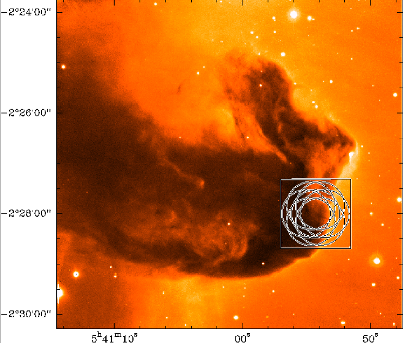
Figure 1: The field of view covered when mapping small hydrocarbons at 3.4$\,\mathrm{mm}$ with the Plateau de Bure Interferometer (PdBI) is shown as a square over this ESO–VLT composite image (B, V and R bands) of the Horsehead nebula. Each circle features the 3.4$\,\mathrm{mm}$ primary beam of the PdBI at one of the 7 observed positions. Those positions are largely oversampled at the hydrocarbon wavelength (3.4$\,\mathrm{mm}$) to ensure simultaneous Nyquist-sampling at 1.4$\,\mathrm{mm}$ used to observe C¹⁸O. A linear combination of the 7 pointed observation is done to obtain the final dirty image.

2.2 Observations

2.2.1 c-C₃H₂ and C₄H

First PdBI observations dedicated to this project were carried out with 6 antennas in CD configuration (baseline lengths from 24 to 229 m) during March–April 2002. The 580$\,\mathrm{MHz}$ instantaneous IF–bandwidth allowed us to observe simultaneously c-C₃H₂ and C₄H at 3$\,\mathrm{mm}$ using 3 different 20$\,\mathrm{MHz}$–wide correlator windows. One other window was centered on the C¹⁸O (J=2–1) frequency. The full IF bandwidth was also covered by continuum windows both at 3.4 and 1.4$\,\mathrm{mm}$. c-C₃H₂ and C₄H were detected but the weather quality precluded use of 1.4$\,\mathrm{mm}$ data.

We observed a seven–field mosaic on a compact, hexagonal pattern, with full Nyquist sampling at 1.4 mm and large oversampling at 3.4 mm. This mosaic, centered on the IR peak, was observed during about 6h on–source observing time per configuration. The rms phase noises were between 15 and 40^∘ at 3.4$\,\mathrm{mm}$, which introduced position errors $<0.5^{\prime\prime}$. Typical 3.4$\,\mathrm{mm}$ resolution was $6^{\prime\prime}$.

2.2.2 CCH and C¹⁸O

Table 2: Calibrator fluxes in Jy.

	B0420$-$014		B0607$-$157		B0528$+$134
	3$\,\mathrm{mm}$	1$\,\mathrm{mm}$	3$\,\mathrm{mm}$	1$\,\mathrm{mm}$	3$\,\mathrm{mm}$	1$\,\mathrm{mm}$
27.11.1999					3.5	1.4
30.03.2002	4.8		2.3
16.04.2002	4.8		2.5
22.04.2002	4.8		2.4
23.12.2002	12.5		2.6
18.03.2003	12.0	7.8	2.1	0.87
26.03.2003	12.8		2.1

As a follow-up, we carried out observations of CCH at PdBI with 6 antennas in CD configuration during December 2002 and March 2003. We used a similar correlator setup: three 20$\,\mathrm{MHz}$–wide windows were centered so as to get the four 3.4$\,\mathrm{mm}$ hyperfine components of CCH; one 20$\,\mathrm{MHz}$–wide window was centered on the C¹⁸O (J=2–1) frequency; the remaining windows were used to observe continuum at 3.4 and 1.4$\,\mathrm{mm}$.

Exactly the same mosaic (center and field–pattern) and approximately the same on–source observing time per configuration ($\sim$ 6h) as before were used. The rms phase noises were between 10 and 40^∘ except during 4 hours in D configuration where they were between 8 and 20^∘ at 3.4$\,\mathrm{mm}$. The data of those 4 hours have been used to build the C¹⁸O map as the 1$\,\mathrm{mm}$ phase noises were then low enough (between 20 to 45^∘). We thus ended up with a $6^{\prime\prime}$ typical resolution both at 3.4$\,\mathrm{mm}$ and 1.4$\,\mathrm{mm}$. Both CCH and C¹⁸O were easily mapped while no continuum was detected at a level of 2 mJy/beam in a $6^{\prime\prime}$–beam.

2.2.3 ¹²CO

As part of another project (A. Abergel, private communication), the ¹²CO (J=1–0) and ¹²CO (J=2–1) lines were simultaneously observed during 6h on–source at PdBI in November 1999 (only 5 antennas were then available) in configuration C (baseline lengths from 24 to 82 m).

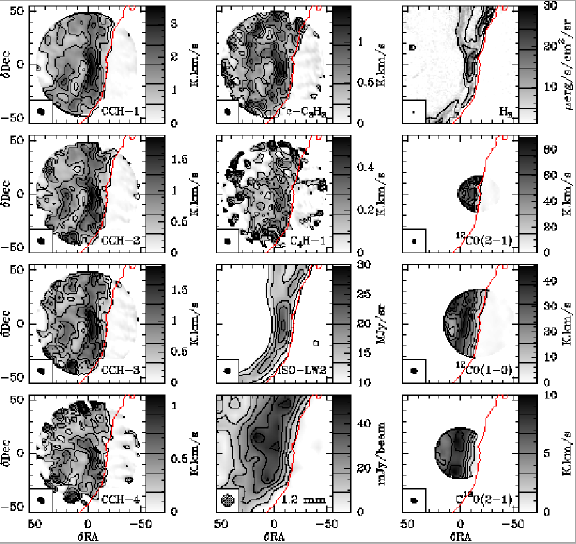
Figure 2: Integrated emission maps obtained with the Plateau de Bure Interferometer. Maps of i) the H₂ v=1-0 S(1) emission (Habart et al. 2004, 2005), ii) the mid–IR emission (Abergel et al. 2003, labeled ISO-LW2) and iii) the 1.2$\,\mathrm{mm}$ dust continuum (Teyssier et al. 2004, labeled 1.2mm) are also shown for comparison. The center of all maps has been set to the mosaic 1 phase center: RA(2000) = 05h40m54.27s, Dec(2000) = -02^∘28’00^′′. The map size is $110^{\prime\prime}\times 110^{\prime\prime}$, with ticks drawn every $10^{\prime\prime}$. Either the synthesized beam or the single dish beam is plotted in the bottom, left corner. The emission of all the lines observed at PdBI is integrated between 10.1 and 11.1 $\,\mathrm{km\,s^{-1}}$. Values of contour level are shown on each image wedge (contours of the H₂ image have been computed on an image smoothed to $5^{\prime\prime}$ resolution). The sharp edge of the H₂ emission (upper right panel) defines a boundary, which is used as a numerical support (in the language of signal processing) for deconvolution of the other images. This deconvolution support is overplotted in red on every panel.

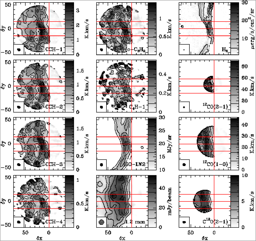
Figure 3: Same as Fig. 2 except that maps have been rotated of 14^∘ counter–clockwise around the image center to bring the exciting star direction in the horizontal direction as this eases the comparison of the PDR tracer stratifications. Maps have also been horizontally shifted by $20^{\prime\prime}$ to set the horizontal zero at the PDR edge delineated as the vertical red line. Horizontal red lines delimit the two lanes that have been vertically averaged to produce the two series of cuts shown in Fig. 5.

The observation consisted in a 4–fields mosaic, fully sampled at 1.3$\,\mathrm{mm}$. The mosaic center is slightly shifted compared to the two other observations. Weather was excellent with phase noises from 3 to 5^∘ and 6 to 10^∘ at 2.6$\,\mathrm{mm}$ and 1.3$\,\mathrm{mm}$, respectively. Typical resolutions were $5^{\prime\prime}$ at 2.6$\,\mathrm{mm}$ and $2.5^{\prime\prime}$ at 1.3$\,\mathrm{mm}$.

2.2.4 Other data: H₂, ISO-LW2 and 1.2$\,\mathrm{mm}$ dust continuum

The H₂ v=1-0 S(1) map shown here is a small part of Horsehead observations obtained at the NTT using SOFI. The resolution is $\sim 1^{\prime\prime}$. Extensive explanations of data reduction and analysis are discussed elsewhere (Habart et al. 2004, 2005). The ISO-LW2 map (published by Abergel et al. (2003)) shows aromatic features at $7.7\mu m$ with a resolution of $\sim 6^{\prime\prime}$. The 1.2$\,\mathrm{mm}$ dust continuum has been obtained at the IRAM-30m telescope with a resolution of $\sim 11^{\prime\prime}$ and has already been presented by Teyssier et al. (2004).

2.3 PdBI data processing

All data reduction was done with the GILDAS softwares supported at IRAM. Standard calibration methods using close calibrators were applied to all the PdBI data. The calibrator fluxes used for the absolute flux calibration are summarized in Table 2.

Following Gueth et al. (1996), single–dish, fully sampled maps obtained at the IRAM-30m telescope (Teyssier et al. 2004; Abergel et al. 2003)) were used to produce the short–spacing visibilities filtered out by every mm-interferometer (e.g. spatial frequencies between 0 and 15$\,\mathrm{m}$ for PdBI). Those pseudo-visibilities were merged with the observed, interferometric ones. Each mosaic field were then imaged and a dirty mosaic was built combining those fields in the following optimal way in terms of signal–to–noise ratio (Gueth 2001):

$$J(\alpha,\delta)=\sum\nolimits_{i}\frac{B_{i}(\alpha,\delta)}{\sigma_{i}^{2}}\,F_{i}(\alpha,\delta)\left/\displaystyle\sum\nolimits_{i}\frac{B_{i}(\alpha,\delta)^{2}}{\sigma_{i}^{2}}.\right.$$

In this equation, $J(\alpha,\delta)$ is the brightness distribution in the dirty mosaic image, the $B_{i}$ are the response functions of the primary antenna beams, the $F_{i}$ are the brightness distributions of the individual dirty maps, and the $\sigma_{i}$ are the corresponding noise values. As may be seen on this equation, the dirty intensity distribution is corrected for primary beam attenuation. This implies that noise is inhomogeneous. In particular, noise strongly increases near the edges of the field of view. To limit this effect, both the primary beams used in the above formula and the resulting dirty mosaics are truncated. Standard level of truncation is set to 20% of the maximum in GILDAS. In our case, the intensity distribution does not drop to zero at all field edges. Hence, we used a much lower level of truncation of the beam (i.e. 5%) to ensure a better deconvolution of the side lobes of the sources sitting just at the field edges. We then use the standard adaptation to mosaics of the Högbom CLEAN algorithm to deconvolve (Gueth 2001). The sharp edge of the H₂ emission defines a boundary that may be used as an a priori knowledge in the deconvolution of the PdBI images: We use this boundary as a numerical support (in the language of signal processing) to forbid the search of CLEAN components outside the PDR front (i.e. in the direction of the exciting star). We finally truncated the noisy clean mosaic edges using the standard truncation level. It may be noted that the C₄H maps are particularly difficult to deconvolve due to their low signal–to–noise ratio, $S/N<10$ to 15.

3 Results

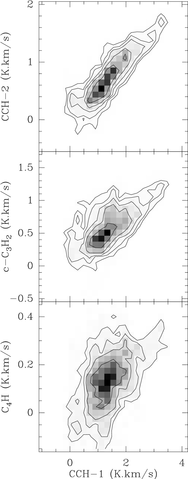
Figure 4: Joint histogram of the integrated emission of i) the second brightest CCH line (top), ii) c-C₃H₂ (middle) and iii) one C₄H line (bottom) vs. the main CCH line. The value at a given position of this joint histogram is the percentage of pixels of the input images whose intensities lies in the respective vertical and horizontal bins. Only image pixels lying inside the deconvolution support (shown in Fig. 2) have been used in the histogram computation. Contour levels are set to 0.125, 0.25, 0.5, 1, 2, 4 and 8% of points per pixel.

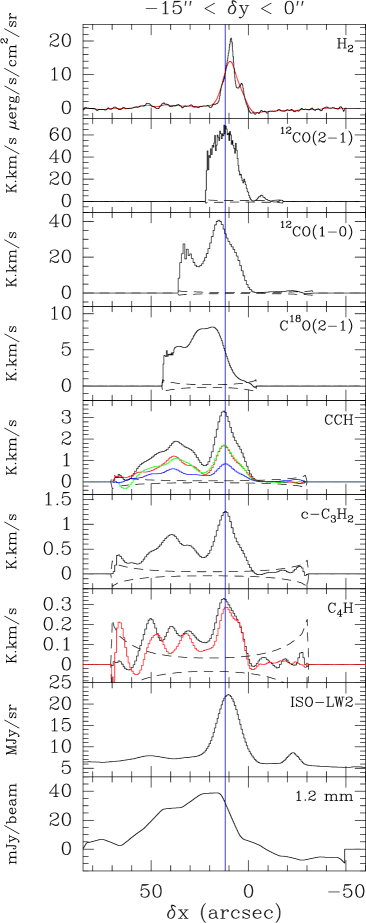
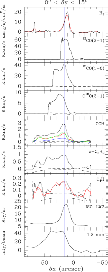
Figure 5: Emission profiles along the exciting star direction (PA = -104^∘ in equatorial coordinate system). To improve signal–to–noise ratio, those emission profiles have been integrated along the perpendicular direction between $-15^{\prime\prime}<\delta y<0^{\prime\prime}$ (left column) and $0^{\prime\prime}<\delta y<+15^{\prime\prime}$ (right column). The comparison of those two series of mean cuts gives an idea of the influence of the local conditions (either excitation effects or chemical differentiation). We show from top to bottom, H₂ v=1-0 S(1) (full resolution in black, smoothed at a $5^{\prime\prime}$–resolution in red), ¹²CO J=2–1, ¹²CO J=1–0, C¹⁸O J=2–1, CCH lines (1 black, 2 green, 3 red and 4 blue, respectively following the ratios 1:0.5:0.5:0.25), c-C₃H₂, C₄H lines (1 black, 2 red), ISO-LW2 and the 1.2$\,\mathrm{mm}$ dust continuum. For the PdBI data, the 3–$\sigma$ noise level is indicated by the dashed lines. It rises at the cut edges due to the primary beam correction. Note that the fields of view of the ¹²CO and C¹⁸O data are smaller than the field of view of the hydrocarbon data because of the smaller mosaic size and/or the higher frequency. Finally, the blue vertical lines give guideline to localize the hydrocarbon peaks. They have been drawn at $\delta x=+12^{\prime\prime}$ (left column) and $\delta x=+15^{\prime\prime}$ (right column). Note that the bumps at $\delta x=-20^{\prime\prime}$ in the ISO-LW2 cut (left column) and at $\delta x=70^{\prime\prime}$ in the H₂ cut (right column) are due to field stars.

3.1 Maps

The PdBI maps are shown in Fig. 2 and 3 together with the 7$\,\mathrm{\mu m}$ ISOCAM image (Abergel et al. 2003), the 1.2$\,\mathrm{mm}$ dust emission map (Teyssier et al. 2004) and the map of the H₂ 2.1$\,\mathrm{\mu m}$ line emission (Habart et al. 2004, 2005) for comparison. For all lines, we obtained excellent spatial resolutions, similar to or even better than the ISOCAM pixel size of $6^{\prime\prime}$ (see Table 1). Fig. 2 shows the maps in the natural Equatorial coordinate system while Fig. 3 shows the maps in a coordinate system where the x-axis is in the direction of the exciting star and the y-axis defines an empirical PDR edge that corresponds to the sharp boundary of the H₂ emission (i.e. the maps have been rotated by 14^∘ counter-clockwise and horizontally shifted by $20^{\prime\prime}$). The latter presentation enables a much better comparison of the PDR stratification.

The main structure in all hydrocarbon maps is an approximatively N-S filament, following nicely the cloud edge and corresponding closely to the mid–IR filament on the ISO-LW2 image. A weaker and more extended emission is also detected, which has no counterpart in the ISO-LW2 image and can be attributed to the bulk of the cloud. It is interesting to note that the hydrocarbon emission presents a minimum behind the main filament, and a weaker secondary maximum within the extended emission. The hydrocarbon emission is stronger on the edges of the dust 1.2$\,\mathrm{mm}$ emission and avoids the region of maximum dust emission where the gas is likely denser. This confirms a tendency revealed by chemical surveys of dense cores (study of TMC-1 by Pratap et al. (1997) and L134N by Dickens et al. (2000); Fossé (2003)): i.e. carbon chains (CCH, C₄H,…) generally avoid the densest and more depleted cores.

Even at the high spatial resolution provided by the plateau de Bure Interferometer, the maps of all hydrocarbons remain very similar. Detailed inspection of the maps shows small differences between CCH and c-C₃H₂, but these do not affect the overall similarity. Indeed, the joint histogram describing the correlation of line maps for i) the two most intense CCH lines, ii) c-C₃H₂ and CCH, and iii) C₄H and CCH are displayed in Fig. 4. As expected the two CCH lines are extremely well correlated as illustrated by the elongated shape (approaching a straight line) of the joint histogram. The correlations between c-C₃H₂ and CCH, and between C₄H and CCH are excellent too, though the signal–to–noise ratio is not as good for C₄H. For this plot, we have used all points lying inside the support used for the deconvolution.

The high resolution c-C₃H₂ map appears to show more structure than the CCH maps, particularly in the well shielded cloud interior (on the left hand side of the main filament). This effect seems real since it does not appear for the satellite CCH line maps, which have similar intensities and signal–to–noise ratio as the c-C₃H₂ map. The C₄H maps are too noisy for a detailed analysis but are nevertheless very well correlated with the CCH map. The correlations found at low spatial resolution (Teyssier et al. 2004) are not an artifact but persist at high spatial resolution.

The correspondence of hydrocarbons with CO and C¹⁸O is not as good. The C¹⁸O (J=2–1) map presents two maxima, located on either side of the CCH peak along a N-S direction: The CCH peak is associated with a local minimum of C¹⁸O emission. Also, the C¹⁸O emission peak is displaced farther inside the cloud (East) compared to CCH and the other hydrocarbons.

To illustrate further the differences in the spatial distribution of CO, C¹⁸O and the hydrocarbons, we show two series of cuts across the PDR in Fig. 5. The UV–radiation comes from $\sigma$ Ori far to the right side of the Fig. 3. The cuts have been taken along the $\sigma$ Ori direction (i.e. PA$=-104^{\circ}{}$). The main peak for all hydrocarbons is located near an offset of $\delta x\simeq 12-15\arcsec$ at less than $5^{\prime\prime}$ of the H₂ peak. The ISO-LW2 peak is located half–way between hydrocarbons and H₂ peaks. Intense ¹²CO emission, in both the J=1–0 and J=2–1 lines is also detected in the same region, while the C¹⁸O (J=2–1) emission rises farther (at least $5^{\prime\prime}$) inside the cloud.

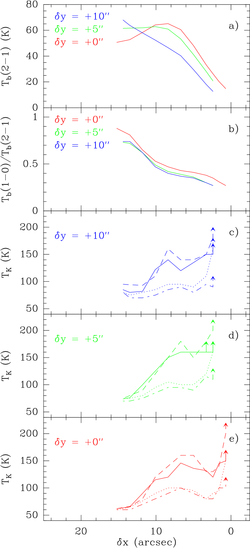
Figure 6: Spatial variation along the direction of the exciting star of a) the ¹²CO J=2–1 brightness temperature (convolved at the same angular resolution as the J=1–0 transition), b) 1-0/2-1 ratio and c,d,e) the kinetic temperature. $(\delta x,\delta y)$ offsets refer to the coordinate system defined in Fig. 3. The cuts at $\delta y=+10^{\prime\prime}$ are drawn in blue, those at $\delta y=+5^{\prime\prime}$ in green and those $\delta y=+0^{\prime\prime}$ in red. The data cuts have been taken from the 10.6$\,\mathrm{km\,s^{-1}}$ velocity channel corresponding to the ¹²CO line peak. The kinetic temperature is derived from an LVG model assuming i) unity beam filling factor and ii) uniform total hydrogen density of $n_{\mathrm{H}}=1.6\times 10^{4}\,\mathrm{cm^{-3}}$ (dashed lines), $2\times 10^{4}\,\mathrm{cm^{-3}}$ (full lines), $4\times 10^{4}\,\mathrm{cm^{-3}}$ (dotted lines) and $10^{5}\,\mathrm{cm^{-3}}$ (dotted–dashed lines). Arrows indicate lower limits.

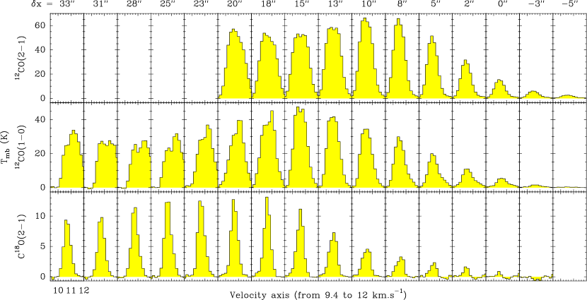
Figure 7: CO spectra (convolved at the same angular resolution) along the direction of the exciting star at $\delta y=-2.5^{\prime\prime}$. In those cuts, the label $\delta x=13^{\prime\prime}$ indicates the IR peak position (cf. table 3). Note that ¹²CO J=2–1 peak intensity decreases at positions $\delta x=13^{\prime\prime}$ and $15^{\prime\prime}$ while ¹²CO J=1–0 increases even reaching its maximum at $\delta x=15^{\prime\prime}$. In addition, both ¹²CO lines show a small but clear dip (i.e. the center channel intensity is lower than its first neighbours) at $\delta x=15^{\prime\prime}$. Finally, while C¹⁸O spectra are very close to Gaussians, ¹²CO spectra show asymmetric profiles. Spectra cuts at other close $\delta y$ values show the same trends.

As shown in Fig. 6, the ¹²CO (J=2–1) emission (convolved at the same angular resolution as the ¹²CO J=1–0 transition) is very bright ($\geq 50\,\mathrm{K}{}$ at $10.6\,\mathrm{km\,s^{-1}}$, the line peak velocity) and more intense than ¹²CO (J=1–0) in the most external layers of the PDRs, facing directly $\sigma$Ori. The line intensity ratio $T_{b}(1-0)/T_{b}(2-1)$ rises from $\sim 0.3$ to $\sim 0.8$ from West to East. Combined with the high brightness temperature detected for both lines, the higher brightness temperature of the ¹²CO(2-1) line is a clear sign of the presence of warm and dense gas. We have estimated the kinetic temperature using an LVG model. We assumed that the emission is resolved and fills the beam. We explored the kinetic temperature dependence upon the density by solving for 5 different proton densities going from $1.6\times 10^{4}\,\mathrm{cm^{-3}}$ to $10^{5}\,\mathrm{cm^{-3}}$. Under these hypotheses, the ¹²CO line intensity ratio and brightness temperature constrain the kinetic temperature to increase from $60\,\mathrm{K}$ in the inner PDR ($15^{\prime\prime}=0.03\,\mathrm{pc}$ from the PDR edge) to more than $100\,\mathrm{K}$ in the outer layers for proton densities larger than $4\times 10^{4}\,\mathrm{cm^{-3}}$. For lower proton densities, the kinetic temperature still starts from $60\,\mathrm{K}$ in the inner PDR but increases much more stiffly. The kinetic temperature derived from single dish observations (Abergel et al. 2003) is lower, in the $30-40\,\mathrm{K}$ range and corresponds to the bulk of the cloud, rather than to the warm UV–illuminated edge.

3.2 Abundances

We have computed the CO and hydrocarbons column densities at three representative positions in the maps: the “IR peak” where the PAH and hydrocarbon emission is the largest, the “IR edge” $10^{\prime\prime}$ West which represents the region with the most intense UV–radiation and a “Cloud” position behind the IR filament. Table 3 lists the derived column densities and abundances relative to the total number of protons for these 3 positions. We have used a LVG model with different uniform total hydrogen density (from $10^{4}\,\mathrm{cm^{-3}}$ to $10^{5}\,\mathrm{cm^{-3}}$) and a kinetic temperature of 40$\,\mathrm{K}$ for the “cloud” position, and between 60 and 100$\,\mathrm{K}$ for the IR positions. The variance of the column densities therefore reflects both the systematic effect due to the imperfect knowledge of the physical conditions, and the random noise of the data. In most cases, the former contribution is the largest. The H₂ column densities are derived from the dust 1.2$\,\mathrm{mm}$ emission assuming the same dust properties for all positions but a dust temperature range of 20 to 40$\,\mathrm{K}$ for the “Cloud” position and 40 to 80$\,\mathrm{K}$ for the IR positions.

Table 3: Molecular column densities and abundances at 3 different positions of the PDR named “Cloud”, “IR peak” and “IR edge”. Equatorial offsets refer to the Mosaic 2 map center given in Table 1. $(\delta x,\delta y)$ offsets refer to the coordinate system defined in Fig. 3. H₂ column densities have been derived from the 1.2$\,\mathrm{mm}$ dust continuum emission using a dust temperature range of 20 to 40$\,\mathrm{K}$ for the “Cloud” position and 40 to 80$\,\mathrm{K}$ for the IR positions. Others column densities used LVG models with a representative set of densities and kinetic temperature. 1–$\sigma$ uncertainties thus reflect the systematics due to the approximate knowledge of density and kinetic temperature. Abundances are computed with respect to the number of protons, i.e. $[X]=0.5\,N(X)/N(\mbox{H${}_{2}$})$.

	$\delta$RA	$\delta$Dec	$\delta x$	$\delta y$
Cloud	$+6^{\prime\prime}$	$-4^{\prime\prime}$	$+24.9^{\prime\prime}$	$-5.3^{\prime\prime}$
IR peak	$-6^{\prime\prime}$	$-4^{\prime\prime}$	$+12.2^{\prime\prime}$	$-2.4^{\prime\prime}$
IR edge	$-12^{\prime\prime}$	$-4^{\prime\prime}$	$+7.4^{\prime\prime}$	$-1.0^{\prime\prime}$

Quantity	Unit	Cloud		IR peak		IR edge
$S_{1.2\,\mathrm{mm}}$	mJy/Beam	38$\pm$	2	35$\pm$	2	12$\pm$	2
$N(\mbox{H${}_{2}$})$	1021$\,\mathrm{cm^{-2}}$	27$\pm$	9.5	10.5$\pm$	4	3.6$\pm$	1.7
$N(\mbox{C${}^{18}$O})$	1015$\,\mathrm{cm^{-2}}$	5.8$\pm$	0.5	4$\pm$	0.5	1$\pm$	0.3
$N(\mbox{CCH})$	1013$\,\mathrm{cm^{-2}}$	5.5$\pm$	1	30$\pm$	5	11$\pm$	3
$N(\mbox{c-C${}_{3}$H${}_{2}$})$	1012$\,\mathrm{cm^{-2}}$	2.3$\pm$	0.7	24$\pm$	10	9.5$\pm$	5
$N(\mbox{C${}_{4}$H})$	1012$\,\mathrm{cm^{-2}}$	20$\pm$	10	40$\pm$	10	37$\pm$	10

Quantity	Unit	Cloud	IR peak	IR edge
$[\mbox{C${}^{18}$O}]$	10-7	1.07	1.9	1.4
$[\mbox{CCH}]$	10-8	0.10	1.4	1.5
$[\mbox{c-C${}_{3}$H${}_{2}$}]$	10-10	0.43	11.4	13.2
$[\mbox{C${}_{4}$H}]$	10-9	0.37	1.9	5.2

The LVG solution implies a typical ¹²CO column density of $2\times 10^{17}\,\mathrm{cm^{-2}}$. This is inconsistent with the derived column density of C¹⁸O and the local ISM ¹⁶O/¹⁸O elemental ratio (560, Wilson & Rood 1994). Fig. 7 shows clear indications of self-absorption of the ¹²CO spectra (asymmetries and dips in the top of the line profiles) while the C¹⁸O spectra are Gaussian. The same behaviour is seen in the single dish data discussed by Abergel et al. (2003) (cf. their Fig. 5). This explains why the LVG solution does not succeed in correctly inferring the ¹²CO column density. Conversely, the C¹⁸O abundance relative to H is fairly constant for all positions at $[\mbox{C${}^{18}$O}]=1.0\times 10^{-7}$. Assuming a local ISM ¹⁶O/¹⁸O elemental ratio, this corresponds to a CO abundance relative to the total number of hydrogen atoms of $[\mbox{CO}]=5.6\times 10^{-5}$, in rather good agreement with the gas phase abundance of carbon derived from CO in warm molecular clouds, and to the carbon abundance in diffuse clouds (Lacy et al. 1994; Sofia & Meyer 2001). In addition, using IRAM-30m spectra of ¹³CO and C¹⁸O published by Abergel et al. (2003), we found $[\mbox{${}^{13}$CO}]/[\mbox{C${}^{18}$O}]\sim 7$. This good agreement with the local ISM isotopic ratio make us confident that we can use our LVG analysis on the PdBI C¹⁸O spectra to estimate the CO density. According to Lis & Guesten (2005), atomic carbon is less abundant than CO in the PDR. The peak column density of neutral carbon, observed with a $15^{\prime\prime}$ beam, is $\sim 1.6\times 10^{17}$ cm^-2 corresponding to a carbon abundance of $[\mbox{C}]=5\times 10^{-6}$. Even if we take into account the difference in linear resolution, we don’t expect an increase of the column density larger than a factor of two based on the comparison of the low resolution single dish data with the interferometer maps of other tracers. Finally, though the H₂ column densities are fairly similar at the “IR peak” and “cloud” positions, the abundances of hydrocarbons are larger by a factor of at least 5.0 at the “IR peak”. The abundances seem to be even larger at the “IR edge” than at the cloud position.

4 Discussion

4.1 Comparison with models

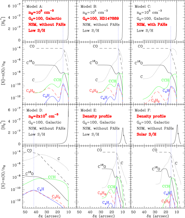
Figure 8: Predictions of the spatial variation of the abundance relative to H₂, using a unidimensional PDR code. For each model, the abundance of the population of the the upper level of the 2.12$\,\mathrm{\mu m}$ H₂ line (i.e. v=1, J=3), written $[$H${}_{2}^{\star}]$, is shown in linear scale (top). The C, CO and hydrocarbon abundances are shown in logarithmic scale (bottom). The modeled cloud is illuminated from the right–hand side. The $\delta x$–axis origin has been set so that $[$H${}_{2}^{\star}]$ peaks at the position of the observed H₂ peak (i.e. $\delta x=10^{\prime\prime}$). The vertical dotted blue line indicates the peak of the c-C₃H₂ and C₄H abundances. Each model is described in 3 lines: i) the density structure, ii) the UV–field properties and iii) the chemical network used. 6 different models are compared here. Our reference model is labeled A. The total hydrogen density is kept uniform at a value of $n_{\mathrm{H}}=10^{5}\,\mathrm{cm^{-3}}$. The far–UV intensity of the radiation field is G${}_{0}=100$ (in Draine units) and the extinction curve is the mean Galactic one. The chemical network rate file is the New Standard Model one with minor modifications described in the text. Charge exchange reactions between C⁺ and PAHs are not taken into account. The gaseous sulfur abundance is low compared to solar (i.e. S/H = $5.8\times 10^{-8}$). The parameters varied in other models are emphasized in red. Model B uses a different extinction curve. Model C adds reactions of charge exchange between C⁺ and PAHs. Model D decreases the uniform total hydrogen density. Models E and F use the density profile derived from the model of the H₂ observations (Habart et al. 2004, 2005). Model F uses a solar gaseous sulfur abundance (i.e. S/H = $10^{-5}$).

We have used a monodimensional PDR code (Le Petit et al. 2002, http://aristote.obspm.fr/MIS/) for modeling the observations of the Horsehead nebula. The slab geometry is locally appropriate as seen on Fig. 3. We did not take into account projection effects as the source is viewed almost edge-on. Indeed, Habart et al. (2005) show that the main effect of the PDR possible small inclination ($<6^{\circ}$) is to enlarge the peak profiles and to shift them all compared to the model edge. The model includes a detailed treatment of the photo–dissociation of H₂ and the CO isotopes as well as the statistical equilibrium of their rovibrational (rotational, respectively) states in a steady state approach. The parameters of the model include the elemental abundances, the cosmic ray ionization rate, the scaling factor of the interstellar ultraviolet radiation field (ISRF) measured in Draine units, the density profile and the grain parameters. As the observations involve complex carbon molecules, we have used the so called “new standard model” chemical rate file of Herbst and collaborators (Lee et al. 1998), available on the web site. In a previous paper (Teyssier et al. 2004), we have found that the other extensive chemical rate file provided by the UMIST group (Le Teuff et al. 2000) gave close results on the carbon chain molecules. As C¹⁸O observations are reported, we have added to this reaction set, the main isotopic molecules involving ¹⁸O and introduced the corresponding fractionation reactions (Graedel et al. 1982). We have also introduced the photo–dissociation rates given by van Dishoeck (1988), when available, which have been calculated specifically with the Draine ISRF and which were different from the values reported in the chemical rate file. The resulting chemical network involves about 450 chemical species and 5000 reactions. Only the most stable isomeric forms of hydrocarbons are considered here.

We define a reference model (hereafter named model A) of the Horsehead nebula as a uniform sheet of gas and dust of total hydrogen density $n_{\mathrm{H}}=10^{5}\,\mathrm{cm^{-3}}$ exposed to a ISRF of 100 measured in Draine units. The cosmic ray ionization rate has a value of $5\times 10^{-17}\leavevmode\nobreak\ \mbox{s}^{-1}$ and the elemental abundances are as follows: C/H = $1.38\times 10^{-4}$, O/H = $3.02\times 10^{-4}$, ¹⁸O/H = $6\times 10^{-7}$, N/H = $7.95\times 10^{-5}$, S/H = $5.8\times 10^{-8}$, Cl/H = $1.86\times 10^{-9}$, P/H = $9.3\times 10^{-10}$, Fe/H = $1.7\times 10^{-9}$, Mg/H = $10^{-8}$, Na/H = $2.3\times 10^{-9}$. The properties of the grains are the same as described in Le Petit et al. (2002), i.e. the size distribution law is taken from Mathis et al. (1977) with an exponent of $-3.5$ and we describe the attenuation of grains from the far–UV to the visible via the galactic extinction curve given as an analytic function of 1/$\lambda$ by including the coefficients derived by Fitzpatrick & Massa (1988). Charge exchange reactions between C⁺ and PAHs are not taken into account. The gas to dust mass ratio is 100.

Fig. 8 shows i) the abundance of the H₂ rovibrationnally excited in the v=1, J=3 level at the origin of the 2.12$\,\mathrm{\mu m}$ line (this abundance is hereafter referred to as $[$H${}_{2}^{\star}]$) and ii) the C, CO and hydrocarbon abundances for this reference model and 5 variants. We ensure that the $[$H${}_{2}^{\star}]$ peak position is set at $\delta x=10^{\prime\prime}$ as in the observations. Our reference model correctly reproduces the observed 3 to $5^{\prime\prime}$ offset between the hydrocarbon and H₂ peaks. The C¹⁸O also peaks behind the hydrocarbons at $\delta x=20-25^{\prime\prime}$. However, the H₂ profile is not correctly modeled here.

In model B, we replaced the Galactic extinction curve by one more representative of molecular gas. We have chosen HD 147889 in Ophiuchus. Its extinction curve has a rather strong far–UV rise ($E_{B-V}=1.09$ Fitzpatrick & Massa (1988)). Its ratio between the total and selective extinctions, $R_{V}$, is 4.2 a typical figure for molecular gas (Gordon et al. 2003; Cardelli et al. 1989). The PDR stratification does not qualitatively change compared to model A: It is just compressed. In model C, we added reactions of charge exchange between C⁺ and PAHs. This enhances the neutral atomic carbon abundance but does not have a large effect on the hydrocarbons: Only CCH peaks closer from the H₂ peak compared to model A. Neither model B nor C improves the modeling of the H₂ profile.

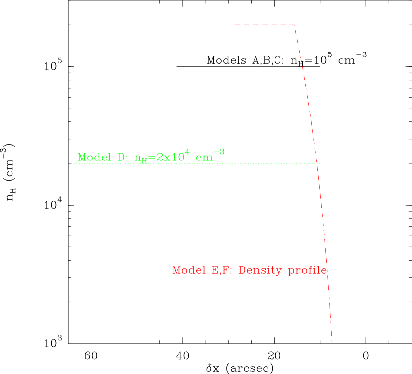
Figure 9: Spatial variation of the total hydrogen density in models A to F. In model E and F, the density is increasing as a power law of scaling exponent 4 on the first $10^{\prime\prime}$ and then is kept constant at a value of $2\times 10^{5}\,\mathrm{cm^{-3}}$. As in Fig. 8, the x-axis origin has been set so that $[$H${}_{2}^{\star}]$ peaks at the position of the observed 2.12$\,\mathrm{\mu m}$, H₂ line peak (i.e. $\delta x=10^{\prime\prime}$).

As shown by model D, E and F, the density structure has a major impact on the PDR structure. Fig. 9 shows the density profiles associated to each model. When keeping the total hydrogen density uniform but decreasing its value to $2\times 10^{4}\,\mathrm{cm^{-3}}$ (as in model D), the carbon and hydrocarbon abundance peaks highly broadened and shifted inward by more than $20^{\prime\prime}$, a prediction clearly violated by the high resolution PdBI data. Model E and F uses a density profile provided by Habart et al. (2004, 2005) to fit the 2.12$\,\mathrm{\mu m}$–H₂ emission. Indeed, the $[$H${}_{2}^{\star}]$ profile qualitatively changes (it is now a peak rising from zero at the PDR edge) but it also reproduces the H₂ filament width. Those two models which impose a steep total hydrogen density gradient at the PDR edge, are the only ones that succeed to correctly reproduce the offset between the hydrocarbon and H₂ peaks as well as the form of the H₂ peak. The sole difference between models E and F is the gaseous sulfur abundance: sulfur is depleted from the gas phase in model E (S/H = $5.8\times 10^{-8}$) while the gaseous sulfur abundance is solar in model F (S/H = $10^{-5}$).

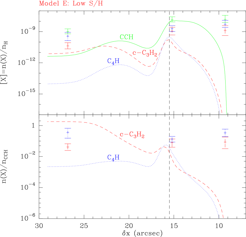
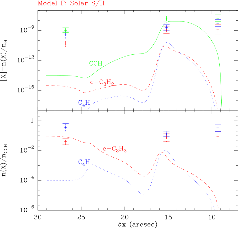
Figure 10: Comparison between our two best models (curves) and observed (points with error bars) abundances of the small hydrocarbons. CCH is shown as a green, plain line, c-C₃H₂ as a dashed, red line and C₄H as a blue dotted line. The top and bottom panels respectively show abundances relative to the total hydrogen density and CCH. The dashed vertical line shows the position where the total hydrogen density profile swaps from a steep gradient to a constant.

Fig. 10 is a zoom for our two best models (i.e. E and F) of the spatial variations of the abundances of hydrocarbons relative to i) total hydrogen density (top panel) and ii) CCH (bottom panel). The observed abundances are overplotted with their error bars. The dashed vertical line separates the zone where the proton gas density is constant from the zone where the proton gas density rapidly decreases outward. This latter zone is associated with the PDR. The sulfur elemental abundance has different effects in those two regions. In the region of moderate visual extinction (i.e. the“IR edge” and the “IR peak” where $A_{V}{}\la 1$), the charge transfer reaction between C⁺ and S leading to S⁺ and C reinforces the abundance of neutral carbon and thus enables the formation of carbon chains via the rapid neutral-carbon atom reactions. However this effect is small. Indeed this is in the dark region where the sulfur elemental abundance has a large effect. When the sulfur abundance is solar, the small carbon chains $\rm C_{2}$, CCH, $\rm C_{2}H_{2}$, $\rm C_{3}H$, $\rm C_{3}H_{2}$ and $\rm C_{4}H$ react with $\rm S^{+}$ to give $\rm C_{2}S^{+}$, $\rm CCS^{+}$, $\rm HC_{2}S^{+}$, $\rm C_{3}S^{+}$, $\rm HC_{3}S^{+}$ and $\rm C_{4}S^{+}$. In this main destruction path of the small carbon chains, one hydrogen atom is released impairing the reformation of the carbon chains. When S is higly depleted as in Model E, this destruction mechanisms is superseded by other paths involving $C^{+}$. Those paths form carbon chain ions which in turn contributes to the formation of other carbon chains. Overall, model E (i.e. low S/H) performs better in the comparison with observed abundances. The only exception is the $n(\mbox{c-C${}_{3}$H${}_{2}$})/n(\mbox{CCH})$ ratio at the “cloud” position. We will thus use model E only for comparison with the observations. At the IR peak (median point at $\delta x=15.5^{\prime\prime}$), CCH abundance is correctly reproduced while c-C₃H₂ and C₄H abundances are underestimated by at least a factor of 3. Discrepancies are much higher both at the “cloud” (point to the right at $\delta x=27^{\prime\prime}$) and the “IR edge” (point to the left at $\delta x=9^{\prime\prime}$) positions. In the UV–illuminated edge, the modeled $[\mbox{CCH}{}]$ has a quite shallow increase with $\delta x$ while the modeled $[\mbox{c-C${}_{3}$H${}_{2}$}]$ and $[\mbox{C${}_{4}$H}]$ share the same steep abundance profile. By contrast, the observed (“IR edge”) abundances are very similar for the 3 species, reflecting the very good spatial correlation between the different hydrocarbons (see Fig. 4). This discrepancy is independent of our knowledge of the total hydrogen density as it is also seen when comparing abundances relative to CCH.

In summary, none of our models is able to correctly reproduce the relative stratification of H₂ and small hydrocarbons. Comparison of model A and C shows that to reproduce the observed offset between hydrocarbon and H₂ peaks, we need a high total hydrogen density ($10^{5}\,\mathrm{cm^{-3}}$). By varying the profile density (model E and F), a shallow total hydrogen density increase at the PDR edge is needed for reproducing the profile of the 2.12$\,\mathrm{\mu m}$ H₂ line. However, the shallower the total hydrogen density increase, the larger the modeled offset between H₂ and the hydrocarbons. A good compromise is provided by a total hydrogen density profile increasing as a power law with a scaling exponent 4 on the first $10^{\prime\prime}$ and then constant at a value of $2\times 10^{5}\,\mathrm{cm^{-3}}$. Habart et al. (2005) shows that this model essentially correspond to a constant pressure model (with $P=4\times 10^{6}\,\mathrm{K\,km\,s^{-1}}$). Finally, model E with low sulfur elemental abundance performs better than model F with solar abundance. Nonetheless, even model E do not succeed to reproduce the good hydrocarbon correlation seen in the illuminated part of the PDR: while CCH is correctly predicted to have a smooth abundance increase, modeled c-C₃H₂ and C₄H abundances show a much too steep increase.

4.2 Can the fragmentation of PAHs contribute to the synthesis of small hydrocarbons?

Examining the model predictions in more details, three hypotheses can be proposed for explaining the discrepancies between model calculations and observations:

• The photo–dissociation rates used in the models may be incorrect. As the main destruction process near the cloud edge is photo–dissociation, the actual values of the photo–dissociation rates are critical for an accurate prediction. However, similar results are obtained with the UMIST95 and NSM rate files. The photo–dissociation rates for c-C₃H₂, C₃H and C₄H are 10^-9 s^-1 for both rate files, and differ by a factor of two for CCH (i.e. $0.51\times 10^{-9}$ s^-1 for UMIST95 and $10^{-9}$ s^-1 for NSM). The photo–dissociation rates of larger chains are similar. In most cases, except for CCH and acetylene, the numbers given in the rate files are not well documented. For instance, van Dishoeck (1988) discusses the photo–dissociation rate of c-C₃H₂ and concludes that it is accurate within an order of magnitude. More accurate photo–dissociation rates are clearly needed for the carbon chains and cycles. Recent calculations have been performed for C₄H showing that the photo–dissociation threshold is 5.74 eV, but that efficient photo–dissociation requires more energetic photons, typically above 6.5 eV (Graf et al. 2001). However, it is unlikely that the rates are low enough to explain the large discrepancies between the models and the data since these molecules are known to be sensitive to UV–radiation (Jackson et al. 1991; Song et al. 1994).

• Another possibility is that the chemical networks are missing important reactions for the synthesis of hydrocarbons. Neutral–neutral reactions are progressively included in the rate files, but still are much less numerous than ion–molecule reactions. It is now known that atomic carbon, diatomic carbon and CCH may react with hydrocarbons (Kaiser et al. 2003; Stahl et al. 2002; Mebel & Kaiser 2002). More work remains to be done. However, preliminary tests using a more extended data base of chemical reactions have not led to significant improvement.

• The excellent spatial correlation between the mid–IR emission due to PAHs and the distribution of carbon chains suggests a last hypothesis: the fragmentation of PAHs due to the intense far UV–radiation could seed the interstellar medium with a variety of carbon clusters, chains and rings (Scott et al. 1997; Verstraete et al. 2001; Le Page et al. 2003; Joblin 2003, and references therein). These species would then further react with gas phase species (C, C⁺, H, H₂, etc.) and participate in the synthesis of the observed hydrocarbons. Fuente et al. (2003) also favor this explanation for explaining the abundance of c-C₃H₂ they observed in other PDRs.

A correct exploration of this third hypothesis needs a good qualitative and quantitative description of both the fragmentation and reformation of PAHs, which is out of the scope of this paper. We here give only a few indications. Omont (1986) pioneered the attempts to understand the role of PAHs in the interstellar chemistry. Elaborating on this work, Lepp & Dalgarno (1988) suggested that participations of PAHs in the ion chemistry of dense clouds lead to large increase in the abundances of small hydrocarbons. Indeed, when the PAH fractional abundance exceeds $\sim 10^{-7}$, the formation of PAH^- triggers mutual neutralization of the positive atomic and molecular ions and introduces new pathways for the formation of complex molecules. The equilibrium abundances of neutral atomic carbon C, CCH and c-C₃H₂ may thus be enhanced by two order of magnitude. By comparison, our model C which includes charge exchange between C⁺ and PAHs, shows a decrease of C₄H and c-C₃H₂ abundances by at least an order of magnitude in the dark region. Introduction of mutual neutralization between C⁺ and PAH^- could be an interesting alternative to our “artificial” lowering of the sulfur abundance. We are currently acquiring CS data at PdBI to constrain the S chemistry independently.

Lepp et al. (1988) suggested that the ion chemistry of diffuse clouds has little impact on the CH, OH and HD abundance, but can lead to large increase in the abundance of other species (H₂, NH₃ and most noticeably $\rm CH_{4}$ and $\rm C_{2}H_{2}$) by successive reactions of PAH and PAH^- with carbon and hydrogen atoms. Talbi et al. (1993) suggested that Coulombic explosion of doubly ionized PAH could create c-C₃H₂ through the electronic dissociative recombination of $\rm C_{3}H_{3}^{+}$. Laboratory experiments by Jochims et al. (1994) suggested that PAHs with less than 30-40 carbon atoms will be UV–photodissociated in Hi regions while larger ones will be stable. Based on those results, models by Allain et al. (1996b, a) indicate that only PAHs with more than 50 carbon atoms survive the high UV radiation field of the diffuse interstellar medium, whereas smaller PAHs such as coronene or ovalene are destroyed by the loss of acetylenic groups. Destruction timescales are a few years for neutral species and typically five time shorter for the corresponding cations. All those reactions starts from neutral or cation PAHs. They will be in competition with charge exchange and mutual neutralization discussed above. Mutual neutralization has a maximal effect in the transition region where the gas is molecular but the electronic abundance is significant. This region corresponds more or less to the region of maximum emission from the PAHs or slightly deeper in the molecular cloud. All other cited reactions are more efficient toward the illuminated edge where PAHs are mainly neutral. Recently, Le Page et al. (2003) discussed the possibility of addition reactions with ionized carbon, starting from the high reaction rate between C⁺ and anthracene measured by Canosa et al. (1995). If similar reaction rates persist for heavier PAHs, addition reaction with carbon would be very efficient for counteracting the destruction by far–UV photons.

From the observational point of view, the mid–IR emission due to PAHs is extended in interstellar clouds. On the other hand, a detailed analysis of the mid and far–IR images obtained by IRAS led Boulanger et al. (1990) and Bernard et al. (1993) to conclude that PAHs disappear in the dense cold cloud interiors, probably because they coagulate and/or condense. Stepnik et al. (2003) describe a convincing case for such a process in a small filament of the Taurus cloud. Rapacioli et al. (2004) have found clear evidences for spatial variations of the aromatic infrared band profiles, likely due to the spatial variation of the nature of their carriers. A sophisticated analysis of ISOCAM-CVF data allow them to separate the mid–IR spectra of the ionized and neutral PAHs from the spectra of carbonaceous very small grains (possibly PAHs aggregates). The very small grains are located at a larger distance from the illuminating stars than the PAHs, lending support to the idea that PAHs are produced from the photo–evaporation of these very small grains. While more examples are needed for understanding the origin and fate of interstellar PAHs, it appears nonetheless that these macro molecules are released in the gas phase in the UV–illuminated regions of the interstellar medium, i.e. in the diffuse clouds, in PDRs, etc. In those regions, the destruction of the carbon skeleton is the main process limiting the smallest possible PAH size. It is likely that some carbon bearing molecules are released in the gas phase in the UV–illuminated regions, either as a secondary product of the evaporation of the dust particles giving rise to PAHs, or as products of the destruction of the PAH carbon skeleton.

5 Summary and Conclusions

We have presented maps of the edge of the Horsehead nebula in rotational lines of excited H₂, CO, C¹⁸O and simple hydrocarbon molecules, CCH, c-C₃H₂ and C₄H with $6^{\prime\prime}$ resolution. All the hydrocarbon maps are strikingly similar to each other, and to the mid–IR emission mapped by ISOCAM (Abergel et al. 2003) while we measured a 3 to $5^{\prime\prime}$ offset between the hydrocarbon and H₂ peaks. State-of-the-art chemical models fail to reproduce both the PDR hydrocarbon stratification and the absolute abundances of 2 over 3 observed hydrocarbons. We have examined three hypotheses for improving the models, and we conclude that the most likely explanation is we are witnessing the fragmentation of PAHs in the intense far–UV radiation due to $\sigma$Ori.

A detailed modeling of the chemistry including this new mechanism is beyond the scope of this paper. Indeed, such a modeling requires rates for both the growth (by addition of molecules or of carbon and hydrogen atoms) and the fragmentation of PAHs. This last item requires an accurate description of the fragmentation cascade of PAHs, in all their possible equilibrium states (ionized, neutral, partially or totally dehydrogenated, …). Laboratory experiments such as the ion cyclotronic resonance cell PIRENEA in Toulouse (Joblin 2003) are key instruments in this perspective. In addition, the rate files used by the model need to be updated, with a special mention on the photo–dissociation rates of the simple carbon chains. A critical review of the role of neutral–neutral reactions in interstellar chemistry is also warranted.