Extragalactic Cosmic Rays and Magnetic Fields:
Facts and Fiction

Abstract

A critical discussion of our knowledge about extragalactic cosmic rays and magnetic fields is attempted. What do we know for sure? What are our prejudices? How do we confront our models with the observations? How can we assess the uncertainties in our modeling and in our observations? Unfortunately, perfect answers to these questions can not be given. Instead, I describe efforts I am involved in to gain reliable information about relativistic particles and magnetic fields in extragalactic space.

I What do we know?

We know that cosmic rays and magnetic fields exist in clusters of galaxies for several reasons. First, in many galaxy clusters we observe the so-called cluster radio halos with a spatial distribution which is very similar to that of the intra-cluster gas observed in X-rays. These radio halos are produced by radio-synchrotron emitting relativistic electrons (cosmic ray electrons = CRe) spiraling in magnetic fields. We do not have direct evidence of cosmic ray protons (CRp) probably due to their much weaker radiative interactions. However, in our own Galaxy the CRp energy density outnumbers the CRe energy density by two orders of magnitude, which makes the assumption of a CRp population in galaxy clusters very plausible.

Second, the Faraday rotation of linearly polarized radio emission traversing the intra-cluster medium (ICM) proves independently the existence of intracluster magnetic fields. It has been debated, if the magnetic fields seen by the Faraday effect exist on cluster scales in the ICM, or in a mixing layer around the radio plasma which emits the polarized emission (Bicknell et al. 1990, Rudnick & Blundell 1990). However, there is no valid indication of a source local Faraday effect in the discussed cases (Enßlin et al. 2003), and the Faraday rotation signal excess of radio sources behind clusters compared to a field control sample strongly supports the existence of strong magnetic fields in the wider ICM (Clarke et al. 2001, Johnston-Hollitt & Ekers 2004). The detailed mapping of the Faraday effect of extended radio sources reveals that the ICM magnetic fields are turbulent, with power on a variety of scales, and with a power-spectrum which is Kolmogoroff-type (see Vogt & Enßlin, these proceedings). All these Faraday rotation measurements support magnetic field strengths of the order of several $\mu$G.

The existence of ICM magnetic fields and cosmic rays is not too surprising, since there are plenty of energy sources available, which could have contributed:

• cluster mergers: shock waves and turbulence (e.g., Miniati et al. 2000, 2001),

• active galactic nuclei (e.g., Enßlin et al. 1997, 1998),

• supernovae remnants (e.g., Völk et al. 1996),

• galactic wakes (e.g., Jaffe 1980, Roland 1981, Ruzmaikin et al. 1989),

• decaying/annihilating dark matter particles (e.g., Colafrancesco & Mele 2001, Boehm et al. 2004).

Furthermore, we have a basic understanding of relevant physical processes, such as

• particle cooling/radiation mechanisms,

• particle acceleration by shocks and turbulence,

• magneto-hydrodynamics.

In principle, we just have to put all these pieces together in order to get an understanding of magnetic fields and cosmic rays in galaxy clusters. This is done for the cosmic rays in a very schematic way in Fig. 1. The problem with such a generic approach is, that there are large uncertainties in the theoretical description of the different plasma processes which do not allow to decide a priori which are the dominant processes are within the complex network. Here, we will discuss two possibilities:

• the relativistic electrons seen in cluster radio halos are re-accelerated by cluster turbulence (e.g., Jaffe 1980, Roland 1981, Giovannini et al. 1993, Brunetti et al. 2001, 2004, Gitti et al. 2001)

• the radio emitting CRe are secondaries from hadronic interactions of a long-living CRp population within the ICM gas. (e.g., Dennison 1980, Vestrand 1982, Blasi & Colafrancesco 1999, Dolag & Enßlin 2000, Pfrommer & Enßlin 2004a)

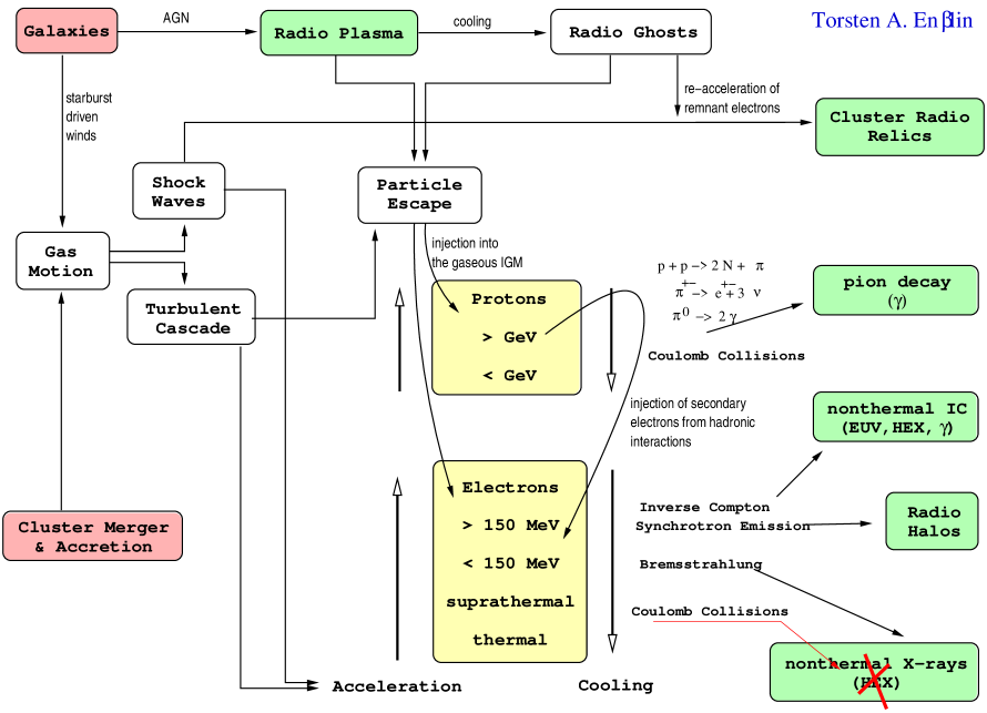
Fig. 1.—: Basic theory building blocks covering most of the proposed scenarios for the production and maintenance of relativistic particle populations in galaxy clusters and their observational consequences. Nearly all theoretical scenarios for cluster radio halos are summarized within this figure (e.g., re-acceleration model, hadronic model, hybrid hadronic-re-acceleration model, and many more). Red boxes: the main energy sources, yellow boxes: particle populations (CRp, CRe), green boxes: observables, white boxes: physical processes/phenomena which are (nearly) unobservable. The red cross indicates that the possibility that the reported non-thermal X-rays are generated by Bremsstrahlung of a super-thermal electron population runs into energetic problems due to strong Coulomb losses of such electrons (Petrosian 2001).

In order to have a chance to discriminate between the different theoretical models, detailed information on the electron spectrum would be very helpful, since the different scenarios exhibit different characteristics. An attempt to collect such information is displayed in Fig. 2. From the figure and the discussion in the caption it becomes clear that the interpretation of the Extreme Ultraviolet (EUV) and High Energy X-ray (HEX) flux reported for Coma as Inverse Compton scattered CMB photons would require magnetic fields of $1.4\,\mu$G (EUV) or significantly less (HEX). Such weak field strengths are an obvious contradiction to the Faraday method based estimates of several $\mu$G, especially if one compares magnetic energy densities or electron spectra as plotted in Fig. 2.

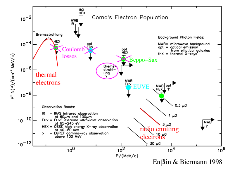
Fig. 2.—: Electron spectrum in the Coma cluster of galaxies (adopted from Enßlin & Biermann 1998). Red lines indicate parts of the electron spectrum we know to exist: thermal electrons (left), and radio-synchrotron electrons (right). The exact spectral location of the latter depends on the unknown ICM magnetic field strength. The upper limits result from physical processes, which would have produced photons in excess of observational constraints, if more than the indicated electrons of a given energy were present in the ICM. One process is Inverse Compton scattering of known background photon fields into observational bands. The other is Bremsstrahlung from energetic electrons with the ICM gas. Some of the used observations are actual claims of detections, and therfore could be measurements of the electron spectrum. Green points indicate possible explanations of the reported high energy X-ray (HEX) excess measured by Beppo-Sax (Fusco-Femiano et al. 1996, 2004, but see Rosetti & Molendi 2004, who do not find a significant signal). Blue points indicate possible explanations of the reported extreme ultraviolet excess measured by EUVE (e.g., Liu et al. 1996). However, some of the marked possibilities are unlikely (marked by pink crosses): severe Coulomb losses would remove super-thermal and mildly relativistic electron populations too quickly to be replenished (Petrosian 2001, Enßlin, Lieu, Biermann 1999). The IC scattering of optical photons into the HEX band would require too many relativistic electrons to be consistent with other upper limits resulting from Bremsstrahlung.

II What are our prejudices?

(a) Typical cluster magnetic field strength

Depending whom one asks, or which paper on cluster physics one consults, the assumption of the magnetic field strength differ significantly. Sub-micro-Gauss fields are assumed when an emphasize is given to the Inverse Compton scattering of CMB photons into the EUV and HEX energy bands. Super-micro-Gauss fields are assumed in the context of the interpretation of Faraday rotation signals.

Both methods of field estimates have their weak points. The inverse Compton argumentation can only provide strict lower limits to magnetic fields strength. The used observed EUV or HEX flux could have (partially) resulted from a different source or could be a measurement artefact. Therefore, the number of relativistic electrons could be smaller than assumed in the estimate, requiring stronger magnetic fields in order to provide the same amount of observed synchrotron emission.

Faraday rotation based field estimates are also not straightforward, since magnetic field reversals along the line of sight partially cancel each other’s Faraday signal. What is left as a typical cluster Faraday signal is the result of a random walk in rotation measure (RM) in the case of turbulent magnetic fields. The statistical RM signal depends on the statistical magnetic field strength times the square root of the magnetic autocorrelation length. The latter is unknown, and thus the Faraday based field estimates suffer from this uncertainty. However, the statistical properties of Faraday maps may allow to measure the magnetic autocorrelation length under relative reasonable assumptions of statistical isotropy and homogeneity of the magnetic fields (see Vogt & Enßlin, these proceedings).

It can be seen, that the Faraday rotation based field estimates can not be accommodated by sub-micro-Gauss field strength. For a typical cluster like Coma, $3-5\,\mu$G are reproducing the Faraday signal if a magnetic length-scale of 10 kpc is assumed. Lowering the magnetic field strength by one order of magnitude – as suggested by the IC based field estimates (in the case of the HEX excess) – would require an increase of the magnetic length scale to $\sim$ Mpc in order to reproduce the Faraday signal strength. But fields ordered on the cluster size would produce a nearly homogeneous RM signal, and not exhibit the many sign reversals observed in clusters.

(b) The origin of radio halos

Also the origin of the relativistic electrons producing the cluster radio halos is controversially debated. There are the re-acceleration models, which are favored by some authors since they are able to reproduce nearly every observational feature reported so far. And then there are the hadronic models, which are favored by others not only because of their simplicity, but also since the necessary cosmic ray proton population should be present in the ICM because most cosmic ray acceleration mechanisms are believed to preferentially accelerate protons.

III How to verify models?

It is often claimed that a model or theory is verified. However, theories can only be falsified. To be a scientific theory, it has to be falsifiable (Popper). This means, it must be possible to derive from it unambiguous predictions for doable experiments such that, were contrary results be found, at least one premise of the theory would have proven not to apply to nature.

Let us compare the different models for radio halos in the light of this statement:

(a) Hadronic model

The hadronic model is therefore a very good theory in the sense of Popper, since it makes a number of testable predictions.

1. The hadronic model predicts gamma and neutrino fluxes from clusters of galaxies.The gamma ray flux should be detectable with GLAST (Pfrommer & Enßlin and also Reimer, these proceedings),

2. The hadronic model can not explain very strong spectral bending in the radio, since even a mono-energetic proton population injects a broad electron spectrum, which produces an even broader synchrotron spectrum.

3. Furthermore, the necessary energy budget of the hadronic model can exceed the available energy sources, especially in the outer, low-density regions of clusters, where targets for an efficient CRp to CRe conversion are rare.

Some of these predictions seem to put already some stress on the hadronic model.

There is a strong spectral break reported for the total flux of the Coma cluster (Thierbach et al. 2003), which would be too strong for the hadronic model. Actually, this spectral break is too strong for any kind of synchrotron emission, indicating that there might be some problems with the spectral dataset of the Coma radio halo compiled from the literature. The strong spectral break might be partly explained by a contamination of the high frequency measurements by the Sunyaev-Zeldovich effect, however, it could also be an artefact of the very difficult radio astronomical measurement of extended radio halo luminosities in the vicinity of very strong point sources.

It was shown that at least the radio halos in the Coma and Perseus clusters do not violate the energy constraints (Pfrommer & Enßlin 2004b). In order to produce the observed radio emission without too much energy in CRp, the hadronic models favor larger magnetic field strength, in the range which are supported by the Faraday rotation measurements.

The prediction of gamma rays could have not been tested by existing telescope sensitivities. Future gamma ray telescopes have the potential to ultimately refute the hadronic model, since there is an unavoidable minimum gamma ray flux of the order of the total radio flux predicted for this class of models. If magnetic field strength are as low as $3\,\mu$G or less, the predicted gamma ray flux of the hadronic model has to be larger than this minimum prediction.

(b) Re-acceleration models

The re-acceleration model has not made unique predictions which have the potential to allow to refute the model observationally. The model seems to be able to fit any yet reported radio profile and spectra due to its many poorly constrained parameters. Therefore, distinctive predictions of the re-acceleration model would be very important, if they can be made at all (see Brunetti in these proceedings for first predictions of the re-acceleration model).

IV How to access uncertainties?

Reliable spectral information on radio halos has the potential to refute the hadronic model. However, there are many known, and maybe some unknown sources of artefacts in radio astronomy, which can perturb the measured spectrum. To understand the meaning and significance of features and spectra we need an end-to-end analysis of the data reduction process. This analysis should go from the detector signal, through (self)-calibration, to the map making, point source removal and halo flux integration step. Without such an analysis it would be premature to claim that the hadronic model is ruled out due to the reported spectral steepening of the Coma radio halo.

Also for the Faraday rotation measurements such an analysis would be highly desirable, in order to understand if and how observational artefacts influence our field estimates. In order to go into this direction, methods to quantify the level of noise and artefacts in Faraday maps were developed (Enßlin et al. 2003). They were used to verify the improved quality of Faraday maps and even the accuracy of Faraday error maps generated with the new Polarization Angle Correcting rotation Measure Analysis (PACMAN) algorithm (Dolag et al. 2004, Vogt et al. 2004). These maps were then analyzed with a maximum likelihood power spectrum estimator (Vogt & Enßlin, submitted), which is based on the cross correlation of Faraday signals in pixel pairs, as expected for a given magnetic power spectrum and galaxy cluster geometry (Enßlin & Vogt 2003, Vogt & Enßlin 2003).

The result of this exercise is not only a magnetic power spectrum, which is corrected for the complicated geometry of the used radio galaxy and of the Faraday screen, but also an assessment of the errors, and even the cross correlation of the errors. The power spectrum of the Hydra A cluster cool core region, which is displayed in Fig. 3, exhibits a Kolmogoroff-like power law on small scales, a concentration of magnetic power on a scale of 3 kpc (the magnetic auto-correlation length) and a total field strength of $7\pm 2\,\mu$G. The given error is the systematic error due to uncertainties in the Faraday screen geometry. The statistical error is lower by one order of magnitude.

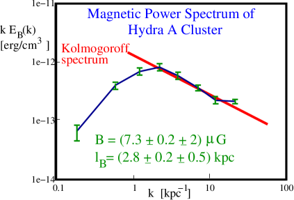
Fig. 3.—: Magnetic power spectrum within the cooling flow region of the Hydra A cluster of galaxies (for details see Vogt & Enßlin, these proceedings). The last data-point at large k-values is likely affected by map noise and should be discarded.

V Is a consistent picture possible?

(a) Combining observational information

Here, I am attempting to draw a consistent picture, which may explain at least a significant subset of the observational information:

• the Faraday rotation observations, which point towards turbulent fields strength of several $\mu$G strength: in the cool core region of the Hydra A cluster a field strength of 7$\mu$G correlated on 3 kpc; in non-cooling flow clusters like Coma somewhat lower fields (say 3$\mu$G) with a somewhat larger correlation length (say 10-30 kpc).

• the radio halo synchrotron emission of CRe in Coma

• the EUV excess of the Coma cluster, which may be understood as being inverse Compton scattered CMB light

The Faraday measurements provide us with volume averaged magnetic energy densities, since the RM dispersion scales as

$$\langle{\rm RM}^{2}\rangle\propto\langle B^{2}\rangle_{\rm Vol}.$$ (1)

The synchrotron emission is also (approximately) proportional to the magnetic energy density, but weighted with the CRe population around 10 GeV:

$$L_{\rm radio}\propto\langle B^{2}\,n_{\rm CRe}\rangle_{\rm Vol}.$$ (2)

Finally, the inverse Compton flux is a direct measurement of the number density of CRe (of the appropriate energy, see Fig. 2):

$$L_{\rm IC}\propto\langle n_{\rm CRe}\rangle_{\rm Vol}.$$ (3)

Combining the latter two measurements provides a magnetic field estimate (for a given or assumed electron spectral slope), which is weighted with the CRe density:

$$\langle B^{2}\rangle_{\rm CRe}=\frac{\langle B^{2}\,n_{\rm CRe}\rangle_{\rm Vol}}{\langle n_{\rm CRe}\rangle_{\rm Vol}}\propto\frac{L_{\rm radio}}{L_{\rm IC}}$$ (4)

(b) Reconciling the discrepant field estimates

The magnetic energy density derived from the combination of synchrotron and inverse Compton flux is at least one order of magnitude lower than the one derived from RM measurements. This discrepancy might be reconciled if there is a significant difference between volume and CRe weighted averages. This would require

1. an inhomogeneous magnetic energy distribution,

2. an inhomogeneous distribution of the CRe,

3. an anti-correlation between these two.

The required conditions could be generated if there are physical mechanisms which

• produce inhomogeneous or intermittent magnetic fields

• anti-correlate the CRe density with respect to the magnetic energy density.

A very natural physical mechanism, which could provide this anti-correlation is synchrotron cooling in inhomogeneous magnetic fields. In case of an injection rate of CRe which is un-correlated with the field strength, the equilibrium electron density is

$$n_{\rm CRe}\propto(B^{2}+B^{2}_{\rm CMB})^{-1},$$ (5)

where $B_{\rm CMB}\approx 3.2\mu$G describes the field strength equivalent to the CMB energy density.

For illustration, we assume that only a small fraction $f_{B}=0.1$ of the volume is significantly magnetized with a field strength of $10\,\mu$G, and the rest with only $1\,\mu$G. We will see later that $f_{B}=0.1$ may be a plausible number. The volume average would give $\langle B^{2}\rangle_{\rm Vol}^{1/2}=3.3\,\mu$G, whereas the CRe average gives $\langle B^{2}\rangle_{\rm CRe}^{1/2}=1.5\,\mu$G. These numbers are in good agreement with the corresponding field estimates for the Coma cluster based on Faraday rotation and IC/synchrotron measurements, respectively. A larger ratio in magnetic field estimates could even be accomodated since the EUV emitting electrons are at energies below the synchrotron electrons. A spectral bump of an old accumulated electron population at these energies is therefore possible, and even plausible due to the minimum in the electron cooling rate at these energies.

The hadronic model would provide a CRe injection rate which is not correlated with the magnetic field strength, as would be required by the above explanation of the discrepancy of magnetic field estimates by the two methods would work. In contrast to this, in the re-acceleration model one would expect a strong positive correlation of CRe and magnetic field strength, since magnetic fields are essential for the CRe acceleration.

(c) Turbulent magnetic dynamo theory

It remains to be shown that there is also a natural mechanism producing intermittent magnetic fields. The Kolmogoroff-like magnetic power spectrum in the cool core of the Hydra A cluster indicates that the magnetic fields are shaped and probably amplified by hydrodynamical turbulence (e.g., De Young 1992). Therefore, we have to look into the predictions of the theories of turbulent dynamo theories.

It is generally found by a number of researchers that the non-helical turbulent dynamo saturates in a state with a characteristic magnetic field spectrum (e.g., Ruzmaikin et al. 1989, Sokolov et al. 1990, Subramanian 1999 and many others). The effective magnetic Reynolds number (including turbulent diffusion) reaches a critical value of $R_{\rm c}\approx$ 20 … 60. The magnetic fields should exhibit – more or less pronounced – the following properties:

• The average magnetic energy density $\varepsilon_{B}$ is lower than the turbulent kinetic energy density $\varepsilon_{\rm kin}$ by $\varepsilon_{B}\approx\varepsilon_{\rm kin}\,R_{\rm c}^{-1}$.

• The magnetic fluctuations are concentrated on a scale $l$, which is smaller than the hydrodynamical turbulence injection scale $L$ by $l\approx LR_{\rm c}^{-1/2}$.

• Correlations exist up to scale $L$, turn there into an anti-correlation, and quickly decay on larger scales.

• This may be understood by Zeldovich’s flux rope model, in which magnetic ropes with diameter $l$ are bent on scales of the order $L$.

• Within flux ropes, magnetic fields can be in equipartition with the average turbulent kinetic energy density.

• The magnetic drag of such ropes produces a hydrodynamical viscosity on large scales, which is of the order of $4\%$ of the turbulent diffusivity (Longcope et al. 2003).

(d) Confronting theory with observations

Turbulent magnetic dynamo theory predicts intermittent magnetic fields, as favored by the proposed explanation of the discrepancy in the different magnetic field estimate methods. Let’s see if the other predictions of the theory are in agreement with observations. We assume, that $R_{\rm c}$ is in the range 20 to 60.

• The expected turbulent energy density in the Hydra A cluster core is of the order of $(0.3\ldots 1)\,10^{-10}\,{\rm erg\,cm^{-3}}$, which corresponds to turbulent velocities of $v_{\rm turb}\approx(300\ldots 500)\,{\rm km/s}$. This is comparable to velocities of buoyant radio plasma bubbles (Enßlin & Heinz 2002), which are expected to stir up turbulence (e.g., Churazov et al. 2001).

• The expected turbulence injection scale in the Hydra A cluster core is of the order of $(15\ldots 25)$ kpc, again consistent with the radio plasma of Hydra A being the source of turbulence. The dynamical connection of the radio source length scale and the magnetic turbulence scale would explain why the Faraday map of Hydra A is conveniently sized to show us the peak of the magnetic power spectrum.

• This prediction is hard to test since fluctuations on scales larger than the radio source are not measurable due to the limited RM map size. However, the downturn of the magnetic power spectrum at small $k$-values is at least in agreement with this prediction.

• Magnetic intermittency in form of flux ropes might have been detected as stripy patterns in the RM map of 3C465 (Eilek & Owen 2002).

• The fraction of strongly magnetized volume can become as small as $f_{\rm B}=R_{\rm c}^{-1}\approx 0.02...0.05$, a value which is more extreme than what we assumed in our example for the Coma cluster.

• The expected hydrodynamical viscosity on large scales in the Hydra cluster is of the order of $(1\ldots 4)\,10^{28}\,{\rm cm^{2}/s}$. It is interesting to note, that a lower limit on the large scale viscosity of the comparable Perseus cluster cool core of $4\cdot 10^{27}\,{\rm cm^{2}/s}$ was estimated by Fabian et al. (2003). An upper limit on the viscosity in the (somewhat different) Coma cluster of $\sim 3\cdot\,10^{29}\,{\rm cm^{2}/s}$ was derived by Schücker et al. (2004). Both limits are consistent with our coarse estimate of the large scale viscosity and enclose it.

VI Conclusion

To summarize, it is not clear if all observational information can be fitted into a single consistent picture of extragalactic cosmic rays and magnetic fields. It might be that we have to revise some of our data-points. The choice of data-points which were used (or ignored) here for the construction of the presented physical picture reflects the author’s personal prejudices and may certainly be questioned.

Nevertheless, it should have become clear that the existence of strong and possibly intermittent magnetic fields (several $\mu$G) in galaxy clusters is strongly supported by the recent detection of a Kolmogoroff-like magnetic power spectra in the Hydra A cluster. Some of the discrepancies between Faraday-based and inverse Compton-based field estimates can be explained by effects caused by magnetic intermittence, which is expected from turbulent dynamo theory.

Furthermore, it is argued that the hadronic generation mechanism of the cluster radio halo emitting electrons is a viable model. This model is providing a number of stringent predictions (like minimal gamma ray fluxes, limits on spectral bending, maximal possible radio luminosities), which allows detailed consistency tests with future sensitive measurements. The fact that this class of models seems to be more under pressure by some reported observations compared to alternatives as the also viable re-acceleration model may be caused by the larger number of predictions of the hadronic model in conjunction with underestimated systematic observational errors.

ACKNOWLEDGEMENTS It is a pleasure to thank the conference organizers for the excellent meeting, and the very warm hospitality. I also want to thank Corina Vogt and Christoph Pfrommer for discussion and comments on the manuscript

REFERENCES

Bicknell, G. V., Cameron, R. A., Gingold, R. A., 1990, ApJ 357, 373

Blasi, P., Colafrancesco, S., 1999, Astroparticle Physics 12, 169

Boehm, C., Enßlin, T. A., Silk, J., 2004, Journal of Physics G Nuclear Physics 30, 279

Brunetti, G., Blasi, P., Cassano, R., Gabici, S., 2004, MNRAS 350, 1174

Brunetti, G., Setti, G., Feretti, L., Giovannini, G., 2001, MNRAS 320, 365

Churazov, E., Brüggen, M., Kaiser, C. R., Böhringer, H., and Forman, W., 2001, ApJ 554, 261

Clarke, T. E., Kronberg, P. P., Böhringer, H., 2001, ApJ 547, L111

Colafrancesco, S., Mele, B., 2001, ApJ 562, 24

De Young, D. S., 1992, ApJ 386, 464

Dennison, B., 1980, ApJ 239, L93

Dolag, K., Enßlin, T. A., 2000, A&A 362, 151

Dolag, K., Vogt, C., Enßlin, T. A., 2004, astro-ph/041214

Eilek, J. A., Owen, F. N., 2002, ApJ 567, 202

Enßlin, T. A., Biermann, P. L., 1998, A&A 330, 90

Enßlin, T. A., Biermann, P. L., Kronberg, P. P., Wu, X.-P., 1997, ApJ 477, 560

Enßlin, T. A., Heinz, S., 2002, A&A 384, L27

Enßlin, T. A., Lieu, R., Biermann, P. L., 1999, A&A 344, 409

Enßlin, T. A., Vogt, C., 2003, A&A 401, 835

Enßlin, T. A., Vogt, C., Clarke, T. E., Taylor, G. B., 2003, ApJ 597, 870

Enßlin, T. A., Wang, Y., Nath, B. B., Biermann, P. L., 1998, A&A 333, L47

Fabian, A. C., Sanders, J. S., Crawford, C. S., Conselice, C. J., Gallagher, J. S., Wyse, R. F. G., 2003, MNRAS 344, L48

Fusco-Femiano, R., dal Fiume, D., Feretti, L., Giovannini, G., Grandi, P., Matt, G., Molendi, S., Santangelo, A., 1999, ApJ 513, L21

Fusco-Femiano, R., Orlandini, M., Brunetti, G., Feretti, L., Giovannini, G., Grandi, P., Setti, G., 2004, ApJ 602, L73

Giovannini, G., Feretti, L., Venturi, T., Kim, K. T., Kronberg, P. P., 1993, ApJ 406, 399

Gitti, M., Brunetti, G., Setti, G., 2002, A&A 386, 456

Jaffe, W., 1980, ApJ 241, 925

Johnston-Hollitt, M., Ekers, R. D., 2004, astro-ph/0411045

Lieu, R., Mittaz, J. P. D., Bowyer, S., Breen, J. O., Lockman, F. J., Murphy, E. M., Hwang, C. ., 1996, Science 274, 1335

Longcope, D. W., McLeish, T. C. B., & Fisher, G. H. 2003, ApJ, 599, 661

Miniati, F., Jones, T. W., Kang, H., Ryu, D., 2001, ApJ 562, 233

Miniati, F., Ryu, D., Kang, H., Jones, T. W., Cen, R., and Ostriker, J. P., 2000, ApJ 542, 608

Petrosian, V. ., 2001, ApJ 557, 560

Pfrommer, C., Enßlin, T. A., 2004a, A&A 413, 17

Pfrommer, C., Enßlin, T. A., 2004b, MNRAS 352, 76

Roland, J., 1981, A&A 93, 407

Rossetti, M., Molendi, S., 2004, A&A 414, L41

Rudnick, L., Blundell, K. M., 2003, ApJ 588, 143

Ruzmaikin, A., Sokolov, D., Shukurov, A., 1989, MNRAS 241, 1

Schuecker, P., Finoguenov, A., Miniati, F., Böhringer, H., and Briel, U. G., 2004, A&A 426, 387

Sokolov, D. D., Ruzmaikin, A. A., Shukurov, A., 1990, in IAU Symp. 140: Galactic and Intergalactic Magnetic Fields, pp 499–502

Subramanian, K., 1999, Physical Review Letters 83, 2957

Thierbach, M., Klein, U., Wielebinski, R., 2003, A&A 397, 53

Vestrand, W. T., 1982, AJ 87, 1266

Vogt, C., Dolag, K., Enßlin, T. A., 2004, astro-ph/041216

Vogt, C., Enßlin, T. A., 2003, A&A 412, 373

Völk, H. J., Aharonian, F. A., Breitschwerdt, D., 1996, Space Science Reviews 75, 279