A High-Resolution Stellar Library for Evolutionary Population Synthesis

Abstract

We present a library of 1654 high-resolution stellar spectra, with a sampling of 0.3 Å and covering the wavelength range from 3000 to 7000 Å. The library was computed with the latest improvements in stellar atmospheres, incorporating non-LTE line-blanketed models for hot, massive (T_eff $\geq$ 27500 K) and line-blanketed models for cool (3000 K $\leq$ T_eff $\leq$ 4500 K) stars. The total coverage of the grid is 3000 K $\leq$ T_eff $\leq$ 55000 K and –0.5 $\leq$ log g $\leq$ 5.5, for four chemical abundance values: twice solar, solar, half solar and 1/10 solar. Evolutionary synthesis models using this library are presented in a companion paper. We tested the general behavior of the library by calculating and comparing equivalent widths of numerous H and HeI lines, and some of the commonly used metallic indices. We also compared the library with the empirical libraries STELIB and Indo-US. The full set of the synthetic stellar spectra is available from our websites (http://www.iaa.csic.es/$\sim$rosa and http://www.astro.iag.usp.br/$\sim$lucimara/library.html).

1 Introduction

Stars are the main energy source in normal galaxies. Their features are detected not only in the absorption-line spectra of normal, non-active galaxies, but also in starburst and HII galaxies, where emission lines usually dominate. Even in active galactic nuclei (AGNs), whose main energy source is gravity rather than nucleosynthesis, it has become evident that a significant component of the overall energy balance is stellar ionizing radiation (González Delgado, Heckman, & Leitherer 2001, and references therein). Analyzing the complex spectra of such galaxies and disentangling the individual ionizing sources is a major theme of contemporary astrophysics and cosmology. Key parameters such as, e.g., metallicity, age, or star-formation history allow us to understand how such galaxies form and evolve (Kauffmann et al. 2003a).

Over the past years, the quality of observations, both in terms of signal-to-noise and spectral resolution underwent a dramatic improvement. Progress has been made in the observations of galaxies themselves, but also with respect to data of suitable template stars (Le Borgne et al. 2003). The latter aspect is often not fully appreciated, but is nevertheless crucial for modeling any galaxy with spectral synthesis techniques. Large telescopes with high-resolution spectrographs and digital detectors have made it possible to obtain stellar spectra with a resolving power of 10⁵ and sub-percent noise levels for stars down to the limit of the Henry Draper catalog.

This progress has dramatically impacted evolutionary synthesis techniques. Such models describe the spectral and chemical evolution of stellar systems in an attempt to derive the properties of a stellar population in both nearby and distant galaxies (Tinsley 1980). Taking the star-formation history of the population (age, initial mass function [IMF], and star formation rate) as a free parameter, this technique minimizes the difference between observations and models and considers the best-fit solution as the true representation of the observations.

In the past, an analysis of stellar populations has often relied on equivalent widths of spectral features, discarding a huge part of the rich information present in modern spectra. An example are the widely used Lick indices which can be compared to selected features in narrow spectral windows (e.g., Worthey et al. 1994). While this technique is still our fundamental key to understanding the stellar content of most extragalactic systems (e.g., Trager 2004), global synthesis methods fitting the entire spectrum simultaneously are beginning to become feasible. An example is the modeling of 10⁵ nearby galaxies from the Sloan Digital Sky Survey by Kauffmann et al. (2003a).

The main challenge of this method is the need of a suitable library of stellar energy distributions (SEDs) at high spectral resolution. The available atlases in the literature have only intermediate or low spectral resolution (e.g., Jacoby, Hunter, & Christian 1984; Burstein et al. 1984; Walborn & Fitzpatrick 1990; Cananzi, Augarde, & Lequeux 1993). Alternatively, those libraries offering high spectral resolution are often limited to a small window of the full spectral range (Cenarro et al. 2001). Impressive improvement over previous observational atlases is the work of Le Borgne et al. (2003) and Valdes et al. (2004). However, the resolution is still only 3 Å or worse, or these libraries lack completeness in some important stellar evolutionary phases. The major limitation of all currently available high-resolution empirical libraries is the parameter space coverage. A particular concern are chemical abundances. Not only are we confined to observations of stars whose heavy-element content is often not much different from that of the Sun, but even worse, those stars have the chemical evolution of the Galaxy or the Magellanic Cloud imprinted in their spectra. Anomalous line strengths due to particular chemical histories have been suggested to account for discrepancies between observed and synthetic population spectra based on empirical templates (Maraston & Thomas 2000).

Theoretical stellar spectra do not suffer from this shortcoming. They can be calculated for any desired stellar type, luminosity class, chemical abundance, and wavelength range. Another important advantage of theoretical models is the knowledge of the continuum location: placing the continuum in observed spectra can never be done in an unbiased way because the location of the true continuum is unknown. Models predict both the line and the continuum spectrum, and the difference between the two allows an estimate of the severity of line blanketing. Theoretical libraries are already available in the literature, such as, e.g., ATLAS9 (Kurucz 1993b), one of the most widely used sets of stellar model spectra. One of the major drawbacks of this library is its very low resolution, a shortcoming recently improved by Murphy & Meiksin (2004). Another concern with Kurucz models is local thermodynamic equilibrium (LTE), which is not appropriate for hot stars. González Delgado & Leitherer (1999) avoided this problem by creating a high-resolution synthetic library at solar chemical abundance using a set of non-LTE models developed by Hubeny and collaborators (Hubeny 1998; Hubeny, Lanz, & Jeffrey 1995). However, computational restrictions limited the spectra to small spectral ranges around the most important Balmer and HeI lines.

Motivated by recent progress in atmosphere modeling, we have embarked on a project to compute a comprehensive set of stellar atmosphere models for implementation in the evolutionary synthesis codes Starburst99 (Leitherer et al. 1999) and sed@. In the present paper we discuss the choice of the model atmospheres and their main characteristics. An accompanying paper (González Delgado et al. 2004, hereafter GD04) provides a parameter study of the stellar population properties computed with the new model atmospheres.

This paper is organized as follows: In §2 we perform a trade study of the various model atmospheres and spectrum synthesis codes in the literature. In §3 we discuss the generation of the spectral library with particular emphasis on the parameter region where the predictions of different models overlap. The major trends of important spectral diagnostics with temperature, gravity, and chemical abundance are presented in §4. In §5 we test our theoretical spectra by comparing them to high-quality observations of standard stars. Finally, our conclusions are in §6.

2 Theoretical Models

2.1 Model atmospheres

Despite significant improvements over the past years, model atmospheres are far from perfect in reproducing real stars and still have serious limitations. Different codes are often optimized for a certain range of parameters (T_eff, log g, etc.), and not valid for others. Therefore it is necessary to understand the approximations and applicability limits made by each code in order to be able to choose between models for different types of stars. In this section we discuss the codes available in the literature and justify our preference for this work.

The vast majority of model atmospheres are 1D, time independent and hydrostatic, assume LTE and treat convection with a rudimentary mixing length. Every one-dimensional mixing-length convective model is based on the assumption that the convective structure averages out so that the emergent radiation depends only on a one-dimensional temperature distribution, something that is not always true. Furthermore, spectral line formation often occurs as a non-equilibrium process: under typical atmosphere conditions, radiative rates can dominate over collisional rates, and the radiation field departs from the Planck function. Non-LTE line formation is therefore neither special nor unusual, while LTE line formation is: LTE is an extreme assumption, not a cautious middle-ground. In general, non-LTE effects become progressively worse for higher temperatures (higher energy) or very low temperatures (fewer e^-), lower surface gravities (fewer collisions) and lower [Fe/H] (fewer e^- collisions and stronger UV radiation field) (Asplund 2003).

The microturbulent velocity is another problematic parameter that is not calculated self-consistently, except in the Sun. Usually it is treated as the parameter that minimizes the scatter among lines of the same ion in abundance analyses. It is known that the microturbulent velocity varies with the optical depth and that the opacity is strongly depend on microturbulent velocity. Models usually assume an average value.

Despite these complications, it is often possible to compute a model that matches the observed energy distribution and line spectrum of a star. However, to obtain the match it is necessary to adjust a number of free parameters: chemical abundance, effective temperature, surface gravity, microturbulent velocity, and the mixing length-to-scale-height-ratio in one-dimensional convective treatment.

One of the most widely used libraries is based on Kurucz’s (1993b) ATLAS9 model atmospheres. Kurucz models use the distribution function and line opacity computed by Kurucz (1979a,b) from the line data of Kurucz and Peytremann (1975). The latter authors computed gf-values for 1.7 million atomic lines for sequences up to nickel. That line list has provided the basic data and has since been combined with a list of additional lines, corrections, and deletions. Kurucz models incorporate line lists for the diatomic molecules H₂, CO, CH, NH, OH, MgH, SiH, CN, C₂ and TiO. In addition to lines between levels, these lists include lines whose wavelengths are predicted and are not good enough for detailed spectrum comparisons but are quite adequate for statistical opacities. Kurucz recomputed the opacities using these atomic and molecular data. Kurucz models are not adequate for M stars (T_eff $\leq$ 4000 K), because they lack line lists or opacities for triatomic molecules (Kurucz 1992).

Kurucz models follow from the classical approximations of steady-state, homogeneous, LTE, plane-parallel layers that extend vertically through the region where the lines are formed. In stars later than mid-A, convection can have a significant effect, therefore models cooler than 9000 K are convective. The mixing length theory was introduced in ATLAS6 (Kurucz 1979b). This theory is a phenomenological approach to convection in which it is assumed that one eddy (“bubble”) of a given size as a function of local mixing length transports all the convective energy. One of the shortcomings is the existence of an adjustable parameter $\alpha$, the scale height that a hot bubble rises in the atmosphere before dissipating its heat to the surrounding gas. The preferred value of $\alpha$ has changed with different ATLAS versions. In ATLAS9, $\alpha$ is assumed to be 1.25 to fit the energy distribution from the center of the Sun. However, the parameter $\alpha$ has to be set at different values to fit different types of observations (Steffen & Ludwig 1999), and no single value works well in all cases.

In ATLAS9, a horizontally averaged opacity and an “approximate overshooting” were included. This approximate overshooting is based on smoothing the convective flux over a certain fraction of the local pressure scale height at the transition between stable and unstable stratification (Castelli 1999). It yields a positive mean convective flux right at the beginning of the stable stratification. However, the treatment of convection is still approximate and may be a source of systematic errors (Gardiner, Kupka, & Smalley 1999). Gardiner et al. suggested that the mixing length approximation without overshooting works better for stars between 6000 K and 9000 K. They also found that different values of $\alpha$ are necessary for stars in different temperature ranges ($\alpha$ = 1.25 for 6000 K $\leq$ T_eff $\leq$ 7000 K, whereas $\alpha$ = 0.5 for T_eff $\geq$ 7000 K and T_eff $\leq$ 6000 K).

Kurucz models also fail where non-LTE and sphericity effects are important. Non-LTE effects are much stronger for higher temperatures (O and B stars) and for low gravities at any temperature (supergiants). A widely used model atmosphere that takes into account non-LTE is TLUSTY (Hubeny 1988; Hubeny & Lanz 1995; Lanz & Hubeny 2003). TLUSTY calculates a plane-parallel, horizontally homogeneous model atmosphere in radiative and hydrostatic equilibrium. The program allows departures from LTE and metal line blanketing, using the hybrid complete linearization and accelerated lambda iteration (CL/ALI) method (Hubeny & Lanz 1995). These models incorporate about 100000 non-LTE atomic levels and the blanketing effect of millions of Fe and Ni lines. A total of 8000 lines of the light elements are included, as well as 12 million lines from Fe III-VI and Ni III–IV. The opacity and radiation field are represented with an opacity sampling technique. The convection is treated with the mixing length theory. TLUSTY does not account for spherical geometry, which can be important in OB and Wolf-Rayet stars with strong winds (Aufdenberg et al. 1998, 1999).

A non-LTE code that takes into account stellar winds is WMBasic (Pauldrach et al. 1998, Pauldrach, Hoffmann, & Lennon 2001). This code calculates expanding atmospheres, taking into account line blocking and blanketing. The atomic data allow a detailed multilevel non-LTE treatment of the metal ions (C to Zn) and an adequate representation of line blocking and the radiative line acceleration. These models also include EUV and X-ray radiation produced by the cooling zones which originate from the simulation of shock heated matter.

Phoenix (Hauschildt et al. 1996) is a multi-purpose stellar atmosphere code for plane-parallel and spherical models. The original versions of Phoenix were developed for the modeling of novae and supernova ejecta (Hauschildt & Baron 1999 and references therein). Its more recent application to brown dwarfs is described in detail by Allard & Hauschildt (1995) and Hauschildt, Allard, & Baron (1999), and has served to generate grids of stellar model atmospheres that successfully described low-mass stars in globular clusters (Baraffe et al. 1995, 1997) and the Galactic disk main sequence (Baraffe et al. 1998).

The equilibrium of Phoenix is solved simultaneously for 40 elements, with usually two to six ionization stages per element and 600 relevant molecular species for oxygen-rich ideal gas compositions. The chemistry has been gradually updated with additional molecular species since Allard & Hauschildt (1995), using the polynomial partition functions of Irwin (1998) and Sharp & Huebner (1990). The H₃⁺ and H₂⁺ ions have been added to the chemical equilibrium and opacity database by using the partition function of Neale & Tennyson (1995) and a list of 3 $\times$ 10⁶ transitions by Neale, Miller, & Tennyson (1996). Van der Waals pressure broadening of the atomic and molecular lines is applied as described by Schweitzer et al. (1996). Dust is allowed to form, but assumed to dissipate immediately after formation (Allard et al. 2001). The convective mixing is treated according to the mixing-length theory. Both atomic and molecular lines are treated with a direct opacity sampling method.

2.2 The spectrum synthesis codes

It is important to distinguish between a atmosphere model and a profile synthesis model. A classical model atmosphere provides the run of temperature, gas, electron and radiation pressure, convective velocity and flux, and more generally, of all relevant quantities as a function of some depth variable (geometrical, or optical depth at some special frequency, or column mass). For comparison with observations, it is necessary to calculate the synthetic line spectrum from these models with a profile synthesis code. The synthetic spectrum quality will depend on the quality and adequacy of the atmosphere model, but also on the details of the line list adopted. Several codes are available in the literature for this task.

SYNTHE (Kurucz & Avrett 1981) is a spectrum synthesis program created by Kurucz to generate the surface flux for the converged model atmospheres from CD-ROMs 1 and 15 (Kurucz 1993a,c). The spectrum is computed in short intervals, typically at a resolving power of 500,000. Rotationally broadened spectra are computed for a number of values of vsin i, still at the same resolving power.

SYNSPEC (Hubeny et al. 1995) is a general spectrum synthesis program. It requires a model atmosphere as input. The program reads a general line list and dynamically selects lines which contribute to the total opacity, based on physical parameters of the actual model atmosphere. SYNSPEC then solves the radiative transfer equation, wavelength by wavelength in a specified spectral range, with a specified wavelength resolution. The wavelength points are not equidistant. Instead, they are calculated by the program in such a way that there is always a wavelength point at a line center, and in the midpoint between two neighboring lines. The program then adds a certain number of points equidistantly spaced between these two, such that the interval between the points does not exceed some specified value. This procedure assures that neither any line center nor any continuum window is omitted. The adopted continuum as well as the line opacity is fully specified by the user. In principle, the line and continuum opacity sources used in calculating a model stellar atmosphere and in calculating detailed spectrum should be identical, but due to practical limitations, they are usually not.

SPECTRUM (Gray & Corbally 1994) is another routine that computes synthetic spectrum in LTE, given a stellar atmosphere model. It treats each transition as a pure absorption line. The code is distributed with an atomic and molecular line list for the optical spectral region, suitable for computing synthetic spectra for temperatures between 4500 K and 20000 K. SPECTRUM does not compute adequate spectra for stars in which a significant part of the line formation occurs in the chromosphere or in stellar winds. These effects begin to become important in the Sun and cooler stars. SPECTRUM currently supports the following diatomic molecules: CH, NH, OH, MgH, SiH, CaH, SiO, C₂, CN, and TiO.

There are other codes described in the literature, but they are not suitable for generating a spectral library containing hundreds of model spectra with full Hertzprung-Russell diagram (HRD) coverage. Routines like MOOG (Sneden 1973) and SME (Valenti & Piskunov 1996) also generate spectral profiles, but their main purpose is to determine physical parameters of observed spectra by fitting line profiles. Owing to this requirements, they are optimized to generate profiles over very short wavelength ranges, and are not suitable for generating a library as we desire it.

2.3 Population synthesis code

Ideally, one would like to generate a stellar library using model atmospheres and model spectra that account for all the discussed effects across the full HRD: non-LTE, line-blanketing, sphericity, expansion, non-radiative heating, convection, etc. Clearly such an approach is unfeasible – even if the astrophysical models were available. The alternative, pragmatic method is to first identify the relevant temperature and gravity ranges that contribute to the spectrum of a population as predicted by a population synthesis code and then apply the best physics to those phases that matter the most.

We implemented this library into two stellar population synthesis codes: Starburst99 and sed@. The synthesis is done in two steps. First, the code computes the population of stars as a function of IMF and age. Then the line profiles of the population are synthesized by adding the luminosity-weighted spectra of individual stars. By restricting the synthesized spectrum to wavelengths longward of the space-ultraviolet, we avoid the domain where stellar-wind effects can dominate in hot massive stars. A spectrum of a young population generated with Starburst99 displays strong stellar-wind lines of, e.g., CIV and SiIV (Leitherer, Robert, & Heckman 1995). A code such as WMBasic would be required for the calculations of these profiles. On the other hand, a population older than $\sim$5 Myr shows few strong wind lines in the optical, and plane-parallel, static models are adequate in the OB-star regime. Consequently, TLUSTY models are an excellent choice, except for extremely wind-sensitive lines such as H$\alpha$ or HeII $\lambda$4686.

At the opposite extreme of the temperature range, line-blanketing becomes the dominant issue, and we should strive to apply the best possible physics to address blanketing. The spherical, fully blanketed Phoenix atmospheres are the models of choice for cool stars. Late-type stars become noticeable in the spectra of a stellar population at wavelengths longward of $\sim$5000 Å even at young ($\sim$10 Myr) ages, and their influence becomes progressively stronger at older ages and longer wavelengths.

While stars at the extreme end of the observed temperature range usually will not dominate the total optical light of a stellar population, they will contribute with some spectral lines detectable in the spectrum (at least in the populations relevant for this paper). Since observed and synthetic galaxy spectra are often compared with automatic least-square methods, missing even a few of such spectral lines may have rather significant consequences. Therefore, our rules for selecting the most appropriate atmospheric and profile models for implementation in our evolutionary synthesis codes are as follows:

(i) Line-blanketing must be accounted for at any position in the HRD.

(ii) Non-LTE is most significant at high temperatures.

(iii) Completeness of line lists is important for intermediate-type and paramount for cool stars.

This leads us to rely on TLUSTY for O stars, Phoenix for mid-K to M stars, and Kurucz for the parameter space in between. These choices turn out to be most consistent when combined with evolutionary synthesis codes like Starburst99 or sed@. Details about these codes and the implementation are discussed in another paper (González Delgado et al. 2004).

3 The Library: Technical Details

Guided by the discussion in the previous section we attempted to create a library as complete and homogeneous as possible. We decided to concentrate on the optical part of the spectrum, where most observations are available. The grid covers the wavelength range 3000 – 7000 Å, with a sampling of 0.3 Å, spanning a range of effective temperature from 3000 K – 55000 K, with a variable step from 500 to 2500 K, and surface gravities log g = –0.5 to 5.5, with dex steps of 0.25 and 0.5. The library covers chemical abundances of 2 times solar, solar, half solar and 1/10 solar. The half solar library was constructed with a mix of models with half solar and one third solar. Models for T_eff $\geq$ 8250 K have half solar composition, while the ones for lower T_eff have one third solar. The He abundances were kept solar (10% by number density relative to H) for all models. The main characteristics of the library are summarized in Table 1. This table gives the T_eff and log g coverage and the atmosphere and profile routines used for the solar abundance models. For the other abundances, the models are essentially the same, with the following exceptions: for models with abundance of 2 times solar, there are no models for T_eff = 3000 K and log g = –0.5 and 0.0, T_eff = 7500 K and log g = 0.5, T_eff = 19000 K and log g = 2.5 and T_eff = 25000 and log g = 3.5. For half solar abundance, there are no models with T_eff = 3000 K and log g = –0.5, T_eff = 3500 K and log g = 5.5 and T_eff = 4000 K and log g =3.5. For 1/10 solar abundance, there are no models for T_eff = 3000 K and log g = 3.0 and 3.5. The lack of these library spectra is caused by convergence problems for the higher temperatures and low gravities. In addition we did not generate library spectra at a few T_eff and log g grid points where the grid density is sufficiently high to permit equivalent results.

Table 1: T_eff and log g coverage of the solar abundance grid.

	log g													M. Atmosph.	synt.spect.
Teff(K)	–0.5	0.0	0.5	1.0	1.5	2.0	2.5	3.0	3.5	4.0	4.5	5.0	5.5
3000	x	x	x	x	x	x	x	x	x	x	x	x	x	Phoenix	Phoenix	LTE
3500	x	x	x	x	x	x	x	x	x	x	x	x	x	Phoenix	Phoenix	LTE
4000	x	x	x	x	x	x	x	x	x	x	x	x	x	Phoenix	Phoenix	LTE
4500	x	x	x	x	x	x	x	x	x	x	x	x	x	Phoenix	Phoenix	LTE
4750		x	x	x	x	x	x	x	x	x	x	x		Kurucz	SPECTRUM	LTE
5000		x	x	x	x	x	x	x	x	x	x	x		Kurucz	SPECTRUM	LTE
5250		x	x	x	x	x	x	x	x	x	x	x		Kurucz	SPECTRUM	LTE
5500		x	x	x	x	x	x	x	x	x	x	x		Kurucz	SPECTRUM	LTE
5750		x	x	x	x	x	x	x	x	x	x	x		Kurucz	SPECTRUM	LTE
6000		x	x	x	x	x	x	x	x	x	x	x		Kurucz	SPECTRUM	LTE
6250			x	x	x	x	x	x	x	x	x	x		Kurucz	SPECTRUM	LTE
6500			x	x	x	x	x	x	x	x	x	x		Kurucz	SPECTRUM	LTE
6750			x	x	x	x	x	x	x	x	x	x		Kurucz	SPECTRUM	LTE
7000			x	x	x	x	x	x	x	x	x	x		Kurucz	SPECTRUM	LTE
7250			x	x	x	x	x	x	x	x	x	x		Kurucz	SPECTRUM	LTE
7500			x	x	x	x	x	x	x	x	x	x		Kurucz	SPECTRUM	LTE
7750				x	x	x	x	x	x	x	x	x		Kurucz	SPECTRUM	LTE
8000				x	x	x	x	x	x	x	x	x		Kurucz	SPECTRUM	LTE
8250				x	x	x	x	x	x	x	x	x		Kurucz	SPECTRUM	LTE
8500					x	x	x	x	x	x	x	x		Kurucz	SYNSPEC	LTE
9000					x	x	x	x	x	x	x	x		Kurucz	SYNSPEC	LTE
9500						x	x	x	x	x	x	x		Kurucz	SYNSPEC	LTE
10000						x	x	x	x	x	x	x		Kurucz	SYNSPEC	LTE
10500						x	x	x	x	x	x	x		Kurucz	SYNSPEC	LTE
11000							x	x	x	x	x	x		Kurucz	SYNSPEC	LTE
11500							x	x	x	x	x	x		Kurucz	SYNSPEC	LTE
12000							x	x	x	x	x	x		Kurucz	SYNSPEC	LTE
12500							x	x	x	x	x	x		Kurucz	SYNSPEC	LTE
13000							x	x	x	x	x	x		Kurucz	SYNSPEC	LTE
14000							x	x	x	x	x	x		Kurucz	SYNSPEC	LTE
15000							x	x	x	x	x	x		Kurucz	SYNSPEC	LTE
16000							x	x	x	x	x	x		Kurucz	SYNSPEC	LTE
17000							x	x	x	x	x	x		Kurucz	SYNSPEC	LTE
18000							x	x	x	x	x	x		Kurucz	SYNSPEC	LTE
19000							x	x	x	x	x	x		Kurucz	SYNSPEC	LTE
20000								x	x	x	x	x		Kurucz	SYNSPEC	LTE
21000								x	x	x	x	x		Kurucz	SYNSPEC	LTE
22000								x	x	x	x	x		Kurucz	SYNSPEC	LTE
23000								x	x	x	x	x		Kurucz	SYNSPEC	LTE
24000								x	x	x	x	x		Kurucz	SYNSPEC	LTE
25000								x	x	x	x	x		Kurucz	SYNSPEC	LTE
26000								x	x	x	x	x		Kurucz	SYNSPEC	LTE
27000									x	x	x	x		Kurucz	SYNSPEC	LTE
	log g													M. Atmosph.	synt.spect.
Teff(K)					3.00	3.25	3.50	3.75	4.00	4.25	4.50	4.75		(OSTAR2002)
27500					x	x	x	x	x	x	x	x		TLUSTY	SYNSPEC	non-LTE
30000					x	x	x	x	x	x	x	x		TLUSTY	SYNSPEC	non-LTE
32500						x	x	x	x	x	x	x		TLUSTY	SYNSPEC	non-LTE
35000						x	x	x	x	x	x	x		TLUSTY	SYNSPEC	non-LTE
37500							x	x	x	x	x	x		TLUSTY	SYNSPEC	non-LTE
40000							x	x	x	x	x	x		TLUSTY	SYNSPEC	non-LTE
42500								x	x	x	x	x		TLUSTY	SYNSPEC	non-LTE
45000								x	x	x	x	x		TLUSTY	SYNSPEC	non-LTE
47500								x	x	x	x	x		TLUSTY	SYNSPEC	non-LTE
50000									x	x	x	x		TLUSTY	SYNSPEC	non-LTE
52500									x	x	x	x		TLUSTY	SYNSPEC	non-LTE
55000									x	x	x	x		TLUSTY	SYNSPEC	non-LTE

The grid was constructed as follows: for stars with T_eff $\geq$ 27500 K, we adopted the grid OSTAR2002 (Lanz & Hubeny 2003), which was created with TLUSTY model atmospheres and SYNSPEC spectra. The models are metal line-blanketed, non-LTE, plane-parallel, and consider hydrostatic atmospheres. The grid covers temperatures ranging from 27500 K to 55000 K, with a 2500 K step, and surface gravity in the range 3.0 $\leq$ log g $\leq$ 4.75, with a step of 0.25 dex. Lanz & Hubeny assumed a microturbulent velocity of 10 km s^-1, which mimics the observed desaturation of lines in the photospheric region. WMBasic could be used for these hot stars, but for the optical wavelength range, TLUSTY has a more detailed and complete metallic line list.

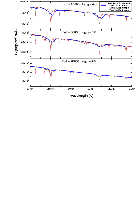
The improvement of non-LTE models over previous models for these stars is significant. Figure 1 shows a comparison between LTE and non-LTE models for solar chemical abundance. From this figure it is clear that for higher temperatures non-LTE models make a significant difference, as already shown by Hauschildt et al. (1999). They argue that LTE models are adequate for solar-type stars, whereas for cooler and hotter stars the non-LTE effects become progressively more important.

Figure 1: Comparison between non-LTE and LTE models for solar abundance. Dashed: Kurucz(LTE) at the original published resolution of 20 Å; dotted: Kurucz (LTE) recomputed with SYNSPEC, at a resolution of 0.3 Å; solid: TLUSTY (non-LTE) and SYSNSPEC, at a resolution of 0.3 Å. The new non-LTE models are a dramatic improvement over previous model spectra for T_eff $\geq$ 27500 K.

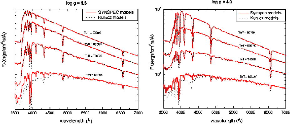
As LTE effects are still negligible for models cooler than T_eff $\leq$ 27000 K, we adopted Kurucz atmosphere models for these temperatures. We chose to use the Castelli, Gratton, & Kurucz (1997) models, which do not include overshooting. The high-resolution spectra were generated using SYNSPEC. We decided to perform the spectrum synthesis with SYNSPEC instead of SYNTHE (Kurucz & Avrett 1981) as the former program is better documented and consequently less prone to user errors (SYNSPEC has a very detailed manual available online, which is not true for SYNTHE). Besides that, SYNSPEC has some physical advantadges, as, for example, flexibility in handling atomic data or more recent hydrogen and helium line broadening tables. We compared these models with previously generated low resolution Kurucz models, which are known to reliably reproduce the continuum fluxes for this temperature range (4750 K $\leq$ T_eff $\leq$ 27000 K). This can be seen in Figure 2, where our high-resolution models were smoothed with a gaussian filter to mimic the Kurucz resolution ($\sim$20 Å). As this figure shows, our models agree quite well with the Kurucz models down to the temperature of 7000 K. As demonstrated by Murphy & Meiksin (2004), the spectra are not expected to be identical, since Kurucz models are flux distributions coming directly from the model atmospheres and not generated by a spectral synthesis.

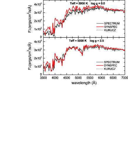
For T_eff $\leq$ 7000 K molecules start to be important in the spectra, and we found the latest publicly available version of SYNSPEC to be inadequate, due to its treatment of the molecular partition functions. This can be clearly seen in Fig. 2. For stars with temperatures between 4750 K and 8250 K, we still used Kurucz model atmospheres, but now we generated the synthetic profile with the code SPECTRUM. This code is optimized for this temperature range and produces reliable results, as shown in Figure 3. The upper limit was chosen based on comparisons between the two models and corresponds to the temperature where the differences between the two are minimal.

Figure 2: Comparison between the SYNSPEC models used in our library and previously published Kurucz models. The SYNSPEC models were smoothed to the resolution of Kurucz models. Left: log g =1.5; right: log g = 4.0. SYNSPEC fails for T_eff $\leq$ 7000 K due to inadequate molecular partition functions. Solar abundance for all models.

For even lower temperatures (T_eff $\leq$ 4500 K) Kurucz model atmospheres themselves fail. These very cool stars are still very hard to reproduce, mainly because molecular features dominate the spectrum. Phoenix models are a better choice for this temperature range because they consider triatomic and larger molecules (676 species in total) and are able to account for spherical geometry. For models with low gravities (log g $\leq$ 3.5), this can be a dominant effect for the correct calculation of the atmospheric structure and the synthetic spectrum (Aufdenberg et al. 1998, 1999). Bertone et al. (2004) compares models from Kurucz’s ATLAS9 and Phoenix/NextGen models. They argue that ATLAS provides in general a sensibly better fit to observed spectra of giants and dwarf stars. Their models, however, are different from the ones used in our library. Bertone et al. used previous-generation Phoenix models, which, for example, assume a mixing length parameter of 1 instead of 2. Two is preferred by hydrodynamic models. Aufdenberg et al. (1998, 1999) compared interferometry data and the Phoenix models for M giants with very low gravities, and found a very good agreement.

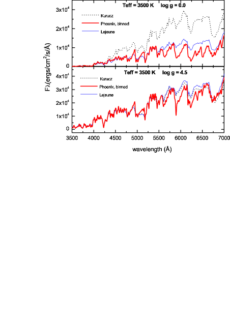
The publicly available models on the webpage have only intermediate resolution (2 Å). Therefore we calculated a new grid with higher resolution. Our grid of high-resolution spectra was created for M = 1 M_☉, a mixing length parameter set to 2.0, spherical geometry, and constant microturbulent velocity of 2 km s^-1. The grid covers T_eff from 3000 K to 4500 K, with a 500 K step, and –0.5 $\leq$ log g $\leq$ 5.5. Dust is allowed to form, but assumed to dissipate immediately after formation. The models are metal line-blanketed. Figure 4 shows a comparison between Kurucz, Lejeune and Phoenix models. The Lejeune models (Lejeune, Cuisinier, & Buser 1997) were constructed applying a correction function to the original Kurucz models, in order to yield synthetic colors matching the empirical color-temperature calibrations derived from observations. This correction is only relevant for low-temperature stars (T_eff $<$ 5000 K) and is more important for low- than for high-gravity stars. We emphasize the excellent agreement of the self-consistent Phoenix models with the empirically adjusted Lejeune models.

Figure 3: Comparison between the Kurucz, SYNSPEC and SPECTRUM models. The SYNSPEC and SPECTRUM models were smoothed to the resolution of Kurucz models. SPECTRUM generates spectra in excellent agreement with the original Kurucz models. Solar abundance for all models.

Figure 4: Comparison between the Phoenix, Kurucz and Lejeune models. The Phoenix models were smoothed to the resolution of Kurucz models. The Phoenix models used in our library agree with the empirically adjusted Lejeune models. Solar abundance for all models.

Models for effective temperatures lower than about 2500 K – 3000 K need to include the effects of dust formation and/or dust opacity. This significantly changes the physics of the model atmospheres and the formation of the spectrum. From the point of view of stellar populations, these stars are not so important because their contribution to the total luminosity is insignificant. Besides, the evolutionary tracks in Starburst99 and sed@ are not precise for this mass range. Therefore we made no further effort to optimize the library spectra in this temperature regime.

In all spectra, the maximum distance between two neighboring frequency points for evaluating the spectrum is 0.01 Å. The spectra were, however, degraded to a final resolution of 0.3 Å, assuming a rotational and instrumentational convolution for each star. A T_eff-dependent rotational velocity was assumed for all spectra. For stars with T_eff $\geq$ 7000 K, we assumed a rotational velocity of 100 km s^-1. For stars with 6000 K $\leq$ T_eff $\leq$ 6500 K, we assumed 50 km s^-1, and for lower temperatures a value of 10 km s^-1 was used. These values are typical for stars in these T_eff ranges (de Jager 1980). All the spectra are sampled in air wavelengths. Phoenix models were originally generated for vacuum wavelengths, but were subsequently transformed to air wavelengths. The final library contains 414, 413, 416 and 411 spectra for 1/10, half, solar and twice solar chemical composition, respectively (see Table 1). The grid coverage is illustrated in Figure 5. Isochrones obtained with the evolutionary tracks from the Padova group (Girardi et al. 2002) have been overplotted. The figure illustrates the homogeneous coverage of this stellar library. The large number of grid points reduces the uncertainties of the nearest neighbor assignation assumed in many synthesis codes. Except for the Wolf-Rayet phase at the highest T_eff and lowest log g, our library covers all evolutionary phases.

Figure 5: Log g vs. T_eff diagram. Points represent the stellar library grid. Lines are isochrones of stellar populations that evolve following the Padova evolutionary tracks with solar chemical abundances.

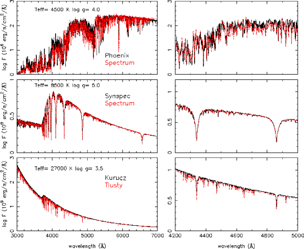
In order to illustrate possible systematic differences in the parts of the library where we switch the codes used to generate the spectra (stellar atmospheres and/or numerical method), in Figure 6 we compare spectra at three effective temperatures (27000 K, 85000 K, and 45000 K), the points where the changes occur. It is clear from this figure that the transitions are smooth, since the models on this transition points are very similar.

Figure 6: Comparison between the spectra obtained with different codes. Botton: Teff= 27000 K obtained with Kurucz+Synspec (full black line) and Tlusty+Synspec (dotted red line) stellar atmosphere models. Middle: Teff= 8500 K obtained with Kurucz+Synspec (full black line) and Kurucz+Spectrum (dotted red line). Top: Teff= 4500 K obtained with Phoenix (full black line) and Kurucz+Spectrum (dotted red line). Solar abundance for all models.

4 Properties of the synthesized spectra

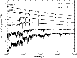
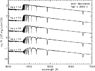
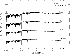
The library is part of the sed@ and Starburst99 codes. The implementation of the library into the codes is discussed in GD04. The general behavior of the models is shown on Figures 7 to 9. Fig.7 shows the variations in the spectra with T_eff for main-sequence stars with solar abundance. Metallic absorption lines and molecular features increase with decreasing temperature. The molecular features dominate the spectra at very low temperatures. Fig.8 shows the response of the spectra to gravity for a star with T_eff = 9000 K and solar abundance. The width (and equivalent width) of the H lines decreases with gravity. Fig.9 illustrates the variation with chemical abundance for a main-sequence star with T_eff = 6000 K. The blanketing effect increases from low to high chemical abundances, and from the red to the blue part of the spectra.

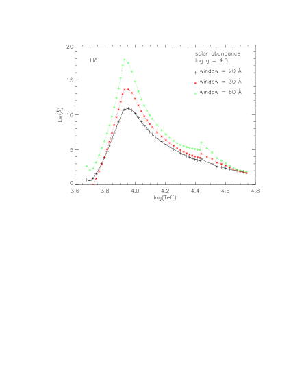
We also calculated the equivalent widths for the most important H and He lines in these synthetic spectra. We tested different spectral windows of 20 Å, 30 Å and 60 Å for the hydrogen lines, in order to measure the contribution of weaker lines adjacent to the spectral index. The comparison between these windows can be seen in Figure 10, where we have plotted the predicted H$\delta$ equivalent widths for the three window sizes. Fig.10 suggests a rather significant influence of the window size due to the inclusion of numerous, weak metallic absorption lines. For the following discussion, all measurements refer to the 30 Å window, which we adopted as the default for all Balmer-line measurements. Table 2 summarizes the window definitions. A small discontinuity at log T_eff = 4.4 (T_eff = 27500 K) is visible in Fig.10. This is the temperature where we switch to the OSTAR2002 grid, meaning that this is where we switch from non-LTE to LTE. Besides that, the models in this grid were calculated with a very detailed and extended line list, accounting for the blanketing effects of millions of Fe and Ni lines. Therefore weak lines appear in these models, falling into the line windows we used and increasing the equivalent widths. This effect is present in Figures 11 – 14 as well.

We measured the H and HeI equivalent widths in two ways: (a) using the theoretical continuum, calculated by each code used, that would give the equivalent widths of the lines in a strict theoretical definition; (b) using a pseudo-continuum, which was determined by fitting a first-order polynomial to the windows defined in Table 2. This simulates the values that we could measure observationally. The equivalent widths for these lines were calculated only for stars with T_eff $\geq$ 5000 K, since at lower temperature the H lines become very weak, and the measurement would be contaminated by the surrounding metallic lines. For example, at T_eff = 4500 K and log g = 4.0, the H$\gamma$ line center is only 5% below the continuum value.

Figure 7: Dependence of representative spectra on T_eff.

Figure 8: Dependence of representative spectra on log g. The spectra were shifted by a constant value for clarity.

Figure 9: Dependence of representative spectra on the chemical composition. The spectra were shifted by a constant value for clarity.

Table 2: Line and continuum windows used for the equivalent width measurements.

	Blue Continuum	Line	Red Continuum
H$\delta$	4012.1 – 4019.9	4087.1 – 4117.1	4157.9 – 4169.0
H$\gamma$	4262.0 – 4270.1	4325.0 – 4355.0	4445.0 – 4453.1
H$\beta$	4769.9 – 4781.9	4847.0 – 4877.0	4942.1 – 4954.1
H$\alpha$	6506.0 – 6514.1	6548.0 – 6578.0	6611.9 – 6620.0
HeI $\lambda$4026	4012.1 – 4019.9	4019.9 – 4031.0	4157.9 – 4169.0
HeI $\lambda$4471	4445.0 – 4453.1	4463.9 – 4478.0	4493.0 – 4503.0
HeI $\lambda$5876	5834.9 – 5845.1	5870.9 – 5879.9	5903.9 – 5912.0

Figure 10: Comparison between the H$\delta$ equivalent width measured with different apertures. The measurements are for log g = 4 and solar abundance. The equivalent width was calculated as the integrated flux under a pseudo-continuum defined after fitting a linear function to the continuum windows defined in Table 2. The 30 Å line window is defined in Table 2. The boundaries for the 20 Å and 60 Å windows are 4092 – 4112 Å and 4070 – 4130 Å, respectively.

The equivalent widths of H$\delta$, H$\gamma$, H$\beta$ and H$\alpha$ as a function of T_eff for main-sequence stars (log g = 4.0) at solar abundance are shown for the theoretical and pseudo-continuum in the left and right panels of Figure 11, respectively. The equivalent widths calculated with either method agree quite well for stars with T_eff $\geq$ 7000 K. For lower temperatures, molecular lines and bands are very strong, and the placement of the pseudo-continuum does not agree with the theoretical continuum anymore. While the pseudo-continuum is affected by absorption, the real continuum is not, which causes an increase in the equivalent widths measured with this method.

Figure 12 shows the dependence of the H$\gamma$ equivalent width on gravity. The equivalent width of this figure was calculated using the pseudo-continuum. H$\gamma$ (and all the other Balmer lines) are rather sensitive to gravity and temperature, making them an efficient tool for the determination of the fundamental stellar parameters.

Figure 11: Equivalent width of the Balmer lines as a function of the effective temperature for log g = 4.0 and solar abundance. The equivalent widths were measured in windows of 30 Å. The left panel shows the equivalent width calculated as the integrated flux under the real continuum. The right panel shows the equivalent width calculated as the integrated flux under a pseudo-continuum defined after fitting a linear function to the continuum windows defined in Table 2.

Figure 12: Equivalent width of H$\gamma$ as a function of the effective temperature. Each curve corresponds to a different value of the gravity. The chemical abundance is solar and the width of the window used to compute the equivalent widths is 30 Å.

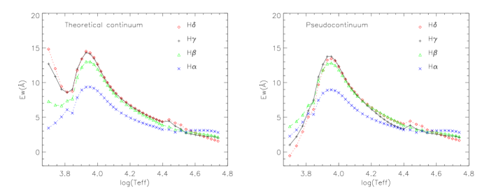
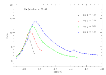
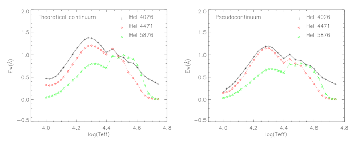
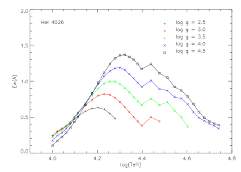
Figure 13 shows the equivalent width of selected HeI lines as a function of T_eff for main-sequence stars. The definition of the continuum is the same as before. The dependence on gravity is in Figure 14. The equivalent width was calculated using the pseudo-continuum. There is an increase of the equivalent width at T_eff $<$ 10000 K which is not due to an increase in HeI absorption, but to the increase of metallic lines that fall into the windows used for the equivalent widths measured. The equivalent width of these lines is insignificant for these temperatures. Therefore we truncated the graphs at T_eff = 10000 K in Fig.13 and 14.

As expected, the equivalent widths of the H and HeI lines are not affected by chemical abundance changes.

Figure 13: Equivalent width of the HeI lines ($\lambda$4026, $\lambda$4471 and $\lambda$5876) as a function of the effective temperature for log g = 4.0 and solar abundance. The left panel shows the equivalent width calculated as the integrated flux under the real continuum. The right panel shows the equivalent width calculated as the integrated flux under a pseudo-continuum defined after fitting a linear function to the continuum windows defined in Table 2.

Figure 14: Equivalent width of HeI $\lambda$4026 as a function of the effective temperature. Each curve corresponds to a different value of the gravity.

One of the most challenging problems in interpreting an observed galaxy spectrum is the difficulty to disentangle age and metallicity effects. Until very recently this analysis has relied metallic indices. Particularly effective is the comparison between lines which are mainly sensitive to the main sequence turnoff temperature, like the Balmer lines, and metallic indices sensitive to the temperature of the giant branch, which depends on metallicity (Worthey 1994; Buzzoni, Mantegazza & Gariboldi 1994). However, it is clear that fitting the whole spectrum instead of calculating indices should be much more efficient. This is a major motivation for generating this library.

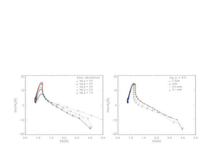
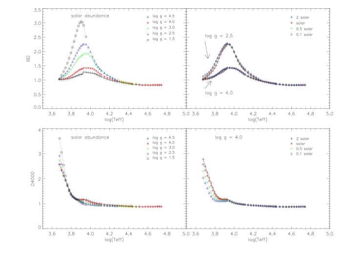
As a consistency check, we calculated several widely used metal indices to test the behavior of our library. The Balmer discontinuity is an important age diagnostic in the optical continuum of a stellar population. While the 4000 Å break is produced by a blend of metallic lines around 3800 – 4000 Å, the Balmer discontinuity depends on the convergence of the Balmer series below 4000 Å. Different definitions can be adopted to measure this discontinuity, depending on the stellar age we are interested to measure. The 4000 Å break defined by Balogh (D4000, Balogh et al. 1999) is suitable to study the general change of the discontinuity for intermediate and old stellar populations while the Balmer discontinuity defined by Rose (BD, Rose, Stetson, & Tripico 1987) is used to date young stellar populations. Balogh et al. use 100 Å continuum bandpasses to measure the break (3850 – 3950 Å and 4000 – 4100 Å). The Balmer discontinuity as defined by Rose is the ratio of the average flux in two narrow bands at 3700 – 3825 Å and 3525 – 3600 Å. Recently, the 4000 Å break has been used in combination with the H$\delta$ absorption line to date stellar populations of galaxies in the Sloan Digital Sky Survey release (Kauffmann et al. 20003a,b,c). The definition of H$\delta_{A}$ of Worthey & Ottaviani (1997) uses a central bandpass (4082 – 4122 Å) bracketed by two pseudo-continuum bandpasses (4030 – 4082 Å and 4122 – 4170 Å). Figure 15 shows D4000 as a function of the equivalent width of H$\delta$ defined by Worthey & Ottaviani (1997) (Ew(H$\delta_{A}$)) for different values of gravity (left panel) and chemical abundance (right panel). Note the strong correlation between these indices for intermediate and low temperature stars (D4000 decreases with temperature) making this plot suitable for studying intermediate and old stellar populations. Figure 16 shows D4000 and BD as a function of T_eff for different values of log g and chemical abundances.

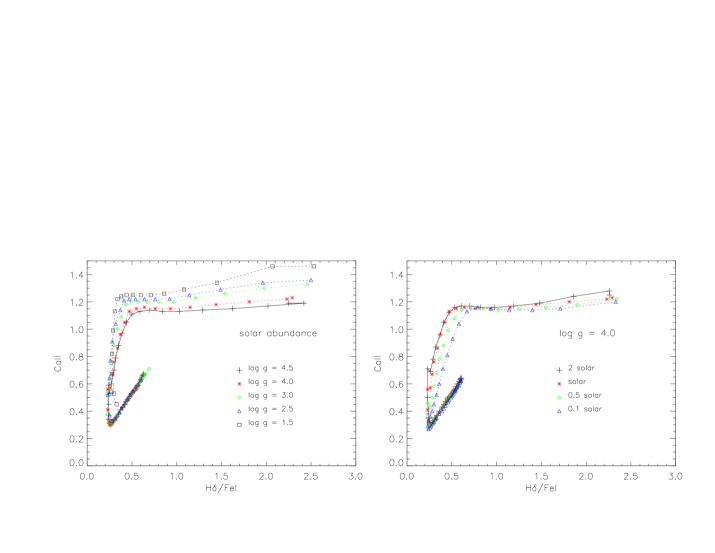
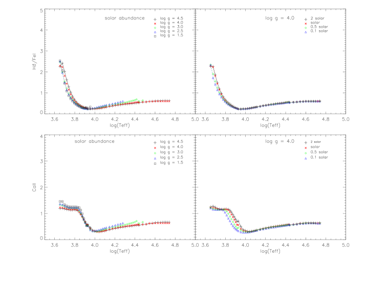
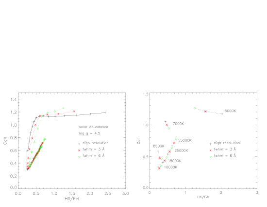
Rose et al. (1987) proposed to use the ratio of the central line depths of two neighboring spectral line features, which has several advantages with respect to an equivalent width index. In particular, it is independent of the placement of the pseudo-continuum, insensitive to reddening and only slightly dependent of the resolution. Figure 17 is a plot of the Rose indices CaII vs. of H$\delta$/FeI for different values of gravity and chemical abundances. Figure 18 shows each of these indices individually as a function of T_eff for different values of gravity (left panels) and chemical abundance (right panels). CaII is the ratio of the residual central intensity of CaII + H$\epsilon$ and CaIIK lines. H$\delta$/FeI is the ratio of the residual central intensity of H$\delta$ to that of the FeI$\lambda$4045 line. Figure 19 shows the comparison between the Rose indices for different spectral resolutions of the original spectra. Our models confirm the small dependence of these indices with resolution, up to a temperature of $\sim$ 7000 K. Below this temperature, the dependence becomes stronger. However, this relation is not useful for such low temperatures since the H lines are very weak.

Figure 15: Behavior of D4000 versus Ew(H$\delta_{A}$) for different gravities (left) and chemical abundances (right).

Figure 16: Behavior of D4000 and BD with T_eff. Top left: BD vs. T_eff for different log g at solar abundance; top right: BD vs. T_eff for different abundances and log g=2.5 and 4.5; bottom left: D4000 vs. T_eff for different log g at solar abundance; bottom right: D4000 vs. T_eff for different abundances and log g=4.0.

Figure 17: Behavior of the Rose indices CaII and H$\delta$/FeI for different gravities (left) and chemical abundances (right).

Figure 18: Behavior of the Rose indices H$\delta$/FeI and CaII with T_eff. Top left: H$\delta$/FeI vs. T_eff for different log g at solar abundance; top right: H$\delta$/FeI vs. T_eff for different abundances and log g=4.0; bottom left: CaII vs. T_eff for different log g at solar abundance; bottom right: CaII vs. T_eff for different abundances and log g=4.0.

Figure 19: Rose indices measured in the original spectra and in the spectra degraded to a resolution of fwhm= 3 Å and 6 Å (left). In the right panel we restricted the data points to a few representative temperatures and connected models with identical temperatures and different resolution to improve clarity.

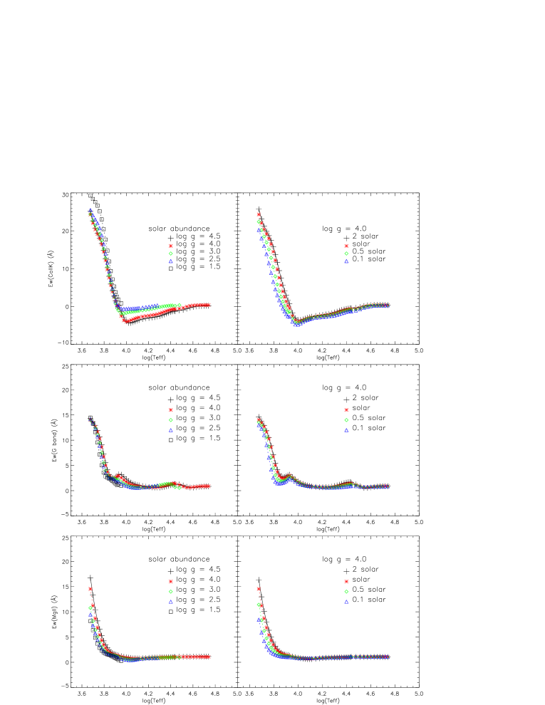
In a series of papers starting in mid 1980’s, Bica & co-workers have explored a stellar populations synthesis technique known as Empirical Population Synthesis, which decomposes a given galaxy spectrum into a combination of observed spectra of star clusters (Bica & Alloin 1986, Bica 1988, and Bica, Alloin, & Schmitt 1994). In practice, instead of modeling the F_λ spectrum directly, this method synthesizes a number of absorption line equivalent widths and continuum colors, which are used as a compact representation of F_λ. The equivalent widths and colors are measured relative to a pseudo-continuum defined at pre-selected pivot wavelengths, which is traced interactively over the observed spectrum (see Cid Fernandes, Storchi-Bergmann, & Schmitt 1998 for an illustrated discussion). We present some indices measured in Bica’s system. Figure 20 shows the dependence of Ew(CaIIK), Ew(G band) and Ew(MgII) on temperature for different values of chemical abundance and gravity. The windows used for each of these indices are 3908 – 3952 Å, 4284 – 4318 Å, and 5156 – 5196 Å, respectively. All of these indices are very useful tools to study intermediate and old stellar populations, since they are very sensitive for low- and intermediate-temperature stars.

Figure 20: Behavior of the Bica indices with temperature.

5 comparison with empirical libraries

The decisive test for the reliability of our synthetic library spectra is a comparison with observed stellar spectra. Recently, two empirical libraries have been made available by Le Borgne et al. (2003) and Valdes et al. (2004) which are suitable for such a test.

Le Borgne et al. (2003) compiled the STELIB library, a collection of 249 stellar spectra at 3 Å resolution covering a wide parameter space in T_eff, log g and [Fe/H]. We selected representative spectra whose stellar parameters are sufficiently close to our grid points for a useful comparison. Since the empirical spectra are affected by interstellar reddening, we corrected them using the A_v values given by Le Borgne et al. The reddening law of Cardelli, Clayton, and Mathis (1989) was used.

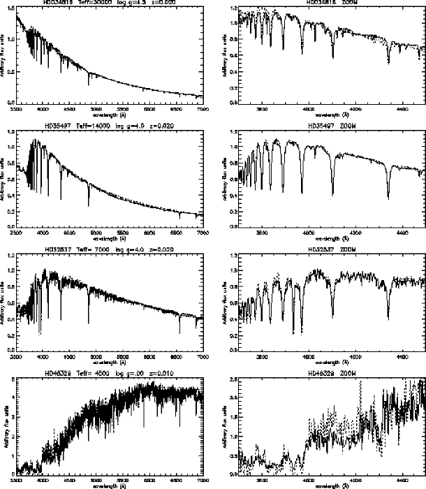
A comparison between our models and selected STELIB stars is in Figure 21. The models were smoothed with a gaussian filter to the STELIB resolution of 3 Å. The spectra were normalized at 4020 Å. The left panels in this figure reproduce the full spectra range, and the right panels show a zoomed view of the region around the 4000 Å break. The stellar parameters given by STELIB for each star are summarized in Table 3. For comparison, the corresponding parameters of the synthetic spectra are given at the top of each panel in Fig. 21. No effort was made to interpolate in our theoretical grid. The best fitting model was selected from a $\chi^{2}$ fit of the synthetic spectra to the observations. Considering that no optimization was performed, the agreement over a broad parameter range is quite satisfactory. We are also reproducing in this figure one of the worst cases: HD 48329, a G8 supergiant. Our half-solar model appears to underestimate the blanketing around 4100 Å. Remember that for this temperature range the “half solar” models have actually one third solar abundances, what may be the reason for that.

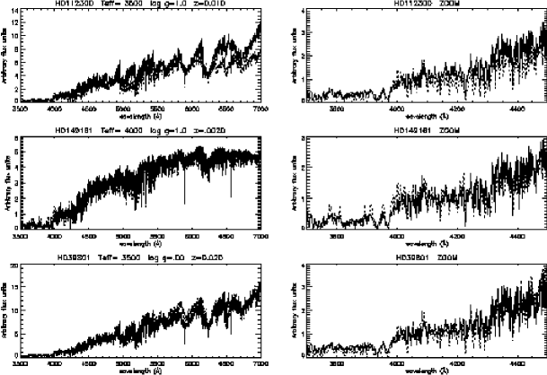
In order to further explore the quality of our synthetic library at very low temperatures, we utilized the Indo-US library of Valdes et al. (2004). This library has particularly complete coverage at the low-temperature end. It includes reddening corrected spectra for 1273 stars with a resolution of $\sim$ 1 Å. We performed a comparison with our models following the same rules as we used for the STELIB library. The selected stars are summarized in Table 4, and the comparison is plotted in Figure 22. The three synthetic spectra in this temperature regime were generated with Phoenix. Given the complexity of the line blanketing, the agreement between models and observations is rather gratifying.

Table 3: Parameters of the STELIB stars used in Figure 21.

Star	Spectral type	Teff	log g	[Fe/H]	Av
HD 034816	B0.5IV	30262 K	4.18	0.05	0.02
HD 35497	B7III	13622 K	3.80	0.41	0.03
HD 32537	F0V	7031 K	4.04	-0.23	0.4
HD 48329	G8Ib	4540 K	0.88	-0.04	0.0

Table 4: Parameters of the Indo-US stars used in figure 21.

Star	Spectral type	Teff	log g	[Fe/H]
HD 112300	M3III	3700 K	1.3	-0.16
HD 149161	K4III	3910 K	1.6	-0.23
HD 39801	M1	3540 K	0.0	0.05

Figure 21: Comparison between representative from the STELIB library (solid line) and synthetic spectra having similar stellar parameters (dotted line). Left panels: full wavelength range; right panels: zoomed view of the region around the 4000 Å break.

Figure 22: Comparison between representative from the Indo-US library (solid line) and synthetic spectra having similar stellar parameters (dotted line). Left panels: full wavelength range; right panels: zoomed view of the region around the 4000 Å break.

6 Summary and conclusions

We generated a grid of stellar atmospheres and synthetic spectra covering the optical range from 3000 Å to 7000 Å, with a sampling of 0.3 Å. The grid spans a range of effective temperatures from 3000 K to 55000 K, and gravities from –0.5 to 5.5 for four different metallicity values (one tenth solar, half solar, solar and twice solar). The spectra were generated using most up-to-date codes available in the literature for each temperature and gravity values. The library contains 1654 spectra, incorporating the last improvements in stellar atmospheres: non-LTE line-blanketed models for hot stars (T_eff $\geq$ 27500 K) and Phoenix LTE line-blanketed models for cool stars (3000 K $\leq$ T_eff $\leq$ 4500 K). We used Kurucz atmosphere models for the parameter space in between, but the codes SPECTRUM and SYNSPEC were used to generate the high-resolution spectral profiles.

We calculated equivalent widths of H and HeI lines to understand the general behavior of our library. We found, as expected, that these lines are very sensitive to gravity and temperature, what makes them an efficient tool for the determination of fundamental stellar parameters. We also calculated some other metallic indices widely used in the analysis of stellar populations. We show a comparison between the 4000 Å break defined by Balogh et al. (1999), D4000, and the Balmer discontinuity defined by Rose et al. (1987), BD. D4000 is suitable for studying the discontinuity for intermediate and old stellar populations, while BD can be used to date young stellar populations. We also show comparisons of D4000 vs. Ew(H$\delta_{A}$), where Ew(H$\delta_{A}$) is the equivalent width of H$\delta$ as defined by Worthey & Ottaviani (1987). There is a strong correlation between these indices for low and intermediate temperature stars, making them useful for studying intermediate and old stellar populations. We show the behavior of the CaII and H$\delta$/FeI indices defined by Rose et al. (1987) and the Ew(CaIIK), Ew(G Band) and Ew(MgII) defined by Bica (Bica & Alloin 1986, Bica 1988) for our library.

A final consistency check was done by comparing our theoretical models with the empirical libraries of Le Borgne et al. (2003) and Valdes et al. (2004). We found that the agreement between models and observations is excellent.

This library constitutes the most comprehensive theoretical stellar library for stellar population synthesis so far, not only because of its optimal parameter space coverage, but also because of its superior resolution and the input physics in the models. The library is available at http://iaa.csic.es/$\sim$rosa and http://www.astro.iag.usp.br/$\sim$lucimara/library.html.

References

- (1) Allard, F., & Hauschildt, P. H. 1995, ApJ, 445, 443
- (2) Allard, F., Hauschildt, P. H., Alexander, D. R., & Schweitzer, A. 2001, ApJ, 556, 337
- (3) Allard, F., & Hauschildt, P. H. 1995, ApJ, 445, 443
- (4) Asplund, M. 2003, in: Elemental Abundances in Old Stars and Damped Lyman- Systems, IAU Joint Discussion, 15, 8
- Aufdenberg, Hauschildt, Shore, & Baron (1998) Aufdenberg, J. P., Hauschildt, P. H., Shore, S. N., & Baron, E. 1998, ApJ, 498, 837
- (6) Aufdenberg, J. P., Hauschildt, P. H., Sankrit, R. & Baron, E. 1999, MNRAS, 302, 599
- (7) Balogh, M. L., Morris, S. L., Yee, H. K. C., Carlberg, R. G., Ellingson, E. 1999, ApJ, 527, 54
- (8) Baraffe, I., Chabrier, G., Allard, F., & Hauschildt, P.H. 1995, ApJ, 446, L35
- (9) ————- 1997, A&A, 327, 1054
- (10) ————- 1998, A&A, 357, 403
- (11) Bertone, E., Buzzoni, A., Chavez, M., & Rodriguez-Merino, L. H. 2004, AJ, 128, 829
- (12) Bica, E. 1988, A&A , 195, 76
- (13) Bica, E., & Alloin, D. 1986, A&A, 166, 83
- (14) Bica, E., Alloin, D., & Schmitt, H. 1994, A&A, 283, 805
- (15) Burstein, D., Faber, S., Gaskell, B. M., & Krumm, N. 1984, ApJ, 287, 586
- (16) Buzzoni, A., Mantegazza, L., & Gariboldi, G. 1994, AJ, 107, 513
- (17) Cananzi, K., Augarde, R. & Lequeux, J. 1993, A&AS, 101, 599
- (18) Cardelli, J. A., Clayton, G. C., & Mathis, J. S. 1989, ApJ, 345, 245
- (19) Castelli, F. 1999, A&A, 346, 564
- (20) Castelli, F., Grotton, R. G. & Kurucz, R. L.,1997, A&A, 318, 841
- (21) Cenarro, A. J., Cardiel, N., Gorgas, J., Peletier, R. F., Vazdekis, A., & Prada, F. 2001, MNRAS, 326, 959
- (22) Cid Fernandes, R., Storchi-Bergmann, T., & Schmitt, H. 1998, MNRAS, 297, 579
- (23) de Jager, C. 1980, The Brightest Stars (Dordrecht: Reidel), 50
- (24) Gardiner, R. B., Kupka, F., & Smalley, B. 1999, A&A, 347, 876
- (25) Girardi, L., Bertelli, G., Bressan, A., Chiosi, C., Groenewegen, M. A. T., Marigo, P., Salasnich, B., & Weiss, A. 2002, A&A, 391, 195
- (26) González Delgado, R. M., & Leitherer, C. 1999, ApJS, 125, 479
- (27) González Delgado, R. M., Heckman, T., & Leitherer, C. 2001, ApJ, 546, 845
- (28) González Delgado, R. M., Cerviño, M., Martins, L. P., Leitherer, C., & Hauschildt, P. H. 2004, submitted to MNRAS
- (29) Gray, R. O., & Corbally, C. J. 1994, AJ, 107, 742
- (30) Hauschildt, P. H., & Baron, E. 1999, J. Comput. Appl. Math. 102, 41
- (31) Hauschildt, P. H., Baron, E., Starrfield, S., & Allard, F. 1996, ApJ, 462, 386
- (32) Hauschildt, P. H., Allard, F., & Baron, E. 1999, ApJ, 512, 377
- (33) Hubeny, I. 1988, Computer Physics Comm. 52, 103
- (34) Hubeny, I., & Lanz, T. 1995, ApJ, 439, 875
- (35) Hubeny, I., Lanz, T., & Jeffery, C. S. 1995, Synspec-A User Guide
- (36) Irwin, A. W. 1998, A&AS, 74, 145
- (37) Jacoby, G., Hunter, D. A., & Christian, C. A. 1984, ApJS, 56, 257
- (38) Kauffmann, G., Heckman, T. M., White, S. D. M., Charlot, S., Tremonti, C., Brinchmann, J., Bruzual, G., Peng, E. W., et al. 2003a, MNRAS, 341, 33
- (39) Kauffmann, G., Heckman, T. M., Tremonti, C., Brinchmann, J., Charlot, S., White, S. D. M., Ridgway, S., Brinkmann, J. et al. 2003b, MNRAS, 346, 1055
- (40) Kauffmann, G., Heckman, T. M., White, S. D. M., Charlot, S., Tremonti, C.,Peng, E. W., Seibert, M. et al. 2003c, MNRAS, 341, 54
- (41) Kurucz, R. L. 1979a, ApJS, 40, 1
- (42) Kurucz, R. L. 1979b, Dudley Observatory Report No. 14 ed. A.G.Davis Phillips, 363
- (43) Kurucz, R. L. 1992, in: IAU Symp. 149, The Stellar Populations of Galaxies, ed. B. Barbuy, and A. Renzini (Dordrecht: Reidel), 225
- (44) Kurucz, R. L. 1993a, Atomic Data for Opacity Calculations, Kurucz CD-ROM No.1
- (45) Kurucz, R. L. 1993b, Stellar Atmosphere Programs and 2 km/s Grid, Kurucz CD-ROM No. 13
- (46) Kurucz, R. L. 1993c, Diatomic Molecular Data for Opacity Calculations, Kurucz CD-ROM No. 15
- (47) Kurucz, R. L., & Avrett, E. H. 1981, SAO Spec. Rep. No. 391, 145
- (48) Kurucz, R. L., & Peytremann, E. 1975, SAO Spec. Rep. No. 362, 1219
- (49) Lanz, T., & Hubeny, I. 2003, ApJS, 146, 417
- (50) Le Borgne, J.-F., Bruzual, G., Pelló, R., Lançon, A., Rocca-Volmerange, B., Sanahuma, B., Schaerer, D., Soubiran, C., & Vílchez-Gómez, R. 2003, A&A, 402, 433
- (51) Leitherer, C., Robert, C., & Heckman, T. M. 1995, ApJS, 99, 173
- (52) Leitherer, C., Schaerer, D., Goldader, T. D., González Delgado, R. M., Robert, C., Kune, D. F., de Mello, D., Devost, D., & Heckman, T. M. 1999, ApJS, 123, 3
- (53) Lejeune, T., Cuisinier, F., & Buser, R. 1997, A&AS, 125, 229
- (54) Maraston, C., & Thomas, D. 2000, ApJ, 541, 126
- (55) Murphy, T., & Meiksin, A. 2004, MNRAS, 351, 1430
- (56) Neale, L., & Tennyson, J. 1995, ApJ, 454, L169
- (57) Neale, L., Miller, S., & Tennyson, J. 1996, ApJ, 464, 516
- (58) Pauldrach, A. W. A., Lennon, M., Hoffmann, T. L., Sellmaier, F., Kudritzki, R.-P., & Puls, J. 1998 in Boulder-Munich II: Properties of Hot Luminous Stars, ed I. P. Howarth, P. (San Francisco: ASP), 258
- (59) Pauldrach, A. W. A, Hoffmann, T. L., & Lennon, M. 2001, A&A, 375, 161
- (60) Rose, J. A., Stetson, P. B, & Tripicco, M. J. 1987, AJ, 94, 1202
- (61) Schweitzer, A., Hauschildt, P. H., Allard, F., & Basri, G. 1996, MNRAS, 283, 821
- (62) Sharp, C. M., & Huebner, W. F. 1990, ApJS, 72, 417
- (63) Sneden, C. 1973, Ph.d. Thesis, University of Texas in Austin.
- (64) Steffen, M. & Ludwig, H-G. 1999, in: Theory and Tests of Convection in Stellar Structure eds. Gimenez A., Guinan, E.F., Montesinos, B. (San Francisco: ASP), 217
- (65) Tinsley, B. M. 1980, Fund. Cos. Phys., 5, 287
- (66) Trager, S. C. 2004, in Origin and Evolution of Elements (Carnegie Observatories Astrophysics Series), 391
- (67) Valdes, F., Gupta, R., Rose, J. A., Singh, H. P., & Bell, D. J. 2004, ApJS, 152, 251
- (68) Valenti, J. A., & Piskunov, N. 1996, A&A, 118, 595
- (69) Walborn, N. R., & Fitzpatrick, E. L. 1990, PASP, 102, 379
- (70) Worthey, G. 1994, ApJS, 95, 107
- (71) Worthey, G., & Ottaviani, P. L. 1997, ApJS, 111, 377
- (72) Worthey, G., Faber, S. M., González, J. J., & Burstein, D. 1994, ApJS, 94, 687