Galaxy Groups at ${\bf 0.3\leq z\leq 0.55}$. II. Evolution to ${\bf z\sim 0}$

Abstract

We compare deep Magellan spectroscopy of 26 groups at $0.3\leq z\leq 0.55$, selected from the Canadian Network for Observational Cosmology 2 field survey, with a large sample of nearby groups from the 2PIGG catalogue (Eke et al., 2004). We find that the fraction of group galaxies with significant [Oii]$\lambda 3727$ emission ($\geq$5Å) increases strongly with redshift, from $\sim 29$% in 2dFGRS to $\sim 58$% in CNOC2, for all galaxies brighter than $\sim\hbox{M}_{*}+1.75$. This trend is parallel to the evolution of field galaxies, where the equivalent fraction of emission line galaxies increases from $\sim 53$% to $\sim 75$%. The fraction of emission-line galaxies in groups is lower than in the field, across the full redshift range, indicating that the history of star formation in groups is influenced by their environment. We show that the evolution required to explain the data is inconsistent with a quiescent model of galaxy evolution; instead, discrete events in which galaxies cease forming stars (truncation events) are required. We constrain the probability of truncation ($\hbox{P}_{\rm trunc}$) and find that a high value is required in a simple evolutionary scenario neglecting galaxy mergers ($\hbox{P}_{\rm trunc}\mathrel{\raise 1.50696pt\hbox{$\scriptstyle>$}\kern-6.00006pt\lower 1.72218pt\hbox{{$\scriptstyle\sim$}}}0.3~{}$Gyr^-1). However, without assuming significant density evolution, $\hbox{P}_{\rm trunc}$ is not required to be larger in groups than in the field, suggesting that the environmental dependence of star formation was embedded at redshifts $z\mathrel{\raise 1.50696pt\hbox{$\scriptstyle>$}\kern-6.00006pt\lower 1.72218pt\hbox{{$\scriptstyle\sim$}}}0.45$.

1 Introduction

Star formation rates derived from high redshift UV surveys and low redshift spectral analysis indicate that the global star formation rate has declined since $z\sim 1.5$ by an uncertain factor of between 4.0 and 40.0 (e.g. Lilly et al., 1996; Madau et al., 1998; Wilson et al., 2002; Panter et al., 2003). This evolution is apparently associated with downsizing (Cowie et al., 1999; Kauffmann et al., 2003; Poggianti et al., 2004), such that the characteristic mass of star forming galaxies decreases with time. The precise cause of this decline, however, is unknown. It may be driven by internal (local) processes, leading to the exhaustion of the gas reservoir, or by interactions with the local environment. This is often referred to as the nature versus nurture dichotomy of galaxy evolution.

The properties of a galaxy population are known to be strongly correlated with their local environment (e.g. Dressler, 1980): galaxies in dense environments typically have bulge–dominated morphologies, low star formation rates and HI gas content, and red colours. Large surveys such as the Sloan Digital Sky Survey (SDSS) have shown that both the galaxy colour distribution (e.g. Blanton et al., 2003; Balogh et al., 2004b) and star formation rate distribution (Lewis et al., 2002a; Martínez et al., 2002; Gómez et al., 2003; Balogh et al., 2004a; Kauffmann et al., 2004) depend on local galaxy density over a wide dynamic range. Similar trends have also been determined at redshifts up to $z\sim 0.5$ (Dressler et al., 1997; Balogh et al., 1999; Kodama et al., 2001; Treu et al., 2003). Recently, De Propris et al. (2004) and Balogh et al. (2004b) have shown that, while the fraction of red galaxies in the nearby Universe increases with local density, the colour distribution and median EW[$\rm H\alpha$] of the blue, star-forming galaxies is nearly independent of environment. A similar trend was observed in the $\rm H\alpha$ equivalent width (EW[$\rm H\alpha$]) distribution (Balogh et al., 2004a). A possible interpretation of these trends is that dense environments transform galaxies from blue to red on a relatively short timescale, $\mathrel{\raise 1.50696pt\hbox{$\scriptstyle<$}\kern-6.00006pt\lower 1.72218pt\hbox{{$\scriptstyle\sim$}}}0.5$ Gyr.

In a $\Lambda$CDM Universe, the growth of large scale structure is a consequence of the hierarchical clustering process. It is therefore possible that this clustering process itself could drive the evolution of global star formation, as more galaxies are drawn into dense environments where their star formation rates are somehow suppressed. The fraction of galaxies located in galaxy clusters is only $\sim 10$% even at the present epoch and, thus, such environments alone can not have a large influence on the global star formation rate. However, perhaps over $50\%$ of galaxies are today found in groups of various sizes (Eke et al., 2004) and thus these environments may play a more significant role. Although some proposed mechanisms for transforming galaxies in dense environments, such as ram pressure stripping (Gunn & Gott, 1972; Quilis et al., 2000) are unlikely to be effective in small groups, many other effects, such as strangulation (Larson et al., 1980; Balogh et al., 2000; Cole et al., 2000; Diaferio et al., 2001), tidal interactions (Byrd & Valtonen, 1990; Gnedin, 2003), or galaxy mergers and interactions (e.g Joseph & Wright, 1985; Moore et al., 1996) may be more widespread. In particular, galaxy interactions are likely to be most common in groups, where the velocity dispersion of the groups is not much larger than that of the constituent galaxies (Barnes, 1985; Zabludoff & Mulchaey, 1998; Hashimoto & Oemler, 2000).

Studies of nearby groups (e.g. Zabludoff & Mulchaey, 1998) show that their galaxy populations vary from cluster-like (mostly early types) to field-like (mostly late-types), suggesting that a nurturing process of galaxy evolution may well be taking place (e.g. Zabludoff & Mulchaey, 2000; Hashimoto & Oemler, 2000; Tran et al., 2001). However, galaxy groups are inevitably much more difficult to detect than clusters, with a relative paucity of members and significantly lower density hot plasma. Therefore, in most cases the group selection criteria is either not well understood, or biased in some way. In particular, one successful method has been to search for the most overdense, compact groups (Hickson, 1982; Severgnini & Saracco, 2001; Coziol et al., 2004); however, such systems may be atypical of the average group environment. Today new opportunities are afforded by large, complete catalogues of nearby groups compiled from redshift surveys such as SDSS and the 2dF Galaxy Redshift Survey (e.g. Eke et al., 2004).

One way to directly observe the influence of galaxy groups is to trace their redshift evolution. In rich clusters, a strong evolution in the fraction of blue galaxies, $\hbox{f}_{\rm blue}$, was detected by Butcher & Oemler (1984) and later by others (e.g. Margoniner et al., 2001; De Propris et al., 2003b), although even this result is still a matter of some debate (e.g. Andreon & Ettori, 1999; Andreon et al., 2004). In Allington-Smith et al. (1993), a sample of groups were photometrically selected in the vicinity of bright radio galaxies at low ($z\leq 0.25$) and intermediate ($0.25\leq z\leq 0.50$) redshift. They tentatively confirm an analogous evolution in the fraction of $\hbox{f}_{\rm blue}$ in larger groups. However, the statistical limitations of photometric data are significant, particularly through field contamination. In addition, the radio selection might bias the choice of groups. It is therefore important to repeat this study using a redshift-space selected sample of spectroscopically confirmed groups. Higher redshift catalogues of groups now exist (Cohen et al., 2000; Carlberg et al., 2001b) from which galaxy properties have been analysed. For example, Carlberg et al. (2001a) studied the properties of group galaxies in the CNOC2 group sample at intermediate redshift. Amongst other things, they discovered a trend in the mean galaxy colors, which on average become redder than the field toward the group centers. In Wilman et al. (2004, hereafter Paper I), we present our deeper and more complete spectroscopy in the region of the intermediate redshift CNOC2 groups (Carlberg et al., 2001b). Our data show that the properties of galaxies in intermediate redshift groups are significantly different from those of coeval field galaxies, in that group galaxies are significantly less likely to have ongoing star formation than their field counterparts, and groups also contain a significant excess of bright galaxies ($M_{b_{\rm J}}$$\leq-21$). These results are discussed in detail in that paper.

In this paper, we contrast the properties of our intermediate redshift group sample (Carlberg et al., 2001b, PaperI) with a large sample of galaxy groups at low redshift, selected from the 2dF Galaxy Redshift Survey (2dFGRS, Eke et al., 2004). This allows us to examine the evolution of galaxies in the group environment with purely spectroscopic data and over a significant range of redshift. In Section 2 we introduce our galaxy and group samples at intermediate redshift (CNOC2 - see also PaperI) and locally (2dFGRS). We then go on to ensure a fair comparison between these two populations and the surrounding field by examining the luminosity functions and EW[OII] distributions. In Section 3, we present our results, in which we assess the environmental and evolutionary dependencies of EW[OII] as well as the dependence on other parameters such as galaxy luminosity. We then discuss the scientific implications in Section 4, and present simple models for the star formation history of these galaxy populations to constrain theories of galaxy evolution. Section 5 presents our final conclusions.

Throughout this paper we assume a $\Lambda$CDM cosmology of $\Omega_{M}=0.3$, $\Omega_{\Lambda}=0.7$ and $H_{0}=75$$\rm kms^{-1}Mpc^{-1}$.

2 Data

2.1 CNOC2: The Intermediate Redshift Sample

A complete description of the data and reduction methods can be found in Paper I. In summary, the intermediate redshift group sample is selected from the CNOC2 redshift survey in the range $0.1\leq z\leq 0.55$ (Carlberg et al., 2001b; Yee et al., 2000). We obtained deeper, more complete multi-object-spectroscopy in the regions of 26 of these groups (in 20 fields) at $0.3\leq z\leq 0.55$ using LDSS2 on the 6.5m Baade telescope at Las Companas Observatory in Chile. The fields were chosen to maximize the number of groups in the Carlberg et al. (2001b) sample along the line of sight, within this redshift range. Redshifts were measured for $74\%$ of galaxies targetted with $R_{c}$$\leq 22$ (with $\sim 60\%$ success rate in the faintest bin $21.5<$$R_{c}$$\leq 22$) and galaxies have been reassigned to groups with a new determination of the group velocity dispersion. The galaxies have each been weighted by a factor $W_{C}$ to account for radial and magnitude-dependent selection functions (see Paper I).

The CNOC2 field galaxy sample is defined to include all galaxies within $240\hbox{${}^{\prime\prime}$}$ of a targetted group centre, lying within the redshift range $0.3\leq z\leq 0.55$ but excluding those galaxies assigned to the targetted group to avoid biasing the field towards the group environment. The final magnitude–limited field sample is therefore representative of the Universe in the $0.3\leq z\leq 0.55$ redshift range.

The CNOC2 group sample contains 240 galaxies within $1h_{75}^{-1}$Mpc of the group centre and the field sample contains 334 galaxies.

2.2 2dFGRS: The Local Sample

The local redshift galaxy sample comes from the large 2dFGRS with over 220 000 galaxy spectra selected in the $b_{\rm J}$-band. The galaxy sample is effectively volume limited (with low incompleteness the sample is representative of the whole population) in the redshift range $0.05\leq z\leq 0.1$ for galaxies with $M_{b_{\rm J}}$$\leq-18.85$. Although there were problems with the atmospheric dispersion corrector prior to August 1999 which affect the instrument throughput (Lewis et al., 2002b), we find our results are unchanged if we exclude data obtained in this period.

The 2dFGRS Percolation-Inferred Galaxy Group catalogue (2PIGG Eke et al., 2004) is also based on a friends-of-friends percolation algorithm. An axial ratio (defined as the line-of-sight length relative to the projected spatial length) of $\sim 11$ is used to link 2dFGRS galaxies together, forming a large catalogue of local groups. Velocity dispersions of the 2PIGG (and CNOC2) groups are calculated with the gapper algorithm. Full details of the 2PIGG group-finding algorithm and description of the catalogue can be found in Eke et al. (2004). We only investigate groups with number of known members $N_{m}\geq 10$ because the contamination of that group catalogue with unphysical systems becomes large in smaller groups. We note that the CNOC2 group detection algorithm (Carlberg et al., 2001b) requires more bright members in close proximity to each other, and therefore likely suffers from less contamination. Even with the $N_{m}\geq 10$ requirement for 2dFGRS groups, we find that the range of group velocity dispersion matches that seen in the CNOC2 group sample. From now on we will refer to the 2dFGRS sample simply as the 2dF sample.

The 2dF field is defined as all galaxies in the 2dF galaxy catalogue and represents the global galaxy population in the $0.05\leq z\leq 0.1$ redshift range, within magnitude limits. Since these groups were untargetted, this definition is compatible with our CNOC2 field definition.

The 2dF group sample contains 5490 galaxies within $1h_{75}^{-1}$Mpc of the group centre and the field sample contains 50981 galaxies.

2.3 The galaxy luminosity function in groups and the field

2.3.1 K-corrected rest frame magnitudes

Galaxies in both catalogues are k-corrected to give rest-frame absolute magnitudes in the $b_{\rm J}$-band. The 2dF k-corrections are taken from Norberg et al. (2002), and are generally small. For the CNOC2 survey, k-corrections have been calculated using no-evolution models; we will explore the sensitivity of our results to the assumed model of galaxy evolution in the discussion (Section 4). We note that k+e corrections are also available for galaxies in the original CNOC2 sample (Shepherd et al., 2001). For each galaxy, we first choose a mixture of observed local SEDs (King & Ellis, 1985) for which the model B-I colour matches the observed colour at the given redshift. Then the rest-frame absolute $b_{\rm J}$ magnitude can be determined from the models, given the observed $R_{c}$ magnitude, SED mixture and redshift. The transformation from observed $R_{c}$-band magnitude to rest-frame $b_{\rm J}$ is chosen because it is closely matched at CNOC2 redshifts and because it directly transforms the CNOC2 spectroscopic selection band to the 2dF selection band. Luminosities are then corrected for galactic extinction on a patch-to-patch basis, computed by extrapolating from B and V band extinction values obtained from NED (Schlegel et al., 1998, variation within each patch is negligible). We make no correction for internal extinction, also to allow direct comparison with local galaxies in 2dF.

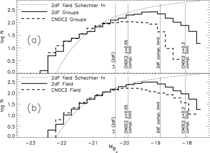
Figure 1: Luminosity functions of the group galaxies (a) and field galaxies (b) for 2dF and CNOC2. Field and Group CNOC2 data are each normalised to match the total number in the CNOC2 sample for $M_{b_{\rm J}}$$<-20.25$

2.3.2 Luminosity limits

Figure 1 shows the superimposed luminosity functions of the 2dF and CNOC2 group and field samples. The volume–limited 2dF sample is $>90\%$ complete for $M_{b_{\rm J}}$$\leq-19$ and so we apply no completeness correction. The Schechter function computed for the 2dF survey (Norberg et al., 2002) is shown for comparison. The CNOC2 galaxies are weighted by $W_{C}$ to correct for the selection function. For comparison between 2dF and CNOC2 group and field samples, the data are normalised so that there is the same number of weighted galaxies brighter than $M_{b_{\rm J}}$$=-20.25$. At these magnitudes, neither sample suffers any incompleteness due to falling below the apparent magnitude limit in the redshift range considered. We note that the enhanced bright to faint galaxy ratio seen in CNOC2 groups relative to the field (Paper I) is also seen in the local 2dF groups.

Also shown in Figure 1 are some critical values of luminosity. The value of $\hbox{M}_{*}$ in Norberg et al. (2002), appropriate to our cosmological model, is $\sim-20.28$, and the 2dF data are complete down to $-18.85$, or equivalently $\sim\hbox{M}_{*}+1.5$. Our CNOC2 data span a wide range in redshift and thus the luminosity limit corresponding to our apparent magnitude limit of $R_{c}$=22 is redshift dependent. At the upper limit of our redshift range, $z=0.55$, a $R_{c}$$=22$ galaxy with a mean k-correction will transform to a rest-frame luminosity $M_{b_{\rm J}}$$=-19.75$ and at the lower redshift limit of $z=0.3$, the same galaxy would transform to $M_{b_{\rm J}}$$=-17.93$. In the case of the reddest galaxies with larger K-corrections, these limits would lie at $M_{b_{\rm J}}$$=-20.07$ ($z=0.55$) and $M_{b_{\rm J}}$$=-18.06$ ($z=0.3$), so we are incomplete below these magnitudes.

Most galaxies in our CNOC2 and 2dF catalogues lie below the brightest CNOC2 luminosity limit of $M_{b_{\rm J}}$$=-20.07$. To enable us to compare the 2dF and CNOC2 galaxy samples independently of differences in the luminosity function (which may be partly intrinsic but is mostly due to selection effects), we choose to apply an additional luminosity weighting to the CNOC2 galaxies. This weighting is calculated within each bin in luminosity using the formula:

$$W_{lum}=N_{2dF}/\sum_{i=1}^{N_{CNOC2}}W_{C}$$ (1)

which corresponds to the difference between the field luminosity functions. It is applied in the range $-20.25\leq$$M_{b_{\rm J}}$$\leq-18.5$, where the CNOC2 data become incomplete at the high redshift end. The choice of a faint final luminosity limit of $M_{b_{\rm J}}$$=-18.5$ ($\sim\hbox{M}_{*}+1.75$) makes maximal use of the data and allows the properties of faint galaxies to be compared with those of brighter galaxies. We emphasize that whilst we are incomplete at $M_{b_{\rm J}}$$\mathrel{\raise 1.50696pt\hbox{$\scriptstyle>$}\kern-6.00006pt\lower 1.72218pt\hbox{{$\scriptstyle\sim$}}}-19.75$ at $z=0.55$ in CNOC2 and $M_{b_{\rm J}}$$\mathrel{\raise 1.50696pt\hbox{$\scriptstyle>$}\kern-6.00006pt\lower 1.72218pt\hbox{{$\scriptstyle\sim$}}}-18.85$ in 2dFGRS, this has no impact on any analysis of galaxy properties as a function of luminosity or on comparisons between the group and field galaxy populations. Also, when studying galaxy properties as a function of luminosity, the analysis is independent of the CNOC2 galaxy weighting, including little effect from weighting by the selection function.

2.4 Measurement of star formation using EW[OII]

The $\rm H\alpha$ emission line disappears entirely from the LDSS2 spectrograph window at $z>0.21$, limited by the instrument sensitivity of the current optics and detector. Therefore,we use the [OII]$\lambda 3727$ emission line equivalent width (EW[OII]) to study the relative levels of star formation in our galaxy samples. In Paper I we outlined the reasons why EW[OII] is sufficient to reveal trends of star formation with galaxy environment. In contrast to using the line flux, the effect of normalising by the continuum when computing the equivalent width reduces uncertainties related to absorption by dust and aperture bias, which are relevant when comparing galaxy properties at different redshifts. In particular, we show in Section 2.4.3 that our analysis is insensitive to aperture bias in EW[OII].

2.4.1 Fair comparison of EW[OII] in 2dF and CNOC2

Details of the CNOC2 equivalent width measurement process are given in Paper I. In 2dFGRS, the equivalent widths of [OII] are measured in a similar way to $\rm H\alpha$ using a completely automated fitting procedure, (see Lewis et al., 2002a, for details). In the fitting of the [OII] emission line, many 2dF measurements are classified as no line present. In our analysis, these are set to 0Å and then all 2dF measurements are smoothed with a gaussian kernel of width 2Å to match the mean error on CNOC2 EW[OII] measurements (much greater than the 2dF line measurement error of $\ll 1$Å). We note that the fraction of galaxies with EW[OII]$>$5Å is unchanged by this smoothing to within $<1\%$. Figure 2 shows the distribution of EW[OII] in our 2dF and CNOC2 group and field galaxy catalogues. We limit the group data to within $1h_{75}^{-1}$Mpc (projected) of the group centre in all cases. The CNOC2 galaxies are weighted by a combined completeness and luminosity weighting to match the 2dF luminosity function, $W_{tot}=W_{C}\times W_{lum}$. The CNOC2 galaxies are limited to $R_{c}$$\leq 22$ and all galaxies are limited to $M_{b_{\rm J}}$$\leq-18.5$. Finally, the distribution of 2dF EW[OII] is normalised to provide an equal number of galaxies to that found in CNOC2, for presentation only. This is done independently for the group and field populations.

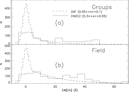
Figure 2: Normalised distributions of EW[OII] of the group (a) and field (b) galaxies in 2dF ($0.05\leq z\leq 0.1$) and CNOC2 ($0.3\leq z\leq 0.55$) samples where $M_{b_{\rm J}}$$\leq-18.5$. The data is normalised to match the total number of galaxies in the CNOC2 analaysis.

2.4.2 Diagnostics of Star Formation for a Galaxy Population

We are motivated by the findings of Strateva et al. (2001); Blanton et al. (2003); Baldry et al. (2004) and Balogh et al. (2004a) who show that galaxy populations have a bimodal distribution in colour and EW[$\rm H\alpha$]. Balogh et al. (2004a, b) show that the fraction of red, passive galaxies is strongly dependent upon local galaxy density. The division between passive and star forming galaxies in the EW[$\rm H\alpha$] distribution occurs at $\sim 4$Å (Balogh et al., 2004a). We do not expect to see such a clear bimodality in EW[OII] since EW[$\rm H\alpha$] $=4$Å typically corresponds to EW[OII] $<2$Å, below the measurement error in EW[OII] for CNOC2. Greater intrinsic scatter in the SFR-[OII] relation than in the SFR-$\rm H\alpha$ relation also works to mask the division between the two populations. Thus, although we cannot cleanly separate the two populations, we impose an arbitrary division at 5Å in the CNOC2 and smoothed 2dF data. We expect the population with EW[OII]$<$5Å to be dominated by the passive population and the population with EW[OII]$\geq$5Å to be dominated by the star-forming population, and this division is sufficient to reveal trends in the data (see e.g. Hammer et al., 1997; Zabludoff & Mulchaey, 2000).

To assess the relative normalisation of the two populations, we define $\hbox{f}_{\rm p}$ as the fraction of passive galaxies. The level of [OII] emission in the star forming galaxies is characterised by $\scriptstyle<$EW[OII]$\scriptstyle|$SF$\scriptstyle>$, which represents the median EW[OII] restricted to star–forming galaxies.

We note that it will also be interesting to derive the fraction of blue galaxies using CNOC2 colours, for a more direct comparison with classical studies of the Butcher-Oemler effect. However, this analysis is not straightforward, because of the complex dependence of CNOC2 colour apertures on galaxy size, galaxy type and redshift; the meagerness of the group red sequence and the difficulties in making a direct comparison with 2dFGRS. Many of these problems can be overcome by computing the fraction of galaxies in each peak of a bimodal colour distribution. This analysis will be presented in a future paper, currently in preparation.

2.4.3 Aperture bias

Systematic effects on the measurements of EW[OII] can be induced by the relative aperture sizes used in the 2dFGRS and CNOC2 spectroscopy. In particular, the 2dF fibres generally sample light from a smaller physical radius than the CNOC2 slits, and this might lead to an overestimate of $\hbox{f}_{\rm p}$ by excluding the star forming regions in face-on disk galaxies. In Appendix A, we use SDSS resolved photometry to estimate the effects of aperture bias across our magnitude range. We find that the fraction of galaxies found in the red peak of the bimodal colour distribution is no greater when considering colours measured inside $3\hbox{${}^{\prime\prime}$}$ SDSS fibres, rather than the total colour. This is because both red and blue galaxies have similar colour gradients, likely due to metallicity rather than star formation. Thus we conclude that the effects of aperture bias do not strongly affect our measurements of $\hbox{f}_{\rm p}$.

3 Results

3.1 Evolutionary and Environmental Dependencies of EW[OII]

A comparison of the 2dF and CNOC2 EW[OII] distributions in Figure 2 shows that the fraction of galaxies in the 0Å peak depends on both epoch and environment. In particular, the 0Å peak in the 2dF data is much more prominent than in the CNOC2 survey, for both field and groups. At both epochs, however, the group galaxy population is more biased towards the 0Å peak than the corresponding field population. We now explore these trends in more detail.

3.1.1 The dependence of $\hbox{f}_{\rm p}$ on redshift, environment and luminosity

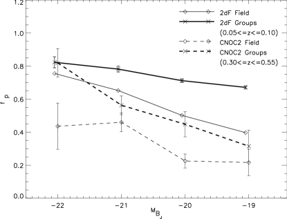
Figure 3: The fraction of galaxies with EW[OII]$<$5Å (the passive population), $\hbox{f}_{\rm p}$, in 2dF and CNOC2 groups (within 1 projected Mpc of group centre) and field, as a function of $M_{b_{\rm J}}$. The 2dF points are slightly offset in $M_{b_{\rm J}}$for clarity.

In Figure 3, the fraction of passive galaxies, $\hbox{f}_{\rm p}$ is plotted against rest-frame $M_{b_{\rm J}}$luminosity. Statistical errors are estimated using a Jackknife resampling method (Efron, 1982). We can see that:

• In all samples, $\hbox{f}_{\rm p}$ is a strong function of luminosity with fainter galaxies far more likely to be star forming than brighter galaxies at equivalent redshifts. This is consistent with many previous results, e.g. Kauffmann et al. (2003).

• $\hbox{f}_{\rm p}$ is significantly greater in the galaxy groups than in the field at both low and intermediate redshift and also right across the luminosity range investigated.

• $\hbox{f}_{\rm p}$ is strongly redshift dependent, both in the field and in galaxy groups. At brighter magnitudes than $M_{b_{\rm J}}$$=-18.5$ ($\sim\hbox{M}_{*}+1.75$ in 2dF), $\hbox{f}_{\rm p}$ in groups evolves from $\sim 42\%$ at $0.3\leq z\leq 0.55$ in CNOC2 to $\sim 71\%$ at $0.05\leq z\leq 0.1$ in 2dF. In our field samples (defined to represent the global population), $\hbox{f}_{\rm p}$ evolves from $\sim 25$% to $\sim 47$% over the same redshift interval. The observed field evolution is consistent with the equivalent strong evolution in the fraction of passive galaxies in the Canada-France Redshift Survey (Hammer et al., 1997) and the global decline in star formation rate since $z\sim 1$ (e.g. Madau et al., 1998). We refer to Whitaker et al., 2004, in preparation, for a more detailed and thorough discussion of the evolution of star formation rate in the global CNOC2 population. This provides a clear analogy at lower densities to the observed evolution of the blue galaxy fraction in clusters (Butcher & Oemler, 1984) and to similar evolution in rich groups, estimated by Allington-Smith et al. (1993) using photometric data.

3.1.2 The properties of the star forming population

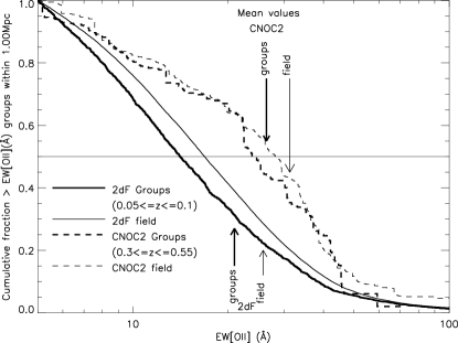
Figure 4: Cumulative distributions of EW[OII] in star forming galaxies in the field and group galaxies of 2dF ($0.05\leq z\leq 0.1$) and CNOC2 ($0.3\leq z\leq 0.55$) samples. The arrows indicate the mean values of EW[OII] for star forming galaxies in each sample.

Figure 5: The median EW[OII] (Å) of star-forming galaxies, $\scriptstyle<$EW[OII]$\scriptstyle|$SF$\scriptstyle>$, in the 2dF and CNOC2 galaxies in the groups (within 1 projected Mpc of group centre) and field, as a function of $M_{b_{\rm J}}$. The 2dF points are slightly offset in $M_{b_{\rm J}}$for clarity.

Figure  4 shows the cumulative distribution of EW[OII], for star forming galaxies only, in the 2dF and CNOC2 group and field samples. Interestingly, the shape of the distribution at a particular epoch (i.e. 2dF or CNOC2) is approximately independent of environment, consistent with earlier analysis of the EW[$\rm H\alpha$] distribution (Balogh et al., 2004a). In the CNOC2 sample, the distribution shows a small enhancement in highly star forming galaxies (EW[OII] $\mathrel{\raise 1.50696pt\hbox{$\scriptstyle>$}\kern-6.00006pt\lower 1.72218pt\hbox{{$\scriptstyle\sim$}}}$ 30Å) relative to the 2dF galaxies in both groups and the field. The mean values of EW[OII] for each sample are indicated by the arrows in Figure 4. These values of 26.4Å (groups) and 31.3Å (field) in CNOC2 are within $\sim 20$ per cent of the mean values in the 2dF (20.9Å in groups and 25.8Å in the field) in 2dF. This difference is much smaller than the evolution in $\hbox{f}_{\rm p}$, which is almost a factor of two. Therefore, the evolution of the total star formation rate is driven more by the evolution of $\hbox{f}_{\rm p}$ than by evolution of the mean properties of star forming galaxies.

In Figure 5 we show the median EW[OII] among star–forming galaxies, $\scriptstyle<$EW[OII]$\scriptstyle|$SF$\scriptstyle>$, as a function of luminosity in the CNOC2 and 2dF group and field samples. Errors are again computed using a Jackknife resampling method. The median EW[OII] is significantly larger for fainter galaxies than for bright galaxies. Furthermore, the evolution in the EW[OII] distribution is largely manifested as an increase in $\scriptstyle<$EW[OII]$\scriptstyle|$SF$\scriptstyle>$ in galaxies with $M_{b_{\rm J}}$$\mathrel{\raise 1.50696pt\hbox{$\scriptstyle>$}\kern-6.00006pt\lower 1.72218pt\hbox{{$\scriptstyle\sim$}}}-21.5$.

3.1.3 Dependence of $\hbox{f}_{\rm p}$ in groups upon group-centric radius and velocity dispersion

Figure 6: The fraction of galaxies with EW[OII]$<$5Å (the passive population) ($\hbox{f}_{\rm p}$) in 2dF and CNOC2 groups, as a function of physical radius. The field level is overplotted and only galaxies where $M_{b_{\rm J}}$$\leq-18.5$ are considered.

In Figure 6 we plot $\hbox{f}_{\rm p}$ as a function of the projected physical distance, dr, from the group centre. It is clear that even in the better sampled 2dF groups, the total fraction of passive galaxies, $\hbox{f}_{\rm p}$ merely declines from $\sim 0.76$ in the innermost $0.125~{}h_{75}^{-1}$ Mpc bin to $\sim 0.65$ in the $0.5~{}h_{75}^{-1}$ Mpc$<\delta(r)\leq 1~{}h_{75}^{-1}$ Mpc bin. This is a weak, but statistically significant trend. The value of $\hbox{f}_{\rm p}$ for the total 2dF field population is $\sim 0.47$, much lower than in the groups. Similarly, in the CNOC2 field, $\hbox{f}_{\rm p}=0.25$ is much smaller than that in the combined group population where $\hbox{f}_{\rm p}=0.42$. We only see a trend with dr in the inner regions of the CNOC2 group population, as shown in Paper I. However, a trend as weak as that seen in 2dF group galaxies would be masked by the statistical errors.

Figure 7: Fraction of galaxies with EW[OII]$<$5Å (passive galaxies) ($\hbox{f}_{\rm p}$) in 2dF and CNOC2 groups, as a function of group line of sight velocity dispersion. The points represent 2dF groups and the triangles represent CNOC2 groups.

We have also investigated how the star formation properties of galaxy groups depend upon the group velocity dispersion, $\sigma(v)_{intr}$. In Paper I we found that there is little dependence of $\hbox{f}_{\rm p}$ on $\sigma(v)_{intr}$ when computed over a wide range of galaxy luminosity. Figure 7 shows $\hbox{f}_{\rm p}$ in CNOC2 and 2dF groups as a function of $\sigma(v)_{intr}$. There are no clear trends visible in Figure 7 other than the evolution from lower $\hbox{f}_{\rm p}$ in CNOC2 groups to that seen in 2dF groups. It is also noticeable that there are very few 2dF groups with high velocity dispersion ($>400$km s^-1) and low $\hbox{f}_{\rm p}$ ($<0.4$), which is a common regime for CNOC2 groups. We note that the enhancement of $\hbox{f}_{\rm p}$ in CNOC2 groups over the CNOC2 field holds when we exclude the 2 groups with velocity dispersion $>600$km s^-1 (for more details see Paper I). The only CNOC2 group with $\hbox{f}_{\rm p}>0.7$ (group 138) is characterized by a high number of confirmed members (35 compared to 19 in the group with the next highest $\sigma(v)_{intr}$) and might better be considered a poor cluster (see e.g. Nakata et al., 2004, for the behaviour of $\hbox{f}_{\rm p}$ in clusters).

4 Discussion

4.1 Implications

We have detected a strong evolution in the fraction of passive galaxies, $\hbox{f}_{\rm p}$ (defined as the fraction of galaxies with EW[OII]$<$ 5Å), in both groups and the field since the Universe was $\sim 1/3$ its current age. Thus, the Butcher–Oemler effect (e.g. Butcher & Oemler, 1984; Margoniner et al., 2001; De Propris et al., 2003b) is not strictly a cluster phenomenon, but is seen both in the general field and in small groups, as previously found by Allington-Smith et al. (1993). These results represent clear evidence that a significant proportion of galaxies in both environments have ceased forming stars since $z\sim 0.5$. A simple argument, neglecting density and luminosity evolution, sees 50% of star forming group galaxies and 35% of star forming field galaxies at $z\sim 0.4$ (CNOC2) becoming passive galaxies by $z\sim 0.1$ (2dF). This evolution is modelled in more detail in Section 4.2.

In contrast, while we find significant redshift evolution in the shape of the EW[OII] distribution for star-forming galaxies, there is little or no dependence on environment. This suggests that this evolution results from very local (i.e. internal to the galaxy) processes that drive an evolution in SFR or metallicity, rather than external, environmental influences. We caution however that amongst star-forming galaxies, it is not possible with current data to rule out an aperture bias in the measurement of EW[OII], which might lead to underestimation of EW[OII] in 2dFGRS star forming galaxies.

In the following sections, we make a first attempt to quantitatively decouple the environmental dependence of galaxy evolution from the global SFR evolution. To fully understand this, we require a homogeneous sample over a large range of environments. We are currently working on providing a fair comparison study in cluster cores (Nakata et al., 2004) using spectroscopic data over an equivalent redshift range. Understanding the importance of galaxy evolution in groups with respect to cluster cores will help to isolate the environments in which galaxy evolution is most active. Complementary studies of the evolution in isolated galaxies would be of especially great benefit to understand the role of environment in driving galaxy evolution, and in particular, the evolution of $\hbox{f}_{\rm p}$.

4.2 Modelling and Interpretation

In this Section, we show how the strong evolution in $\hbox{f}_{\rm p}$ seen in our results can be interpreted in the context of galaxy evolution models. By combining the Bruzual & Charlot (2003) models of luminosity evolution with a range of star formation histories, we attempt to recreate a realistic evolution scenario which can reproduce the observed evolution.

We assume that CNOC2 galaxies represent a population equivalent to the progenitors of the 2dF population; therefore, using the stellar population models of Bruzual & Charlot (2003) it is possible to create mock-2dF populations by evolving the CNOC2 galaxies to the mean redshift of 2dF galaxies ($z_{2dF}$ = 0.08) in accordance with a chosen set of model parameters. We present two model methods with different evolutionary scenarios but similar basic methodology. Both models allow us to estimate the evolution of EW[OII] and $M_{b_{\rm J}}$within a given set of parameters. The quiescent evolution scenario is characterized by the lack of environmental evolution. There are no sudden events which drastically alter a galaxy’s star formation. Bright star-forming galaxies simply decline exponentially in their star formation with a constant e-folding timescale and thus fade in luminosity. In the truncation scenario, we incorporate into our evolution model a probability of each galaxy undergoing a truncation event, in which it suddenly ceases star formation. In this model, there is also a probability that a high redshift field galaxy can infall onto a galaxy group to become a local group galaxy.

4.2.1 The Quiescent Evolution Scenario

Quiescent evolution describes the evolution of galaxies in which every galaxy’s star formation declines over its lifetime with a single e-folding timescale. The modelling procedure for quiescent evolution is described in Appendix B.1, which also describes the effects of allowing each parameter to vary. To investigate the effects of quiescent evolution on $\hbox{f}_{\rm p}$, we choose a control model and an extreme model. For our control model we choose a Kennicutt IMF, a galaxy formation redshift $z_{\rm form}$= 10 and solar metallicity. We also incorporate a two-component dust prescription into the model (Granato et al., 2000). Figure 8 shows $\hbox{f}_{\rm p}$ as a function of luminosity in the observed CNOC2 and 2dF samples, together with the equivalent trend in the evolved CNOC2 population obtained using this model. The evolution of $\hbox{f}_{\rm p}$ in the model significantly underestimates the trend seen in the real data. This is partly because galaxies which become passive also tend to fade into a fainter bin of luminosity, leaving the trend of $f_{p}$ with luminosity approximately unchanged. For our extreme model, we deliberately choose parameters which maximize the evolution in $\hbox{f}_{\rm p}$, as discussed in Appendix B.1. We choose a Salpeter IMF, $z_{\rm form}$= 3, solar metallicity and we ignore the effects of dust. Figure 9 shows the same 2dF and CNOC2 data as in Figure 8 but this time overplotted with the evolved CNOC2 population obtained using this extreme model. In this case, galaxies fainter than $\sim\hbox{M}_{*}-0.5$ still show a significant deficit of passive galaxies (low $\hbox{f}_{\rm p}$) in the evolved CNOC2 galaxies when compared to the data. This provides strong evidence that transformations are required to reproduce the observed evolution in $\hbox{f}_{\rm p}$ both in groups and the global (field) population.

Figure 8: The fraction of passive galaxies, $\hbox{f}_{\rm p}$, in the 2dF (solid line) and CNOC2 group (within 1 projected $h_{75}^{-1}$Mpc of group centre) and field galaxy populations, as a function of $M_{b_{\rm J}}$. The CNOC2 galaxies are shown as observed (dotted-line), and evolved to $z_{2dF}$ using a quiescent model with a Kennicutt IMF, $z_{\rm form}$= 10, solar metallicity and dust extinction (dashed-line). The 2dF points are slightly negatively offset, and the CNOC2 data points slightly positively offset in $M_{b_{\rm J}}$for clarity.

Figure 9: Similar to Figure 8, but assuming an extreme quiescent evolution model for the CNOC2 population, with a Salpeter IMF, $z_{\rm form}$= 3, solar metallicity and no dust extinction (dashed-line). This represents the maximum evolution expected from any realistic quiescent model. The 2dF points are slightly negatively offset, and the CNOC2 data points slightly positively offset in $M_{b_{\rm J}}$for clarity.

4.2.2 The Truncation Scenario

Next we consider a model in which galaxies undergo transformations that cause them to cease forming stars. We have shown in Section 4.2.1 that some form of galaxy transformation appears to be required to reproduce our observed evolution in $\hbox{f}_{\rm p}$. Here, we constrain the probability of these transformations required to match the observed evolution in $\hbox{f}_{\rm p}$ and its dependence upon galaxy luminosity and environment. The modelling procedure is described in Appendix B.2. In this scenario, a CNOC2 galaxy either continues with its e-folding decline in star formation, or has its star formation truncated instantaneously with a probability $\hbox{P}_{\rm trunc}$ per Gyr, at a random point during its evolution to $z_{2dF}=0.08$. The timescale of the transformation is likely to have little effect on the evolution of $\hbox{f}_{\rm p}$. We neglect the possibility that some transformations are accompanied with a strong starburst or involve the merging of galaxies as either of these possibilities cannot be constrained by simply considering the evolution in $\hbox{f}_{\rm p}$. In a later paper we will consider our data in the context of a more complete galaxy formation model (e.g. Cole et al., 2000).

We adopt a realistic set of parameters governing the spectrophotometric evolution, with a Kennicutt IMF, $z_{\rm form}$= 10, solar metallicity and a basic dust prescription (Granato et al., 2000). The progenitors of 2dF group galaxies are chosen by selecting all CNOC2 group galaxies plus a fraction of the CNOC2 field galaxies such that the combined set is made up of $\hbox{$\xi$}_{\rm gr}$% CNOC2 group members and $(1-\hbox{$\xi$}_{\rm gr})$% CNOC2 field galaxies. As our field represents the global population, the progenitors of 2dF field galaxies are simply the CNOC2 field galaxies. Following the model prescription, we obtain best fit values for $\hbox{P}_{\rm trunc}$ as a function of local luminosity and environment to fit the observed evolution in $\hbox{f}_{\rm p}$. Figures  10 and  11 show $\hbox{P}_{\rm trunc}$ as a function of luminosity in groups and the field with $\hbox{$\xi$}_{\rm gr}=100$% (local group members were all group members at $z_{CNOC2}$) and $\hbox{$\xi$}_{\rm gr}=50$% (local group members were $50$% group members and $50$% field galaxies at $z_{CNOC2}$) respectively. We note that adopting a Salpeter IMF does not significantly alter these results.

Figure 10: The probability (per Gyr) that star formation has been truncated ($\hbox{P}_{\rm trunc}$) as a function of $M_{b_{\rm J}}$  as determined by modelling the evolution of $\hbox{f}_{\rm p}$ between the CNOC2 ($0.3\leq z_{CNOC2}\leq 0.55$) and 2dF ($0.05\leq z_{2dF}\leq 0.1$) samples. The crosses represent the group galaxies and the diamonds represent the field population which has been artificially offset by 0.05mag for clarity. Here, there is assumed to be no density evolution, i.e. all group galaxies were already in groups by $z_{CNOC2}$ ($\hbox{$\xi$}_{\rm gr}=100$%). The vertical line represents the location of a $\hbox{M}_{*}$ galaxy in 2dF as determined from the luminosity function of Norberg et al. (2002).

Figure 11: As Figure  10, but assuming local 2dF groups comprise $50$% CNOC2 group galaxies and $50$% CNOC2 field galaxies ($\hbox{$\xi$}_{\rm gr}=50$%).

Figures  10 and  11 show the following:

1. $\hbox{P}_{\rm trunc}$ is significantly greater than zero, implying that galaxy transformations are required over our redshift range, both in groups and the field. This is independent of the assumed evolution of clustering power and agrees with our conclusions in Section 4.2.1.

2. Assuming no density evolution since $z\sim 0.45$, $\hbox{$\xi$}_{\rm gr}=100$%, (Figure  10), we see no evidence that $\hbox{P}_{\rm trunc}$ is larger in groups than in the field. This means that there must be some global mechanism in which star formation can be effectively reduced to zero over a short period of time rather than simply declining in a quiescent manner as assumed in Section 4.2.1. However the existence of a more evolved population (higher $\hbox{f}_{\rm p}$) in groups suggests that the star formation history prior to $z\sim 0.45$ must depend upon environment in some way. This could be either a nurturing environmental process at $z>0.45$, or an earlier formation time for galaxies in groups (nature). We emphasize that our model is designed to simply match the observed evolution of $\hbox{f}_{\rm p}$. It cannot simultaneously match evolution of the luminosity function, which requires a better understanding of the volume-averaged galaxy density. We are also constrained by our definition of “field” which spans the full range of environment.

3. If we assume a strong density evolution with only 50% of local group galaxies in groups at $z\sim 0.45$, $\hbox{$\xi$}_{\rm gr}=50$%, (Figure  11), then a marginally larger $\hbox{P}_{\rm trunc}$ is invoked in groups than in the no density evolution ( $\hbox{$\xi$}_{\rm gr}=100$%) case, although not significantly so. Even at faint luminosities the differences between $\hbox{P}_{\rm trunc}$ in groups and the field is still of low significance ($<2\sigma$ in the $-19.5\leq$$M_{b_{\rm J}}$$\leq-18.5$ bin). Physically, an enhanced $\hbox{P}_{\rm trunc}$ with greater density evolution is consistent with a second transformation process occuring during clustering as a galaxy is infalling into a larger dark matter halo. A strong density evolution with a $\hbox{P}_{\rm trunc}$ which remains constant with redshift could theoretically explain the larger value of $\hbox{f}_{\rm p}$ in groups than in the field. However, realisations of dark matter halo merger trees suggest that the actual fraction of 2dF group galaxies in groups by $z=0.45$ was $\sim 80$% ($\hbox{$\xi$}_{\rm gr}=80$%) (Lacey & Cole, 1993).

4. There are no clear trends of $\hbox{P}_{\rm trunc}$ with galaxy luminosity in groups. In the field there is a suggestion ($\sim 2\sigma$ significance) that $\hbox{P}_{\rm trunc}$ decreases in the faintest bin ($-19.5\leq$$M_{b_{\rm J}}$$\leq-18.5$).

We acknowledge that our model is simple, and neglects the mass and luminosity enhancing effects of galaxy-galaxy mergers. 2dFGRS studies of the local luminosity function, and its dependence upon environment and galaxy spectral type, suggest that galaxies with early spectral-types become more important in higher density regimes, particularly at low luminosities (De Propris et al., 2003a; Croton et al., 2004). De Propris et al. (2003a) show that a simple model (similar to ours), in which star formation can be suppressed in clusters, can explain most of the differences between the cluster and field luminosity functions. They claim that mergers are only required to explain the small population of very bright early type cluster galaxies.

The precise importance of galaxy mergers remains to be seen. There is significant evolution since $z\sim 1$ of the luminosity function of red galaxies in the COMBO-17 survey, and Bell et al. (2004) conclude that mergers are required to explain at least some of this evolution. In clusters, comparisons of the K-band luminosity function over a similar redshift range suggest there is little evolution in the stellar mass of cluster galaxies (De Propris et al., 1999; Kodama & Bower, 2003). However, mergers are expected to be more common in groups than in clusters (e.g. Barnes, 1985). In a future paper, we will investigate the importance of mergers in groups, using existing data on CNOC2 and 2dF groups to map the evolution of the group K-band luminosity function.

In a separate paper we will also make comparisons of the data with results from semi-analytic models of galaxy formation. Observational constraints on the bimodality of galaxy properties, and the dependence on galaxy luminosity, environment and redshift will place strong limitations on the physical processes regulating star formation in these models.

5 Conclusions

In this paper, we have examined the evolution of galaxies and the effects of the group environment in kinematically selected groups from the CNOC2 (Carlberg et al., 2001b, supplemented with new and deeper Magellan spectroscopy) and 2dFGRS (Eke et al., 2004) surveys. The data span the redshift range $0.05\leq z\leq 0.55$ and luminosities down to $M_{b_{\rm J}}$$\leq-18.5$ (locally $\sim\hbox{M}_{*}+1.75$). Motivated by the apparently fundamental differences between the blue, star-forming and the red, passive populations of galaxies (Balogh et al., 2004a; Blanton et al., 2003) we have arbitrarily divided our galaxies into passive (EW[OII]$<5$Å) and star-forming (EW[OII]$\geq 5$Å) populations. We have then shown that the fraction of passive galaxies $\hbox{f}_{\rm p}$ is a strong function of:

• redshift: $\hbox{f}_{\rm p}$ declines strongly with redshift, both in groups and the field and over the full luminosity range to at least $z\sim 0.45$. This is equivalent to a Butcher-Oemler trend in the emission line properties of group galaxies and in the global population.

• environment: $\hbox{f}_{\rm p}$ is significantly higher in groups than the field across the full luminosity range, both locally and at $z\sim 0.45$.

• luminosity: $\hbox{f}_{\rm p}$ increases steeply with luminosity across our range ($M_{b_{\rm J}}$$\mathrel{\raise 1.50696pt\hbox{$\scriptstyle<$}\kern-6.00006pt\lower 1.72218pt\hbox{{$\scriptstyle\sim$}}}-18.5$) in groups and the field up to at least $z\sim 0.45$.

Using the stellar population models of Bruzual & Charlot (2003), we have shown that the rate of evolution in $\hbox{f}_{\rm p}$ since $z\sim 0.45$ cannot be explained in a quiescent evolution scenario, i.e. by modelling galaxies with a simple e-folding decline in their SFR. Even choosing model parameters geared to maximize this evolution cannot reproduce the observed difference between 2dF and CNOC2 galaxies in $\hbox{f}_{\rm p}$, especially fainter than $\hbox{M}_{*}-0.5$. This conclusion holds both in groups and the field.

We are therefore driven to assuming that transforming events take place, in which star formation is abruptly truncated, and have constrained the probability of truncation per Gyr ($\hbox{P}_{\rm trunc}$) in groups and the field across the luminosity range $-21.5\leq$$M_{b_{\rm J}}$ $\leq-18.5$. Although we have not constrained the timescale of these events (simply assuming them to be instantaneous), we show that their existence is strongly required by the data ($\hbox{P}_{\rm trunc}\gg 0$). Surprisingly, we find no strong evidence that $\hbox{P}_{\rm trunc}$ in the group environment exceeds that in the field. The environmental dependence of $\hbox{f}_{\rm p}$ requires that star formation history prior to $z\sim 0.45$ must depend upon environment in some way. One possibility is that as clustering of galaxies progresses an additional suppression mechanism acts upon star forming galaxies as they fall into groups (nurture). However, it is also possible to imagine a nature scenario in which more strongly clustered galaxies form first and all galaxies undergo transforming events, independently of their environment. A better understanding of the environmental influence on galaxy properties will be made possible by comparisons with semi-analytic models, galaxies in other environments (e.g. Nakata et al., 2004) and higher redshift galaxy systems.

6 Acknowledgements:

We would like to thank the Magellan staff for their tremendous support. RGB is supported by a PPARC Senior Research Fellowship. DJW, MLB and RJW also thank PPARC for their support. VRE is a Royal Society University Research Fellow. We are grateful to Dan Kelson for the use of his spectral reduction software and to David Gilbank for his help when learning to use it. We would like to thank Ian Lewis for his measurements of EW[OII] in 2dFGRS. We also acknowledge Tom Shanks and Phil Outram for their observations at Magellan and the full CNOC2, 2dFGRS and SDSS teams for outstanding datasets. Thanks also go to Bob Nichol and Chris Miller for their help in producing the SDSS catalogues. We thank Gustavo Bruzual and Stéphane Charlot for their publically available spectro-photometric evolutionary modelling software GALAXEV and Carlton Baugh and Cedric Lacey for helping to develop software used to model the galaxy properties we required. Finally, we thank the anonymous referee for some useful feedback which has helped to improve this paper.

Appendix A Aperture Effects:

The 2dF galaxies are observed spectroscopically through $2.1\hbox{${}^{\prime\prime}$}$ diameter fibres at low redshift, corresponding to between $\sim 1.9$kpc ($z=0.05$) and $3.6$kpc ($z=0.1$). The CNOC2 galaxies are observed through $1.3\hbox{${}^{\prime\prime}$}$ (CNOC2) and $1.47\hbox{${}^{\prime\prime}$}$ (LDSS2) slits at much higher redshift corresponding to between $\sim 5.5$kpc and $8.8$kpc. Therefore, significantly more flux will be lost from a large galaxy in the low redshift 2dF sample than would be lost in its CNOC2 counterpart. The use of emission line equivalent widths rather than fluxes reduces serious aperture effects by normalising to the continuum level. However, a remaining worry is the existence of any bias towards sampling primarily bulge light in the smaller apertures. Baldry et al. (2002) show that measurements of EW[OII] in 2dFGRS are relatively insensitive to aperture size in repeat observations with significant differences in seeing (differing by a factor of $>2$). There is also no significant variation in the distribution of EW[OII] over the redshift range $0.05\leq z\leq 0.1$ over which we sample little evolution but a factor of 2 in aperture diameter. However, the variation in aperture size considered in this paper is somewhat larger and so we have looked for clues in the SDSS for which resolved, digital photometry exists.

Differences in selection method between SDSS and 2dFGRS are not important when considering the aperture corrections to galaxies in the same redshift range ($0.05\leq z\leq 0.1$). Brinchmann et al. (2004) estimate aperture bias measurements of SFR per unit luminosity (SFR/L) by constructing a likelihood distribution to determine the probability of a given SFR/L for a given set of colours ((g-r),(r-i)) based on the photometry within the fibre aperture. They then apply this likelihood distribution to the galaxy population given the total galaxy colours. The main assumption present in this technique is that the distribution of SFR/L for a given colour is similar inside and outside the fibre. However, we know that colour gradients can also be driven by metallicity (Hinkley & Im, 2001; Mehlert et al., 2003; Tamura & Ohta, 2003). Therefore it is important that we understand the origin of the colour gradients in the SDSS galaxy population before interpreting the level of aperture bias in our data.

We approximate the total galaxy colour of SDSS galaxies using their Petrosian magnitudes. The fibre magnitudes measure the flux within a SDSS spectroscopic fibre of diameter $3\hbox{${}^{\prime\prime}$}$. We estimate the colour of galaxies outside the fibre to be the Petrosian flux minus the fibre flux. More details on the SDSS magnitude system can be found in Stoughton et al. (2002). Whilst these fibres are larger than the 2dF fibres, the poor seeing of 2dFGRS observations (a median seeing of about $1.5\hbox{${}^{\prime\prime}$}$) means that the 2dF fibres sample galaxy light from a similar radius. We find that many SDSS galaxies with $0.05\leq z\leq 0.1$ do show significantly bluer colours outside of the fibre than inside (see Figure 12).

Figure 12: (u-g) colour distribution of SDSS galaxies inside (left) and outside (right) the fibre for bright ($-22\leq$$M_{b_{\rm J}}$$\leq-21.5$) galaxies (top), intermediate brightness ($-21\leq$$M_{b_{\rm J}}$$\leq-20.5$) and faint ($-19\leq$$M_{b_{\rm J}}$$\leq-18.5$) galaxies (below). Each colour distribution is fitted by a double gaussian representing the bimodal populations of galaxies (thick line).

We interpret the colours of galaxies in terms of the bimodal distribution of red passive galaxies and blue star forming galaxies (as seen by Balogh et al., 2004a; Blanton et al., 2003; Baldry et al., 2004). Baldry et al. (2004) find that the colour distribution of the SDSS galaxy population is well represented by a double gaussian model and so we choose a similar method to fit the colour distribution of galaxies both inside and outside the fibre. To make direct comparisons with our 2dFGRS galaxy samples easier, we estimate the rest frame Petrosian $B_{j}$ band absolute magnitude of all SDSS galaxies in the range $0.05\leq z\leq 0.1$ using the transformation $b_{J}=g+0.15+0.13(g-r)$ where g and r have been k-corrected (Norberg et al., 2002). The double gaussian model is fit to the galaxy population using a gradient-expansion algorithm to compute a non-linear least squares fit. Fits to 3 of these bins of luminosity, spanning the full significant luminosity range can be seen in Figure 12. The wider peaks seen outside the fibre can be attributed to the measurement errors on the galaxy magnitudes. These errors are roughly twice as large in computed magnitudes outside the fibre than in fibre magnitudes. Fainter than $M_{b_{\rm J}}$$=-20$, the median measurement error of $\mathrel{\raise 1.50696pt\hbox{$\scriptstyle>$}\kern-6.00006pt\lower 1.72218pt\hbox{{$\scriptstyle\sim$}}}0.15$mag outside the fibre (and up to $\sim 0.5$mag in some galaxies) smoothes out the double gaussian distribution, as can be seen in the bottom-right panel of Figure 12. The double gaussian fit to the colour distribution is then poorly constrained. Therefore, we only consider the galaxy population brighter than $M_{b_{\rm J}}$$=-20$ in this analysis (aperture effects should be less important for the less luminous galaxies, anyway).

Figure 13: The fraction of galaxies located in the red peak of the bimodal distribution ($\hbox{f}_{\rm red}$) as a function of luminosity, both inside and outside the fibre. The crosses represents the fibre colour distribution and the diamonds the colour distribution outside the fibre.

Figure 14: The central position (mean) of the red peak (a, $\mu_{red}$) and the blue peak (b, $\mu_{blue}$) of the bimodal distribution as a function of luminosity, both inside and outside the fibre. The crosses represents the fibre colour distribution and the diamonds the colour distribution outside the fibre.

Figures 13 and  14 respectively, show the variation with luminosity, inside and outside the fibre, of the fraction of galaxies located inside the red peak ($\hbox{f}_{\rm red}$), and the mean (u-g) colour of the red peak ($\mu_{red}$) and blue peak ($\mu_{blue}$). In particular, Figure 13 shows that the fraction of galaxies located in the red peak $\hbox{f}_{\rm red}$ outside the fibre is consistent with $\hbox{f}_{\rm red}$ inside the fibre. This indicates that no aperture corrections are necessary to account for the fraction of red, passive galaxies in the sample.

Figure 14 shows a bluewards shift of $\mu_{red}$ as we move to fainter magnitudes both inside and outside the fibre. However, a radial colour gradient exists at all luminosities, such that $\mu_{red}$ is $\sim 0.1-0.15$ magnitudes bluer in the outer regions. A comparable colour gradient is seen in the blue peak (the blue population of galaxies). The similarity of the colour gradient in both the blue galaxies and in the red, passive galaxies (in which no star formation is expected) suggests that it may arise from a metallicity gradient rather than an age gradient, and explains why we observe no trend in $\hbox{f}_{\rm red}$ with aperture. This interpretation is supported by the observations of metallicity gradients (and the lack of age gradients) in early-type galaxies (e.g Hinkley & Im, 2001; Mehlert et al., 2003; Tamura & Ohta, 2003; Wu et al., 2004). The colour differences we observe inside and outside the fibre are $\delta(u-g)\sim 0.15$, consistent with the average (u-g) colour gradient of 0.18 found in 36 early type SDSS galaxies analysed by Wu et al. (2004).

Appendix B Simple Models of Galaxy Evolution

B.1 The Quiescent Evolution Scenario

A quiescent evolution scenario is characterized by the lack of sudden events which drastically alter a galaxy’s star formation. In this scenario, the star formation rate (SFR) in any galaxy declines with an e-folding timescale, $\tau$. This timescale is short in the case of massive early-type galaxies, and much longer in the case of later types. The environmental dependence of star formation can then be invoked using a nature-origin scenario in which more early-type galaxies form in more densely clustered regions of the Universe.

To test whether this model can explain the strong evolution seen in our data, we must first model the ways in which galaxy luminosity and EW[OII] depend upon the star formation history of a galaxy. We do this by modelling the spectrophotometric evolution of CNOC2 galaxies (Bruzual & Charlot, 2003) with different forms of star formation history. By accounting for this evolution, we can understand how $\hbox{f}_{\rm p}$ in CNOC2 galaxies can be compared with the equivalent values of $\hbox{f}_{\rm p}$ locally in the 2dF data. This model also requires no density evolution which means that group galaxies remain as group galaxies and field galaxies remain as field galaxies. The model evolution contains the parameters [IMF,$z_{\rm form}$,Z,dust?] and is applied in the following way:

1. Each model galaxy is given an IMF, redshift of formation, $z_{\rm form}$, characteristic timescale, $\tau$ and metallicity Z. We also choose either a model with no dust or with a Granato et al. (2000) Milky Way dust extinction law applied.

2. Bruzual & Charlot (2003) model SEDs are used to model the spectrum of a galaxy with the chosen parameter set at various steps in redshift up to $z=0.55$.

3. The rest-frame $b_{\rm J}$-band luminosity evolution between two different redshifts is modelled by convolving the filter transmission function with the model spectrum (normalised to a fixed stellar mass) at each redshift and calibrating to Vega as in 2dFGRS.

4. The evolution of EW[OII] is measured by computing the model Lyman continuum flux in each spectrum and artificially reprocessing this as [OII] flux using the HII region models of Stasinska (1990) at the chosen metallicity, Z. We assume 1 ionising star per HII region with effective temperature 45000K and a HII region electron density of $10$cm^-3. The equivalent width is then simply measured by computing the continuum luminosity at the wavelength of the [OII] emission line and normalising the line flux by its continuum level. We have successfully tested our model by reproducing the results of Poggianti & Barbaro (1996) for an elliptical galaxy with a recent starburst.

At a given redshift and for a given IMF, Z, $z_{\rm form}$ and dust option, we can determine a value of $\tau$ at which EW[OII] = 5Å. By measuring $\tau=\tau_{lim}$ at low redshift (in the 2dF redshift range), we can then determine the equivalent value of EW[OII] for the same galaxy (with $\tau=\tau_{lim}$) at higher redshift (i.e. at CNOC2 redshifts). This value we then call $x$, in units of Å.

In this way, we determine the dependence of $x$ on all the relevant parameters. Higher values of $x$ imply greater evolution in a galaxy’s SFR and so the most extreme example of quiescent evolution will occur with a parameter set in which $x$ is chosen to be as large as realistically possible:

• $x$ is approximately $1/3$ larger for a Salpeter IMF than for a Kennicutt IMF (Kennicutt, 1983).

• $x$ decreases when dust is included.

• $x$ is at a peak where the metallicity, Z is approximately solar ($=0.02$) or slightly sub-solar (down to $Z\sim 0.004$). Both at lower and higher metallicities, the value of $x$ decreases.

• On the whole, $x$ decreases as $z_{\rm form}$ increases.

• $x$ generally increases for larger choices of CNOC2 redshift (i.e. up to $z=0.55$).

• $x$ increases for lower choices of 2dFGRS redshift (i.e. down to $z=0.05$).

The rest-frame $b_{\rm J}$-band luminosity evolution of a CNOC2 galaxy is computed by determining the value of $\tau$ which best reproduces the value of EW[OII] for that galaxy at $z_{CNOC2}$. Then the fading of that galaxy by $z_{2dF}$ is computed using $\delta$$M_{b_{\rm J}}$= $M_{b_{\rm J}}$$(z_{2dF})$ - $M_{b_{\rm J}}$$(z_{CNOC2})$ for those model parameters.

The mean redshifts of the 2dFGRS and CNOC2 samples are $z\sim 0.08$ and $z\sim 0.45$ respectively. The values of $\tau_{lim}$ and $x$ in our 2 test cases (see main text) are then:

• Control model: With a Kennicutt IMF, $z_{\rm form}$= 10 and solar metallicity and the Granato et al. (2000) dust prescription, $\tau_{lim}=2.93$Gyrs and $x=7.04$Å.

• Extreme model: With a Salpeter IMF, $z_{\rm form}$= 3, solar metallicity and no dust, $\tau_{lim}=1.74$Gyrs and $x=9.86$Å.

B.2 The Truncation Scenario

In the truncation scenario, we allow galaxy transformations to occur in which a galaxy’s star formation drops instantaneously to zero. This acts as a simple way to enhance the decline of star formation, and in particular to turn a star forming galaxy into a passive galaxy, independent of its initial star formation rate. In reality such transformations may be accompanied by a strong starburst phase or/and a longer timescale decline to zero star formation. However a detailed modelling of spectral and photometric parameter space would be necessary to constrain these elements of the model with enough accuracy. In this paper, we concentrate on matching the value of $\hbox{f}_{\rm p}$ as defined using the value of EW[OII] over a range of $M_{b_{\rm J}}$ luminosity. This is enough information to constrain the probability of transformations using a simple model, similar to our quiescent evolution model described in Section B.1.

The probability of truncation ($\hbox{P}_{\rm trunc}$) is constrained as a function of local luminosity in groups and the field by randomly choosing an evolution to $z_{2dF}$ of star formation for each CNOC2 galaxy with a range of truncation probabilities. The CNOC2 galaxies are then evolved appropriately in $M_{b_{\rm J}}$ and EW[OII] using Bruzual & Charlot (2003) models and the resulting $\hbox{f}_{\rm p}$ for the evolved population is compared with the local values obtained from 2dF data, thus constraining $\hbox{P}_{\rm trunc}$. Density evolution is incorporated by requiring local groups to contain $\hbox{$\xi$}_{\rm gr}$% CNOC2 group members and $(1-\hbox{$\xi$}_{\rm gr})$% CNOC2 field galaxies. The model contains the spectrophotometric evolution parameters [$\hbox{P}_{\rm trunc}$,IMF,$z_{\rm form}$,Z,dust] and the density evolution parameter $\hbox{$\xi$}_{\rm gr}$. However, this is simplified by maintaining a consistent and reasonable spectrophotometric model. We choose a Kennicutt IMF, redshift of formation, $z_{\rm form}$ = 10.0 and solar metallicity. We also incorporate a constant dust prescription in the model (Granato et al., 2000). We note from experimentation that changing these parameters does not strongly affect our conclusions (dependencies on these parameters can be seen in the Section B.1). Our model is implemented as follows:

1. A fiducial set of model parameters is chosen. These include IMF, redshift of formation, $z_{\rm form}$  metallicity Z and presence (or not) of dust extinction.

2. For the chosen set of parameters, galaxy spectra are constructed for a variety of star formation histories, using Bruzual & Charlot (2003) model SEDs. The star formation histories are parameterized with characteristic timescale $\tau$ and redshift of truncation, $\hbox{z}_{\rm trunc}$ allocated via a 2D grid of discrete values for ease of computation. We compute histories combining $\tau$ = [1000, 15, 12, 10, 9, 8, 7, 6, 5, 4, 3, 2, 1, 0.5] Gyrs and $\hbox{z}_{\rm trunc}$ corresponding to 12 equally spaced intervals in time between $z=0.55$ and $z=0.05$, given our cosmology. One set of models histories with no truncation is also computed.

3. The evolution in rest-frame $b_{\rm J}$-band luminosity and EW[OII] are computed using the same method as described in the quiescent evolution model.

4. At the redshifts z = [0.55, 0.5, 0.45, 0.4, 0.35, 0.3, 0.08] we determine the values of rest-frame $b_{\rm J}$-band luminosity per unit stellar mass, EW[OII] and the ratio of stellar mass to present day stellar mass for all possible combinations of $\tau$ and $\hbox{z}_{\rm trunc}$. This covers the CNOC2 redshift range and the mean 2dF redshift ($z_{2dF}=0.08$).

5. For each star formation history (i.e. each value of $\tau$ and $\hbox{z}_{\rm trunc}$), we compute the evolution in $M_{b_{\rm J}}$ and EW[OII] from $z_{CNOC2}$ = [0.55, 0.5, 0.45, 0.4, 0.35, 0.3] to $z_{2dF}=0.08$. For intermediate $z_{CNOC2}$ we simply interpolate between these values.

6. For each galaxy in the CNOC2 sample, a value of $\tau$ is chosen which best matches the EW[OII] of the CNOC2 galaxy at the redshift of that galaxy. This involves making a 2D interpolation over the $\tau$ models in EW[OII] and $z_{CNOC2}$.

7. The probability of a galaxy having its star formation truncated in 1 Gyr is $\hbox{P}_{\rm trunc}$. For a given value of $\hbox{P}_{\rm trunc}$, the CNOC2 galaxies are evolved to redshift $z=0.08$ for comparison with 2dF galaxies. This evolution consists of randomly selecting a truncation redshift, $\hbox{z}_{\rm trunc}$, where $z_{CNOC2}>\hbox{z}_{\rm trunc}>0.08$ with a probability equivalent to the product of $\hbox{P}_{\rm trunc}$ and the timestep in Gyr, for each $\hbox{z}_{\rm trunc}$. Each galaxy can only experience one truncation and if it has not undergone any truncation by $z=0.08$ then we select the evolution model with no truncation. The values of $M_{b_{\rm J}}$ and EW[OII] for the evolved CNOC2 galaxy at $z=0.08$ are then assigned in a consistent manner from the computed evolution models.

8. This evolution is repeated with a range of values of $\hbox{P}_{\rm trunc}$ to create a series of mock catalogues of CNOC2 galaxies evolved to $z=0.08$. We allow $\hbox{P}_{\rm trunc}$ to vary between 0.0 and 0.8 in steps of 0.005.

9. A density evolution model is assumed. In this model, CNOC2 field galaxies become 2dF field galaxies and CNOC2 group galaxies become 2dF group galaxies. However, a CNOC2 field galaxy may also become a 2dF group galaxy, with a probability $\hbox{P}_{\rm f:g}$ (which is computed such that local groups comprise $\hbox{$\xi$}_{\rm gr}$% CNOC2 group members and $(1-\hbox{$\xi$}_{\rm gr})$% CNOC2 field galaxies), mimicking the clustering of large scale structure in the Universe. Realisations of dark matter halo merger trees suggest that the actual fraction of 2dF group galaxies in groups by $z=0.45$ was $\sim 80$% ($\hbox{$\xi$}_{\rm gr}=80$%) (Lacey & Cole, 1993)

10. Given our choice of density evolution, for each evolved CNOC2 mock catalogue (each choice of $\hbox{P}_{\rm trunc}$) we compute $\hbox{f}_{\rm p}$(mock) as a function of luminosity in the group and field samples. These values are then compared with the locally measured values $\hbox{f}_{\rm p}$(2dF) and a best fit value of $\hbox{P}_{\rm trunc}$ is chosen for each luminosity bin in each sample using a polynomial function to fit $\hbox{f}_{\rm p}$(evolved CNOC2) as a function of $\hbox{P}_{\rm trunc}$.

11. Errors on $\hbox{P}_{\rm trunc}$ are determined by first determining the errors in $\hbox{f}_{\rm p}$(mock) and $\hbox{f}_{\rm p}$(2dF) and then combining these in quadrature and converting to an error in $\hbox{P}_{\rm trunc}$ in each bin. Errors in $\hbox{f}_{\rm p}$(mock) include the statistical errors in the CNOC2 population and its evolution and the error in EW[OII] leading to an error in the distribution of $\tau$ models selected. Errors in $\hbox{f}_{\rm p}$(2dF) include the statistical error in the population and the error due to random smoothing (by 2Å) of the 2dF galaxies’ EW[OII]. These errors are all estimated using a resampling method.

References

- Allington-Smith et al. (1993) Allington-Smith, J. R., Ellis, R., Zirbel, E. L., & Oemler, A. J. 1993, ApJ, 404, 521
- Andreon & Ettori (1999) Andreon, S. & Ettori, S. 1999, ApJ, 516, 647
- Andreon et al. (2004) Andreon, S., Willis, J., Quintana, H., Valtchanov, I., Pierre, M., & Pacaud, F. 2004, MNRAS, 353, 353
- Baldry et al. (2002) Baldry, I. K., Glazebrook, K., Baugh, C. M., Bland-Hawthorn, J., Bridges, T., Cannon, R., Cole, S., Colless, M., Collins, C., Couch, W., Dalton, G., De Propris, R., Driver, S. P., Efstathiou, G., Ellis, R. S., Frenk, C. S., Hawkins, E., Jackson, C., Lahav, O., Lewis, I., Lumsden, S., Maddox, S., Madgwick, D. S., Norberg, P., Peacock, J. A., Peterson, B. A., Sutherland, W., & Taylor, K. 2002, ApJ, 569, 582
- Baldry et al. (2004) Baldry, I. K., Glazebrook, K., Brinkmann, J., Ivezić, Ž., Lupton, R. H., Nichol, R. C., & Szalay, A. S. 2004, ApJ, 600, 681
- Balogh et al. (2004a) Balogh, M., Eke, V., Miller, C., Lewis, I., Bower, R., Couch, W., Nichol, R., Bland-Hawthorn, J., Baldry, I. K., Baugh, C., Bridges, T., Cannon, R., Cole, S., Colless, M., Collins, C., Cross, N., Dalton, G., de Propris, R., Driver, S. P., Efstathiou, G., Ellis, R. S., Frenk, C. S., Glazebrook, K., Gomez, P., Gray, A., Hawkins, E., Jackson, C., Lahav, O., Lumsden, S., Maddox, S., Madgwick, D., Norberg, P., Peacock, J. A., Percival, W., Peterson, B. A., Sutherland, W., & Taylor, K. 2004a, MNRAS, 348, 1355
- Balogh et al. (2004b) Balogh, M. L., Baldry, I. K., Nichol, R., Miller, C., Bower, R. G., & Glazebrook, K. 2004b, ApJL, submitted
- Balogh et al. (1999) Balogh, M. L., Morris, S. L., Yee, H. K. C., Carlberg, R. G., & Ellingson, E. 1999, ApJ, 527, 54
- Balogh et al. (2000) Balogh, M. L., Navarro, J. F., & Morris, S. L. 2000, ApJ, 540, 113
- Barnes (1985) Barnes, J. 1985, MNRAS, 215, 517
- Bell et al. (2004) Bell, E. F., Wolf, C., Meisenheimer, K., Rix, H., Borch, A., Dye, S., Kleinheinrich, M., Wisotzki, L., & McIntosh, D. H. 2004, ApJ, 608, 752
- Blanton et al. (2003) Blanton, M. R., Hogg, D. W., Bahcall, N. A., Baldry, I. K., Brinkmann, J., Csabai, I., Eisenstein, D., Fukugita, M., Gunn, J. E., Ivezić, Ž., Lamb, D. Q., Lupton, R. H., Loveday, J., Munn, J. A., Nichol, R. C., Okamura, S., Schlegel, D. J., Shimasaku, K., Strauss, M. A., Vogeley, M. S., & Weinberg, D. H. 2003, ApJ, 594, 186
- Brinchmann et al. (2004) Brinchmann, J., Charlot, S., White, S. D. M., Tremonti, C., Kauffmann, G., Heckman, T., & Brinkmann, J. 2004, MNRAS, 351, 1151
- Bruzual & Charlot (2003) Bruzual, G. & Charlot, S. 2003, MNRAS, 344, 1000
- Butcher & Oemler (1984) Butcher, H. & Oemler, A. 1984, ApJ, 285, 426
- Byrd & Valtonen (1990) Byrd, G. & Valtonen, M. 1990, ApJ, 350, 89
- Carlberg et al. (2001a) Carlberg, R. G., Yee, H. K. C., Morris, S. L., Lin, H., Hall, P. B., Patton, D. R., Sawicki, M., & Shepherd, C. W. 2001a, ApJ, 563, 736
- Carlberg et al. (2001b) —. 2001b, ApJ, 552, 427
- Cohen et al. (2000) Cohen, J. G., Hogg, D. W., Blandford, R., Cowie, L. L., Hu, E., Songaila, A., Shopbell, P., & Richberg, K. 2000, ApJ, 538, 29
- Cole et al. (2000) Cole, S., Lacey, C. G., Baugh, C. M., & Frenk, C. S. 2000, MNRAS, 319, 168
- Cowie et al. (1999) Cowie, L. L., Songaila, A., & Barger, A. J. 1999, AJ, 118, 603
- Coziol et al. (2004) Coziol, R., Brinks, E., & Bravo-Alfaro, H. 2004, AJ, 128, 68
- Croton et al. (2004) Croton, D. J., Farrar, G. R., Norberg, P., Colless, M., Peacock, J. A., Baldry, I. K., Baugh, C. M., Bland-Hawthorn, J., Bridges, T., Cannon, R., Cole, S., Collins, C., Couch, W., Dalton, G., De Propris, R., Driver, S. P., Efstathiou, G., Ellis, R. S., Frenk, C. S., Glazebrook, K., Jackson, C., Lahav, O., Lewis, I., Lumsden, S., Maddox, S., Madgwick, D., Peterson, B. A., Sutherland, W., & Taylor, K. 2004, astro-ph/, in press:, astro
- De Propris et al. (2003a) De Propris, R., Colless, M., Driver, S. P., Couch, W., Peacock, J. A., Baldry, I. K., Baugh, C. M., Bland-Hawthorn, J., Bridges, T., Cannon, R., Cole, S., Collins, C., Cross, N., Dalton, G. B., Efstathiou, G., Ellis, R. S., Frenk, C. S., Glazebrook, K., Hawkins, E., Jackson, C., Lahav, O., Lewis, I., Lumsden, S., Maddox, S., Madgwick, D. S., Norberg, P., Percival, W., Peterson, B., Sutherland, W., & Taylor, K. 2003a, MNRAS, 342, 725
- De Propris et al. (2004) De Propris, R., Colless, M., Peacock, J. A., Couch, W. J., Driver, S. P., Balogh, M. L., Baldry, I. K., Baugh, C. M., Bland-Hawthorn, J., Bridges, T., Cannon, R., Cole, S., Collins, C., Cross, N., Dalton, G., Efstathiou, G., Ellis, R. S., Frenk, C. S., Glazebrook, K., Hawkins, E., Jackson, C., Lahav, O., Lewis, I., Lumsden, S., Maddox, S., Madgwick, D., Norberg, P., Percival, W., Peterson, B. A., Sutherland, W., & Taylor, K. 2004, MNRAS, 351, 125
- De Propris et al. (2003b) De Propris, R., Stanford, S. A., Eisenhardt, P., & Dickinson, M. 2003b, ApJ, 598, 20
- De Propris et al. (1999) De Propris, R., Stanford, S. A., Eisenhardt, P. R., Dickinson, M., & Elston, R. 1999, AJ, 118, 719
- Diaferio et al. (2001) Diaferio, A., Kauffmann, G., Balogh, M. L., White, S. D. M., Schade, D., & Ellingson, E. 2001, MNRAS, 323, 999
- Dressler (1980) Dressler, A. 1980, ApJ, 236, 351
- Dressler et al. (1997) Dressler, A., Oemler, A. J., Couch, W. J., Smail, I., Ellis, R. S., Barger, A., Butcher, H., Poggianti, B. M., & Sharples, R. M. 1997, ApJ, 490, 577
- Efron (1982) Efron, B. 1982, The Jackknife, the Bootstrap and other resampling plans (CBMS-NSF Regional Conference Series in Applied Mathematics, Philadelphia: Society for Industrial and Applied Mathematics (SIAM), 1982)
- Eke et al. (2004) Eke, V. R., Baugh, C. M., Cole, S., Frenk, C. S., Norberg, P., Peacock, J. A., Baldry, I. K., Bland-Hawthorn, J., Bridges, T., Cannon, R., Colless, M., Collins, C., Couch, W., Dalton, G., de Propris, R., Driver, S. P., Efstathiou, G., Ellis, R. S., Glazebrook, K., Jackson, C., Lahav, O., Lewis, I., Lumsden, S., Maddox, S., Madgwick, D., Peterson, B. A., Sutherland, W., & Taylor, K. 2004, MNRAS, 348, 866
- Gómez et al. (2003) Gómez, P. L., Nichol, R. C., Miller, C. J., Balogh, M. L., Goto, T., Zabludoff, A. I., Romer, A. K., Bernardi, M., Sheth, R., Hopkins, A. M., Castander, F. J., Connolly, A. J., Schneider, D. P., Brinkmann, J., Lamb, D. Q., SubbaRao, M., & York, D. G. 2003, ApJ, 584, 210
- Gnedin (2003) Gnedin, O. Y. 2003, ApJ, 582, 141
- Granato et al. (2000) Granato, G. L., Lacey, C. G., Silva, L., Bressan, A., Baugh, C. M., Cole, S., & Frenk, C. S. 2000, ApJ, 542, 710
- Gunn & Gott (1972) Gunn, J. E. & Gott, J. R. I. 1972, ApJ, 176, 1
- Hammer et al. (1997) Hammer, F., Flores, H., Lilly, S. J., Crampton, D., Le Fevre, O., Rola, C., Mallen-Ornelas, G., Schade, D., & Tresse, L. 1997, ApJ, 481, 49
- Hashimoto & Oemler (2000) Hashimoto, Y. & Oemler, A. J. 2000, ApJ, 530, 652
- Hickson (1982) Hickson, P. 1982, ApJ, 255, 382
- Hinkley & Im (2001) Hinkley, S. & Im, M. 2001, ApJL, 560, L41
- Joseph & Wright (1985) Joseph, R. D. & Wright, G. S. 1985, MNRAS, 214, 87
- Kauffmann et al. (2003) Kauffmann, G., Heckman, T. M., White, S. D. M., Charlot, S., Tremonti, C., Peng, E. W., Seibert, M., Brinkmann, J., Nichol, R. C., SubbaRao, M., & York, D. 2003, MNRAS, 341, 54
- Kauffmann et al. (2004) Kauffmann, G., White, S. D. M., Heckman, T. M., Ménard, B., Brinchmann, J., Charlot, S., Tremonti, C., & Brinkmann, J. 2004, MNRAS, 314
- Kennicutt (1983) Kennicutt, R. C. 1983, ApJ, 272, 54
- King & Ellis (1985) King, C. R. & Ellis, R. S. 1985, ApJ, 288, 456
- Kodama & Bower (2003) Kodama, T. & Bower, R. 2003, MNRAS, 346, 1
- Kodama et al. (2001) Kodama, T., Smail, I., Nakata, F., Okamura, S., & Bower, R. G. 2001, ApJL, 562, L9
- Lacey & Cole (1993) Lacey, C. & Cole, S. 1993, MNRAS, 262, 627
- Larson et al. (1980) Larson, R. B., Tinsley, B. M., & Caldwell, C. N. 1980, ApJ, 237, 692
- Lewis et al. (2002a) Lewis, I., Balogh, M., De Propris, R., Couch, W., Bower, R., Offer, A., Bland-Hawthorn, J., Baldry, I. K., Baugh, C., Bridges, T., Cannon, R., Cole, S., Colless, M., Collins, C., Cross, N., Dalton, G., Driver, S. P., Efstathiou, G., Ellis, R. S., Frenk, C. S., Glazebrook, K., Hawkins, E., Jackson, C., Lahav, O., Lumsden, S., Maddox, S., Madgwick, D., Norberg, P., Peacock, J. A., Percival, W., Peterson, B. A., Sutherland, W., & Taylor, K. 2002a, MNRAS, 334, 673
- Lewis et al. (2002b) Lewis, I. J., Cannon, R. D., Taylor, K., Glazebrook, K., Bailey, J. A., Baldry, I. K., Barton, J. R., Bridges, T. J., Dalton, G. B., Farrell, T. J., Gray, P. M., Lankshear, A., McCowage, C., Parry, I. R., Sharples, R. M., Shortridge, K., Smith, G. A., Stevenson, J., Straede, J. O., Waller, L. G., Whittard, J. D., Wilcox, J. K., & Willis, K. C. 2002b, MNRAS, 333, 279
- Lilly et al. (1996) Lilly, S. J., Le Fevre, O., Hammer, F., & Crampton, D. 1996, ApJL, 460, L1+
- Madau et al. (1998) Madau, P., Pozzetti, L., & Dickinson, M. 1998, ApJ, 498, 106
- Margoniner et al. (2001) Margoniner, V. E., de Carvalho, R. R., Gal, R. R., & Djorgovski, S. G. 2001, ApJL, 548, L143
- Martínez et al. (2002) Martínez, H. J., Zandivarez, A., Domínguez, M., Merchán, M. E., & Lambas, D. G. 2002, MNRAS, 333, L31
- Mehlert et al. (2003) Mehlert, D., Thomas, D., Saglia, R. P., Bender, R., & Wegner, G. 2003, A&A, 407, 423
- Moore et al. (1996) Moore, B., Katz, N., Lake, G., Dressler, A., & Oemler, A. 1996, Nature, 379, 613
- Nakata et al. (2004) Nakata, F., G., B. R., Balogh, M. L., & J., W. D. 2004, MNRAS, accepted
- Norberg et al. (2002) Norberg, P., Cole, S., Baugh, C. M., Frenk, C. S., Baldry, I., Bland-Hawthorn, J., Bridges, T., Cannon, R., Colless, M., Collins, C., Couch, W., Cross, N. J. G., Dalton, G., De Propris, R., Driver, S. P., Efstathiou, G., Ellis, R. S., Glazebrook, K., Jackson, C., Lahav, O., Lewis, I., Lumsden, S., Maddox, S., Madgwick, D., Peacock, J. A., Peterson, B. A., Sutherland, W., & Taylor, K. 2002, MNRAS, 336, 907
- Panter et al. (2003) Panter, B., Heavens, A. F., & Jimenez, R. 2003, MNRAS, 343, 1145
- Poggianti & Barbaro (1996) Poggianti, B. M. & Barbaro, G. 1996, A&A, 314, 379
- Poggianti et al. (2004) Poggianti, B. M., Bridges, T. J., Komiyama, Y., Yagi, M., Carter, D., Mobasher, B., Okamura, S., & Kashikawa, N. 2004, ApJ, 601, 197
- Quilis et al. (2000) Quilis, V., Moore, B., & Bower, R. 2000, Science, 288, 1617
- Schlegel et al. (1998) Schlegel, D. J., Finkbeiner, D. P., & Davis, M. 1998, apj, 500, 525
- Severgnini & Saracco (2001) Severgnini, P. & Saracco, P. 2001, Astrophysics and Space Science, 276, 749
- Shepherd et al. (2001) Shepherd, C. W., Carlberg, R. G., Yee, H. K. C., Morris, S. L., Lin, H., Sawicki, M., Hall, P. B., & Patton, D. R. 2001, ApJ, 560, 72
- Stasinska (1990) Stasinska, G. 1990, A&ASS, 83, 501
- Stoughton et al. (2002) Stoughton, C., Lupton, R. H., Bernardi, M., Blanton, M. R., & the SDSS team. 2002, AJ, 123, 485
- Strateva et al. (2001) Strateva, I., Ivezić, Ž., Knapp, G. R., Narayanan, V. K., Strauss, M. A., Gunn, J. E., Lupton, R. H., Schlegel, D., Bahcall, N. A., Brinkmann, J., Brunner, R. J., Budavári, T., Csabai, I., Castander, F. J., Doi, M., Fukugita, M., Győry, Z., Hamabe, M., Hennessy, G., Ichikawa, T., Kunszt, P. Z., Lamb, D. Q., McKay, T. A., Okamura, S., Racusin, J., Sekiguchi, M., Schneider, D. P., Shimasaku, K., & York, D. 2001, AJ, 122, 1861
- Tamura & Ohta (2003) Tamura, N. & Ohta, K. 2003, AJ, 126, 596
- Tran et al. (2001) Tran, K. H., Simard, L., Zabludoff, A. I., & Mulchaey, J. S. 2001, ApJ, 549, 172
- Treu et al. (2003) Treu, T., Ellis, R. S., Kneib, J., Dressler, A., Smail, I., Czoske, O., Oemler, A., & Natarajan, P. 2003, ApJ, 591, 53
- Whitaker et al. (2004) Whitaker, R. J., Morris, S. L., & The CNOC2 Team. 2004, MNRAS, in preparation
- Wilman et al. (2004) Wilman, D. J., Balogh, M. L., Bower, R. G., Mulchaey, J. S., Oemler Jr, A., Carlberg, R. G., Morris, S. L., & Whitaker, R. J. 2004, MNRAS, accepted
- Wilson et al. (2002) Wilson, G., Cowie, L. L., Barger, A. J., & Burke, D. J. 2002, AJ, 124, 1258
- Wu et al. (2004) Wu, H., Shao, Z., Mo, H. J., Xia, X., & Deng, Z. 2004, astro-ph/, in press:, astro
- Yee et al. (2000) Yee, H. K. C., Morris, S. L., Lin, H., Carlberg, R. G., Hall, P. B., Sawicki, M., Patton, D. R., Wirth, G. D., Ellingson, E., & Shepherd, C. W. 2000, ApJS, 129, 475
- Zabludoff & Mulchaey (1998) Zabludoff, A. I. & Mulchaey, J. S. 1998, ApJ, 496, 39
- Zabludoff & Mulchaey (2000) —. 2000, ApJ, 539, 136