The 2dF Galaxy Redshift Survey: Power-spectrum analysis of the final dataset and cosmological implications

Abstract

We present a power spectrum analysis of the final 2dF Galaxy Redshift Survey, employing a direct Fourier method. The sample used comprises 221 414 galaxies with measured redshifts. We investigate in detail the modelling of the sample selection, improving on previous treatments in a number of respects. A new angular mask is derived, based on revisions to the photometric calibration. The redshift selection function is determined by dividing the survey according to rest-frame colour, and deducing a self-consistent treatment of $k$-corrections and evolution for each population. The covariance matrix for the power-spectrum estimates is determined using two different approaches to the construction of mock surveys, which are used to demonstrate that the input cosmological model can be correctly recovered. We discuss in detail the possible differences between the galaxy and mass power spectra, and treat these using simulations, analytic models, and a hybrid empirical approach. Based on these investigations, we are confident that the 2dFGRS power spectrum can be used to infer the matter content of the universe. On large scales, our estimated power spectrum shows evidence for the ‘baryon oscillations’ that are predicted in CDM models. Fitting to a CDM model, assuming a primordial $n_{\rm s}=1$ spectrum, $h=0.72$ and negligible neutrino mass, the preferred parameters are $\Omega_{\rm m}h=0.168\pm 0.016$ and a baryon fraction $\Omega_{\rm b}/\Omega_{\rm m}=0.185\pm 0.046$ (1$\sigma$ errors). The value of $\Omega_{\rm m}h$ is $1\sigma$ lower than the $0.20\pm 0.03$ in our 2001 analysis of the partially complete 2dFGRS. This shift is largely due to the signal from the newly-sampled regions of space, rather than the refinements in the treatment of observational selection. This analysis therefore implies a density significantly below the standard $\Omega_{\rm m}=0.3$: in combination with CMB data from WMAP, we infer $\Omega_{\rm m}=0.231\pm 0.021$.

1 Introduction

Early investigations of density fluctuations in an expanding universe showed that gravity-driven evolution imprints characteristic scales that depend on the average matter density (e.g. Silk, 1968; Peebles & Yu, 1970; Sunyaev & Zeldovich, 1970). Following the development of models dominated by Cold Dark Matter (Peebles, 1982; Bond & Szalay, 1983), it became clear that measurements of the shape of the clustering power spectrum had the potential to measure the matter density parameter – albeit in the degenerate combination $\Omega_{\rm m}h$ ($h\equiv H_{0}/100{\,\rm km\,s^{-1}Mpc^{-1}}$).

At first, the preferred CDM model was the $\Omega_{\rm m}=1$ Einstein–de Sitter universe, together with a relatively low baryon density from nucleosynthesis. Baryons were thus apparently almost negligible in structure formation. However, cluster X-ray data showed that the true baryon fraction must be at least 10–15%, and this was an important observation in driving acceptance of the current $\Omega_{\rm m}\simeq 0.3$ paradigm (White et al., 1993). This higher baryon fraction yields a richer phenomenology for the matter power spectrum, so that non-negligible ‘baryon oscillations’ are expected as acoustic oscillations in the coupled matter-radiation fluid affect the gravitational collapse of the CDM (e.g. Eisenstein & Hu, 1998). The most immediate effect of a large baryon fraction is to suppress small-scale power, so that the universe resembles a pure CDM model of lower density (Peacock & Dodds, 1994; Sugiyama, 1995), but there should also be oscillatory features that modify the power by of order 5–10%, in a manner analogous to the acoustic oscillations in the power spectrum of the Cosmic Microwave Background.

In order to test these predictions, accurate surveys of large cosmological volumes are required. A number of power-spectrum investigations in the 1990s (e.g. Efstathiou, Sutherland & Maddox 1990; Ballinger, Heavens & Taylor 1995; Tadros et al. 1999) confronted the data with a simple prescription of pure CDM using an effective value of $\Omega_{\rm m}h$ (the $\Gamma$ prescription of Efstathiou et al. 1992). The first survey with the statistical power to make a full treatment of the power spectrum worthwhile was the 2dF Galaxy Redshift Survey (Colless et al. 2001; 2003). Observations for this survey were carried out between 1997 and 2002, and by 2001 the survey had amassed approximately 160 000 galaxy redshifts. This sample was the basis of a power-spectrum analysis by Percival et al. (2001; P01), which yielded several important conclusions. P01 used mock survey data generated from the Hubble volume simulation (Evrard et al., 2002) to show that the power spectrum at wavenumbers $k<0.15{\,h\,\rm Mpc^{-1}}$ should be consistent with linear perturbation theory. Comparison with the data favoured a low-density model with $\Omega_{\rm m}h=0.20\pm 0.03$, and also evidence, at about the $2\sigma$ level, for a non-zero baryon fraction (the preferred figure being around 20%). In reaching these conclusions, it was essential to make proper allowance for the window function of the survey, since the raw power spectrum of the survey has an expectation value that is the true cosmic power spectrum convolved with the power spectrum of the survey geometry. The effect of this convolution is a significant distortion of the overall shape of the spectrum, and a reduction in visibility of the baryonic oscillations. The signal-to-noise ratio of features in the power spectrum is thus adversely affected twice by the finite survey volume: the cosmic-variance noise increases for small $V$, and the signal is diluted by convolution. Both these elements need to be well understood in order to achieve a detection.

The intention of this paper is to revisit the analysis of P01, both to incorporate the substantial expansion in size of the final dataset, and also to investigate the robustness of the results in the light of our improved understanding of the survey selection. Section 2 discusses the dataset and completeness masks. Section 3 derives a self-consistent treatment of $k$-corrections and evolution in order to model the radial selection function. Section 4 outlines the methods used for power-spectrum estimation, including allowance for luminosity-dependent clustering; the actual data are analysed in Section 5 with the power spectrum estimate being presented in Fig. 12 and Table 2. Section 6 presents a comprehensive set of tests for systematics in the analysis, concluding that the galaxy power spectrum is robust. Section 7 then considers the critical issue of possible differences in shape between galaxy and mass power spectra. The data are used to fit CDM models in Section 8 and Section 9 sums up.

2 The 2dF Galaxy Redshift Survey

The 2dF Galaxy Redshift Survey (2dFGRS) covers approximately 1800 square degrees distributed between two broad strips, one across the SGP and the other close to the NGP, plus a set of 99 random 2 degree fields (which we denote by RAN) spread over the full southern galactic cap. The final catalogue contains reliable redshifts for 221 414 galaxies selected to an extinction-corrected magnitude limit of approximately ${\rm b_{J}}=19.45$ (Colless et al. 2003; 2001). In order to use these galaxy positions to measure galaxy clustering one first needs an accurate, quantitative description of the redshift catalogue. Here we briefly review the properties of the survey and detail how we quantify the complete survey selection function. Then, in Section 3, we combine this with estimates of the galaxy luminosity function to generate unclustered catalogues that will be used in the subsequent clustering analysis.

2.1 Photometry

Figure 1: Maps of the extinction-corrected ${\rm b_{J}}$ survey magnitude limit in the NGP (upper) and SGP (lower) strips. The original target was a constant limit at ${\rm b_{J}}=19.45$; the variations from this reflect revisions to the photometric calibration and alterations in corrections for galactic extinction.

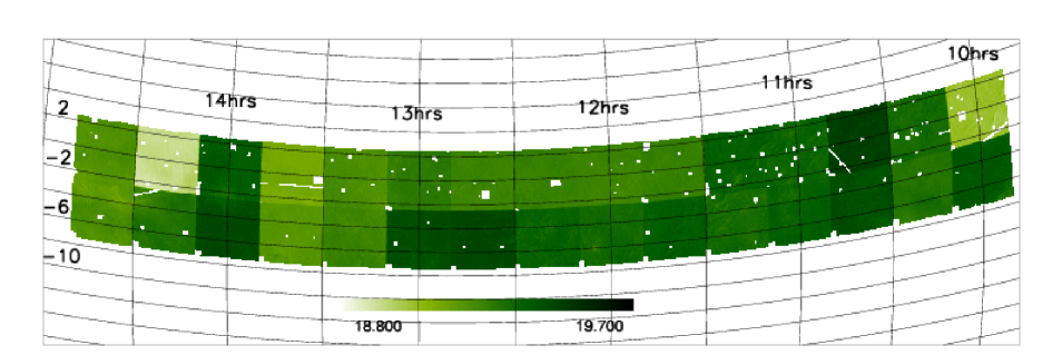
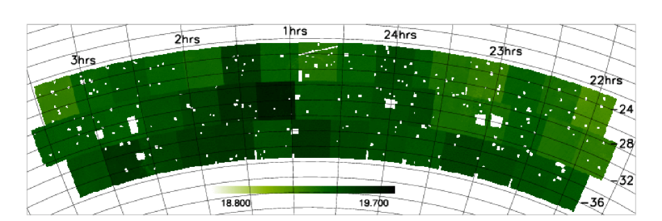
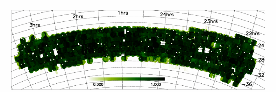
The 2dFGRS input catalogue was intended to reach a uniform extinction-corrected APM magnitude limit of ${\rm b_{J}}=19.45$. However, since the original definition of the catalogue, our understanding of the calibration of APM photometry has improved. In the preliminary 100k release (Colless et al., 2001), the APM magnitudes were directly recalibrated using CCD data from the EIS (Prandoni et al., 1999; Arnouts et al., 2001) and 2MASS (Jarrett et al., 2000) (see Norberg et al., 2002b). In the final data release it has been possible to improve the calibration still further (see Colless et al. 2003 and below). In addition, the Schlegel et al. (1998) extinction maps were finalised after the catalogue was selected; thus, the final survey magnitude limit varies with position. As described in Norberg et al. (2002b) an accurate map of the resulting magnitude limit can be constructed. Fig. 1 shows these maps for the final NGP and SGP strips of the survey. Note that the maps also serve to delineate the boundary of the survey and the regions cut out around bright stars and satellite tracks.

The improvements in the photometry derived from the UK Schmidt plates comes in part because these have been scanned using the SuperCOSMOS measuring machine (Hambly, Irwin & MacGillivray, 2001). SuperCOSMOS has some advantages in precision with respect to the APM, yielding improved linearity and smaller random errors. In a similar way to the APM survey, the SuperCOSMOS recalibration matches plate overlaps (Colless et al. 2003). The magnitudes have been placed on an absolute scale using the SDSS EDR (Stoughton et al. 2002) in 33 plates, the ESO imaging survey (e.g. Arnouts et al. 2001) in 7, plus the ESO-Sculptor survey (Arnouts et al. 1997 ).

When the SuperCOSMOS $b_{\rm\scriptscriptstyle J,SC}$ data are compared to the 2dFGRS APM photometry, there is evidence for a small non-linear term, which we eliminate by applying the correction

$${\rm b_{J}}^{\prime}={\rm b_{J}}+0.033([{\rm b_{J}}-18]^{2}-1)\quad{\rm for}\quad{\rm b_{J}}>15.5$$ (1)

and a fixed offset for ${\rm b_{J}}<15.5$. We then determine quasilinear fits of the form

$${\rm b_{J}}^{\prime\prime}=A\,{\rm b_{J}}^{\prime}+B,$$ (2)

where $A$ and $B$ are determined separately for each plate to minimize the rms difference ${\rm b_{J}}^{\prime\prime}-b_{\rm\scriptscriptstyle J,SC}$. The final 2dFGRS magnitudes, ${\rm b_{J}}^{\prime\prime}$, are given in the release database. For many purposes (e.g. defining the colour of a galaxy) the SuperCOSMOS magnitudes are the preferred choice, but for defining the survey selection function we use the final APM magnitudes as it is for these that the survey has a well defined magnitude limit.

2.2 Colour data

SuperCOSMOS has also scanned the UKST $r_{\rm\scriptscriptstyle F}$ plates (Hambly, Irwin & MacGillivray, 2001), and these have been calibrated in the same manner as the ${\rm b_{J}}$ plates. The $r_{\rm\scriptscriptstyle F}$ plates are of similar depth and quality to the ${\rm b_{J}}$ plates, giving the important ability to divide galaxies by colour.

The systematic calibration uncertainties are at the level of $0.04$ mag. rms in each band. This uncertainty is significantly smaller than the rms differences between the SuperCOSMOS and SDSS photometry ($0.09$ mag $3\sigma$ clipped rms in each band, as compared with $0.15$ mag when APM magnitudes are used). However, some of this dispersion is not a true error in SuperCOSMOS: SDSS photometry is not perfect, nor are the passbands and apertures used identical. A fairer estimate of the random errors can probably be deduced from the histogram of rest-frame colours given below in Fig. 2. This shows a narrow peak for the early-type population with a FWHM of about $0.2$ mag. If the intrinsic width of this peak is extremely narrow such that the measured width is dominated by the measurement errors this gives us an upper limit on the errors in photographic ${\rm b_{J}}-r_{\rm\scriptscriptstyle F}$ colour of $0.2/\sqrt{8\ln(2)}\approx 0.085$ mag, or an uncertainty of only $0.06$ mag in each band (including calibration systematics).

In our power spectrum analysis, we will wish to split the sample by rest frame colour so as to compare the clustering of intrinsically red and blue subsamples. To achieve this we need to be able to $k$-correct the observed colours.

2.2.1 $k$-corrections

The problem we face is this: given a redshift and an observed ${\rm b_{J}}-r_{\rm\scriptscriptstyle F}$ colour, how do we deduce a consistent $k$-correction for each band? The simplest solution is to match the colours to a single parameter, which could be taken to be the age of a single-metallicity starburst. This approach was implemented using the models of Bruzual & Charlot (2003). Their Single Stellar Populations (SSPs) vary age and metallicity, and these variations will be nearly degenerate. In practice, we assumed 0.4 Solar metallicity ($Z=0.008$) and found the age that matches the data. For very red galaxies, this can imply a current age $>13$ Gyr; in such cases an age of 13 Gyr was assumed, and the metallicity was raised until the correct colour was predicted.

In most cases, this exercise matched the results of the Blanton et al. (2003) KCORRECT package (version 3.1b), which fits the magnitude data using a superposition of realistic galaxy spectral templates. The results of Blanton et al. are to be preferred in the region where the majority of the data lie; this can be verified by taking the full DR1 $ugriz$ data and fitting $k$-corrections, then comparing with the result of fitting $gr$ only. The differences are small, but are smaller than the difference between the KCORRECT results and fitting burst models. The main case for which this matters is for the red $k$-correction for blue galaxies. However, some galaxies can be redder than the reddest template used by Blanton et al.; for such cases, the burst models are to be preferred. In fact, the two match almost perfectly at the join.

Figure 2: Photographic ${\rm b_{J}}-r_{\rm\scriptscriptstyle F}$ colour versus redshift for the 2dFGRS, as observed (top) and in the rest frame (middle). The separation between ‘early-type’ (red) and ‘late-type’ (blue) galaxies is very clear. The third panel shows the histogram of $k$-corrected restframe colours, which is very clearly bimodal. This is strongly reminiscent of the distribution of spectral type, $\eta$, and dividing the sample at a rest frame colour of $({\rm b_{J}}-r_{\rm\scriptscriptstyle F})_{z=0}=1.07$ (dotted line) achieves a very similar separation of early-type ‘class 1’ galaxies from classes 2–4, as was done using spectra by Madgwick et al. (2002).

Figure 3: Maps of the overall redshift completeness, $R(\theta)$, averaged over apparent magnitude, in the NGP and SGP strips.

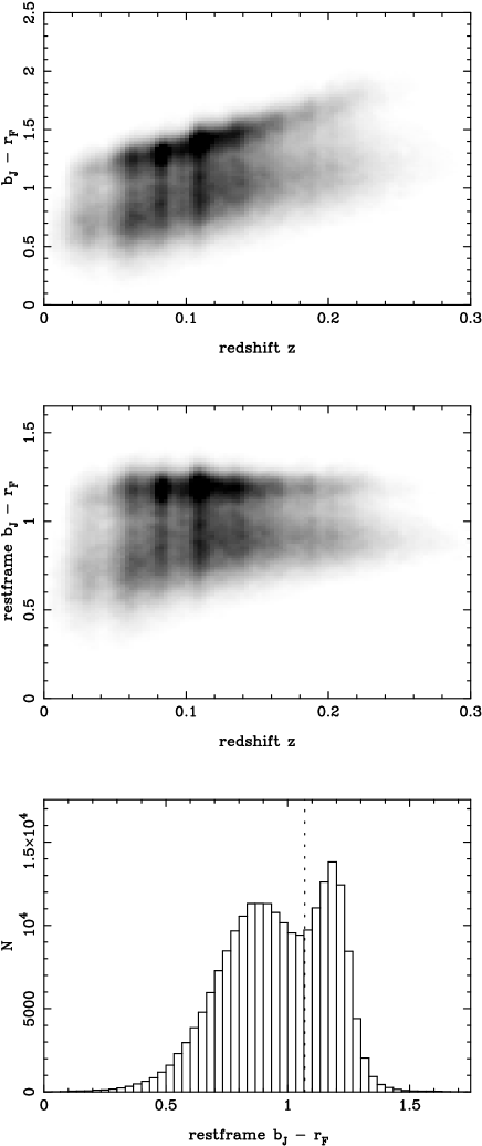
The following fitting formula, which we adopt, summarizes the results of this procedure, and is good to 0.01 mag almost everywhere in the range of interest:

  $${k_{{\rm b_{J}}}=} {{}(-1.63+4.53C)y+(-4.03-2.01C)y^{2}} {{}-z/(1+(10z)^{4})} {k_{r_{\rm\scriptscriptstyle F}}=} {{}(-0.08+1.45C)y+(-2.88-0.48C)y^{2},}$$   (3)

where $y\equiv z/(1+z)$ and $C\equiv{\rm b_{J}}-r_{\rm\scriptscriptstyle F}$. In most cases, the deviations from the fit are probably only of the order of the accuracy of the whole exercise, so they are ignored in the interests of clarity. The distributions of observed and $k$-corrected rest frame colours are shown in Fig. 2.

The histogram of rest frame colours exhibits the well known bimodal distribution (Strateva et al., 2001; Baldry et al., 2004). Related spectral quantities such as H$\delta$ absorption and the $4000\,$Angstrom break show similar bimodal distributions (Kauffmann et al., 2003). In particular, colour is strongly correlated with the 2dFGRS spectral type $\eta$ (see figure 2 of Wild et al. 2005). Thus dividing the sample at a rest frame colour of $({\rm b_{J}}-r_{\rm\scriptscriptstyle F})_{z=0}=1.07$ achieves a very similar separation of early-type ‘class 1’ galaxies from classes 2–4, as was done using spectra by Madgwick et al. (2002).

2.3 Spectroscopic completeness

Figure 4: Maps illustrating the redshift completeness at ${\rm b_{J}}=19.5$ relative to that at bright magnitudes. The magnitude dependence of this redshift completeness is assumed to be proportional to $1-\exp({\rm b_{J}}-\mu)$ and the parameter $\mu$ is estimated for each sector in the survey mask. Here, we plot the factor $1-\exp({\rm b_{J}}-\mu)$ for a fiducial magnitude of ${\rm b_{J}}=19.5$.

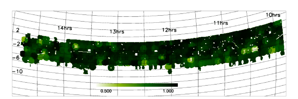
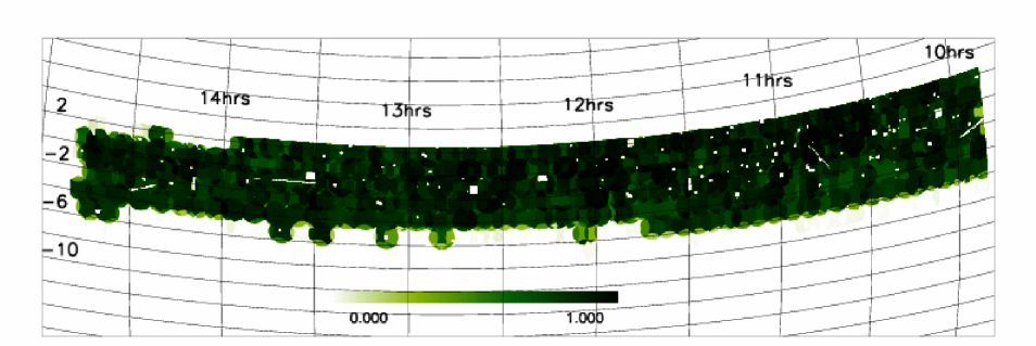
The spectroscopic completeness, the fraction of 2dFGRS galaxies with reliably measured redshifts, varies across the survey. This can be due to a failure to measure redshifts from the observed spectra or to whole fields missing, either because they were never observed, or because they were rejected when they had unacceptably low spectroscopic completeness. In addition, there is a small level of incompleteness arising from galaxies that were never targeted due to restrictions in fibre positioning. In the samples we analyse we reject all fields (single observations) that have a spectroscopic completeness less than 70%. As the observed 2dF fields overlap in a complex pattern, the completeness varies from sector to sector, where a sector is defined by a unique set of overlapping fields. Maps of the redshift completeness, $R(\theta)$, of the final survey, constructed as detailed in Norberg et al. (2002b), are shown in Fig. 3. Here $\theta$ denotes the angular position on the sky. For the two main survey strips, 80% of the area has a completeness greater than 80%.

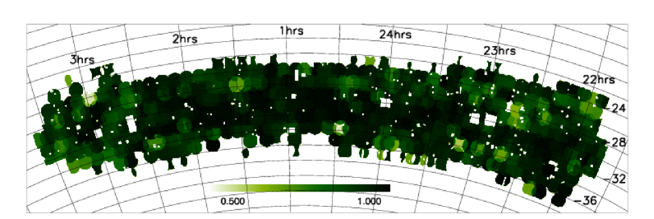
In observed fields, the fraction of galaxies for which useful (quality $\geq 3$) redshifts have not been obtained increases significantly with apparent magnitude. In Norberg et al. (2002b) (see also Colless et al., 2001), we define an empirical model of this magnitude dependent incompleteness. In this model, the fraction of observed galaxies yielding useful redshifts is proportional to $1-\exp({\rm b_{J}}-\mu)$ and, by averaging over fields, the parameter $\mu$ is defined for each sector in the survey. Fig. 4, shows a map of the factor $1-\exp({\rm b_{J}}-\mu)$ for a fiducial apparent magnitude of ${\rm b_{J}}=19.5$. For a given apparent magnitude and position the overall redshift completeness is given by the product

$$C(\theta,{\rm b_{J}})=A(\theta)R(\theta)[1-\exp({\rm b_{J}}-\mu)],$$ (4)

where $R(\theta)$ and $[1-\exp({\rm b_{J}}-\mu)]$ are the quantities illustrated in Figs 3 and 4. In each sector, we define the normalizing constant $A(\theta)=\langle[1-\exp({\rm b_{J}}-\mu(\theta))]\rangle^{-1}$ averaged over the expected apparent magnitude distribution of survey galaxies, so that $\langle C(\theta,{\rm b_{J}})\rangle=R(\theta)$. In general, this magnitude dependent incompleteness is not a large effect. At the magnitude limit of the survey, 50%(80%) of the survey’s area has completeness factor, $[1-\exp({\rm b_{J}}-\mu)]$, greater than 88%(80%).

Since it is easier to measure the redshift of blue emission line galaxies than of red galaxies, we expect the level of incompleteness to be different for our red and blue subsamples. Since we are unable to classify a galaxy by rest frame colour without knowing its redshift, it is not trivial to estimate the level of incompleteness in each subsample. However, to a first approximation, we can quantify the incompleteness as a function of the observed colour. In fact, we can do better than this by noting that our red and blue subsamples are quite well separated on a plot of observed colour versus apparent magnitude. We can split the galaxies in this plane into two disjoint samples. Quantifying the incompleteness for red and blue subsamples split in this way we find they are again reasonably well fit by the model $1-\exp({\rm b_{J}}-\mu)$, but with $\mu_{\rm blue}=\mu+0.65$ and $\mu_{\rm red}=\mu-0.25$. These are values we use in Section 5.3, where we compare the power spectra of the red and blue galaxies.

3 Luminosity function and evolution

Table 1: The parameters of the Schechter luminosity functions and $k+e$ corrections (see equation 7) that define the standard model of the survey selection function. Two Schechter functions are combined to describe the luminosity function of red galaxies.

	$\Phi^{*}/{\rm h^{3}Mpc}^{-3}$	$M^{*z=0.1}_{\rm b_{J}}-5{\log_{10}h}$	$\alpha$	$a$	$b$	$c$
Combined	0.0156	$-19.52$	$-1.18$	0.327	6.18	10.3
Blue	0.00896	$-19.55$	$-1.3\hphantom{0}$	0.282	5.67	31.1
Red	0.00909	$-19.19$	$-0.5\hphantom{0}$	1.541	6.78	7.95
	0.00037	$-19.87$	$-0.5\hphantom{0}$	1.541	6.78	7.95

For a complete understanding of how the 2dFGRS probes the universe, we need to supplement the selection masks described above with a model for the galaxy luminosity function. It will also be necessary to understand how the luminosity function depends on galaxy type and how it evolves with redshift.

In Norberg et al. (2002b), we demonstrated that a Schechter function was a good description of the overall 2dFGRS luminosity function and we estimated a mean $k+e$ correction by fitting Bruzual & Charlot (1993) population synthesis models to a subset of the 2dFGRS galaxies for which SDSS $g-r$ colours were available. Repeating this procedure for the recalibrated final 2dFGRS magnitudes yields a Schechter function with $\alpha=-1.18$, $\Phi^{*}=1.50\times 10^{-2}\,h^{3}{\rm Mpc^{-3}}$, $M^{*z=0.1}_{{\rm b_{J}}}-5\log_{10}h=-19.57$, where we have quoted the characteristic absolute magnitude at the median redshift of the survey, $z=0.1$, $M^{*z=0.1}_{{\rm b_{J}}}\equiv M^{*z=0}_{{\rm b_{J}}}+k(z=0.1)+e(z=0.1)$ rather than the redshift $z=0$ value. Since our purpose is to model only those galaxies that are in the 2dFGRS, we have ignored the 9% boost to $\Phi^{*}$ that was applied in Norberg et al. (2002b) to compensate for incompleteness in the 2dFGRS input catalogue. Thus, the corresponding values from Norberg et al. (2002b) are $\alpha=-1.21\pm 0.03$, $\Phi^{*}=(1.47\pm 0.08)\times 10^{-2}\,h^{3}{\rm Mpc^{-3}}$, $M^{*z=0.1}_{{\rm b_{J}}}-5\log_{10}h=-19.50\pm 0.07$. The $1$-$\sigma$ shifts in $\alpha$ and $M^{*}_{{\rm b_{J}}}$ are systematic changes resulting from the photometric recalibration. The uncertainties on each of these parameters remain essentially unchanged. The luminosity functions determined separately in the NGP, SGP and RAN field regions agree extremely well in shape, but are slightly offset in $M^{*}_{{\rm b_{J}}}$. In the standard calibration used in this paper we apply a shift of $-0.0125$ in the SGP and $0.022$ in the NGP to the galaxy magnitudes and magnitude limits to make all the regions consistent with the luminosity function estimated from the full survey, but as we shall see, these shifts are so small that they make very little difference.

Figure 5: The solid curves in the upper panel show stepwise estimates of the overall 2dFGRS luminosity function and estimates for red and blue subsets, split at a restframe colour of ${\rm b_{J}}-r_{\rm\scriptscriptstyle F}=1.07$. They are plotted as a function of absolute magnitude at $z=0.1$, which we define in terms of $z=0$ absolute magnitude as $M^{*z=0.1}_{{\rm b_{J}}}\equiv M^{*z=0}_{{\rm b_{J}}}+k(z=0.1)+e(z=0.1)$. The smooth dashed curves are Schechter functions convolved with the model of the magnitude measurement errors. It is these luminosity functions that are used to construct random unclustered galaxy catalogues. The corresponding maximum likelihood estimates of the $k+e$ corrections (relative to their values at $z=0.1$) are shown by the solid curves in the lower panel. The long-dashed line in the upper panel is an STY estimate of the overall luminosity function when the $k+e$ correction shown as the long-dashed line in the lower panel is adopted.

The main problem with the previous procedure was that the evolution is assumed to be known. Here, we take the safer approach of estimating empirical $k+e$ corrections directly from the data. If we model the luminosity function by a function $\phi(L)$ of the $k+e$ corrected luminosity $L$, and the radial density field by a function of redshift $\rho(z)$, then following Saunders et al. (1990) we can define the joint likelihood as

$${\cal L}_{1}=\frac{\Pi_{i}\,\rho(z_{i})\phi(L_{i})}{\int\!\!\!\int\rho(z)\phi(L)\frac{dV}{dz}\,dL\,dz},$$ (5)

where the product is over the galaxies in the sample. Note for convenience one can select from the 2dFGRS a simple magnitude limited subsample. At each redshift, the range of the luminosity integral in the denominator is determined by the apparent magnitude limits and the model $k+e$ correction. One could then parameterize $\phi(L)$, $\rho(z)$ and $k(z)+e(z)$ and seek their maximum likelihood values. In practice, this does not work well for our data as, without a constraint on $\rho(z)$, there is a near degeneracy between $k+e$ and the faint end slope of the luminosity function. This problem can be removed by introducing an additional factor into the likelihood to represent the probability of observing a given $\rho(z)$. Estimating this probability using the randomly distributed clusters model of Neyman & Scott (1952) (see also Peebles, 1980), the likelihood becomes

$${\cal L}={\cal L}_{1}\ \times\ \Pi_{r}\,\exp\left(-\frac{1}{2}\frac{(\rho(z_{r})/\bar{\rho}-1)^{2}N_{r}}{(1+4\pi J_{3}N_{r}/V_{r})}\right).$$ (6)

Here $\rho(z_{r})$, $N_{r}$ and $V_{r}$ are respectively the galaxy density, number of galaxies and comoving volume of the $r^{\rm th}$ radial bin. The overall mean galaxy density is $\bar{\rho}$ and $J_{3}$ is the usual integral over the two-point correlation function. We adopt $J_{3}=400\,({\,h^{-1}\,\rm Mpc})^{3}$, consistent with the measured 2dFGRS correlation function (Hawkins et al., 2003).

Note that when splitting the sample into the two colour classes we ignore any evolutionary correction to their colours. This cannot be exactly correct, but at the quite red dividing colour of ${\rm b_{J}}-r_{\rm\scriptscriptstyle F}=1.07$, galaxies are not star forming and the evolutionary colour correction is expected to be small. This approximation is supported empirically by the central panel of Fig. 2, which shows that the rest-frame colour corresponding to the division between the red and blue populations appears to be independent of redshift.

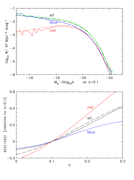
The luminosity functions and corresponding $k+e$ corrections that result from applying this method are shown in Fig. 5. Note that to model the selection function all that we require is the combined $k+e$ correction for the red and blue components of the luminosity function. Thus for modelling the selection function we do not make use of the colour dependent $k$-corrections derived in Section 2.2.1 . To utilise these would require a bivariate model of the galaxy luminosity function so that ${\rm b_{J}}-r_{\rm\scriptscriptstyle F}$ colours could be assigned to each model galaxy. We have used a stepwise parameterization of the luminosity function and assumed $k+e$ corrections of the form

$$k+e=\frac{az+bz^{2}}{1+cz^{3}},$$ (7)

where $a$, $b$ and $c$ are constants. The solid lines in the upper panel show the luminosity function estimates for the full sample and for the red and blue subsets. The solid curves in the lower panel show the corresponding maximum likelihood $k+e$ corrections. For the purpose of constructing unclustered galaxy catalogues it is useful to fit these estimates using Schechter functions convolved with the measured distribution of magnitude errors from Norberg et al. (2002b). The smooth dashed curves that closely match each of the maximum likelihood estimates are these convolved Schechter functions. In the case of the red galaxies we have used the sum of two Schechter functions to produce a sufficiently good fit. The parameters of these Schechter functions and the corresponding $k+e$ correction parameters are listed in Table 1.

These luminosity functions can be compared with those of Madgwick et al. (2002), who estimated the luminosity functions of 2dFGRS galaxies classified by spectral type using a principal component analysis. Although there is not a one-to-one correspondence between colour and spectral class, our red sample corresponds closely to their class 1 and our blue sample to the combination of the remaining classes 2, 3 and 4. The shape and normalization of our luminosity functions agree well: the only difference occurs fainter than $M_{{\rm b_{J}}}>-16$, where for the earliest spectral type, Madgwick et al. (2002) find an excess over a Schechter function which is not apparent in our red sample. At first sight, the values of $M^{*}$ and hence the positions of the bright end of the luminosity functions appear to differ. Madgwick et al. (2002) find that late type galaxies have significantly fainter $M^{*}$ than early types, while the bright ends of our blue and red luminosity functions are very close. This apparent difference is because Madgwick et al. correct their luminosity functions to $z=0$ while our estimates are for a fiducial redshift of $z=0.1$. In addition, Madgwick et al. apply only $k$-corrections while our modelling also includes mean $e$-corrections for each class. Because the $k+e$ corrections for the red (early) galaxies are much greater than for the blue (late) galaxies this brings the $M^{*}$ values at $z=0.1$ much closer together. In fact, we find a very good match with the Madgwick et al. (2002) results once the difference in $k+e$ corrections is accounted for and the results translated to $z=0.1$.

We also compare the overall luminosity function and mean $k+e$ correction with the result of applying the method we used previously in Norberg et al. (2002b). For this purpose, we adopt $k+e=(z+6z^{2})/(1+8.9z^{2.5})$, which is shown by the long-dashed line in the lower panel of Fig. 5. This is essentially identical to the fit used in Norberg et al. (2002b). The luminosity function estimated using the STY method, again convolved with the same model for the magnitude errors, is shown by the long dashed line in the upper panel. We note that apart from $z<0.05$, where there are relatively few 2dFGRS galaxies, this $k+e$ correction is in good agreement with our new maximum likelihood estimate. Similarly, the luminosity function is in quite close agreement with our new estimate for the combined red and blue sample.

3.1 Random unclustered catalogues

Armed with realistic luminosity functions and evolution corrections, plus an accurate characterization of survey masks, we can now generate corresponding random catalogues of unclustered galaxies (not to be confused with the RAN data from the randomly-placed 2dFGRS survey fields). The procedure we adopt to do this is as described in Section 5 of Norberg et al. (2002b), except that we now have the option of treating the red and blue subsamples separately. In this procedure, we perturb the magnitude and redshifts in accordance with the known measurement errors. The mock catalogues include a number of properties in addition to the angular position, apparent magnitude and redshift of each galaxy:

• The overall redshift completeness, $c_{i}$, in the direction of each galaxy, as given by the completeness measure described in Section 2.3.

• The mean expected galaxy number density $n_{i}$ at each galaxy’s position, taking account of the survey magnitude limit in this direction, and the dependence of redshift completeness on apparent magnitude as characterized by the parameter $\mu$.

• The expected bias parameter $b_{i}$ of a galaxy of a given luminosity and colour as defined by the simple model in Section 4.1.

Note that when the red and blue subsamples are analysed separately, $n_{i}$ refers only to galaxies of the same colour class, but if the random catalogue is to be used in conjunction with the full 2dFGRS catalogue, then $n_{i}$ is defined in terms of a sum over contributions from both the red and blue subsamples. The value of this parameter will also vary if one places additional cuts on the catalogue such as varying the faint magnitude limit. As we shall see in Section 4.1, these quantities are useful when estimating the galaxy power spectrum.

Figure 6: The histograms in the top panel show the redshift distribution of the 2dFGRS data in the SGP, NGP and RAN field regions. The curves show the distribution in the corresponding random unclustered catalogues. The lower panel shows the same distributions, but weighted with a redshift dependent function as in the power spectrum analysis, using $J_{3}=400$ h^-3Mpc³. In all cases, the histograms for the random catalogues are normalized so that the sum of the weights matches that of the corresponding data.

Figure 7: As Fig. 6 but for the red subset with rest frame colours redder than $({\rm b_{J}}-r_{\rm\scriptscriptstyle F})_{z=0}>1.07$.

Figure 8: As Fig. 6 but for the blue subset with rest frame colours bluer than $({\rm b_{J}}-r_{\rm\scriptscriptstyle F})_{z=0}<1.07$.

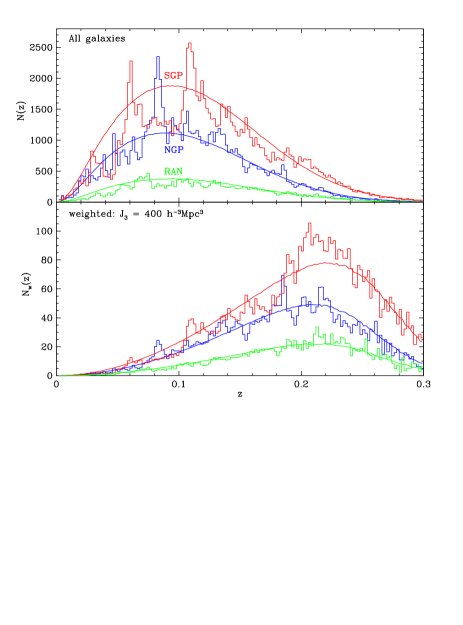
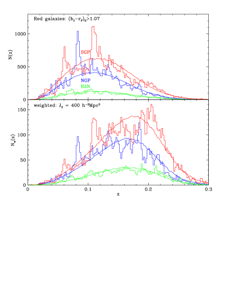
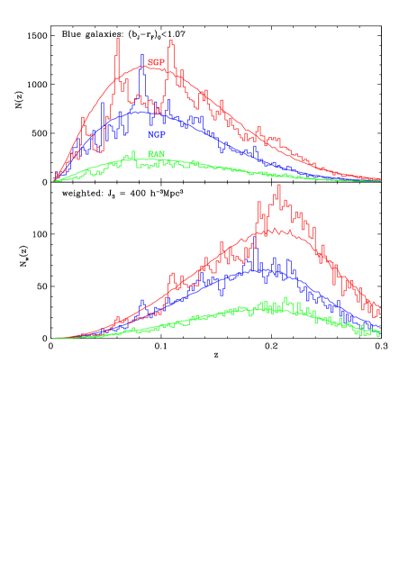
Fig. 6 compares the redshift distribution of the genuine 2dFGRS data with that of the random catalogues. The upper panel shows the number of galaxies, binned by redshift, that pass the selection criteria defining the samples used in the power spectrum analysis. The lower panel shows the same distributions but weighted by the radial weight that is used in the power spectrum analysis. Figs 7 and 8 repeat this comparison for the red and blue subsets. For the NGP and RAN fields the smooth redshift distributions of the random catalogues match quite accurately the mean values for the full dataset and for the red and blue subsamples all the way to the maximum redshift of our samples ($z=0.3$). The SGP exhibits greater variation and in particular is underdense compared to the random catalogue at $z\la 0.06$. This local underdensity in the SGP has been noted and discussed many times before (e.g. Maddox et al., 1990; Metcalfe, Fong & Shanks, 1995; Frith et al., 2003; Busswell et al., 2004). In discussing the 2dFGRS 100k data, Norberg et al. (2002b) demonstrated, in their figures 13 and 14, that similar redshift distributions were not unexpected in $\Lambda$CDM mock catalogues. Moreover, the lower panels in Figs 6,  7 and 8, which weight the galaxies in the same way as in the power spectrum analysis, indicate that the contribution from this local region is negligible. With this weighting, it is the excess in the SGP at $0.2<z<0.24$ that appears more prominent. This excess appears to be due to two large structures around ${\rm RA}=23^{\rm h}$ and $2^{\rm h}$. It is therefore likely that these excursions are due to genuine large scale structure. Nevertheless, in Section 6.6 we assess the sensitivity of our power spectrum estimate to the assumed redshift distribution by also considering an empirical redshift distribution.

4 Power spectrum estimation and error assignment

4.1 The power spectrum estimator

We employ the Fourier based method of Percival, Verde & Peacock (2004a; PVP) which is a generalization of the minimum variance method of Feldman, Kaiser & Peacock (1994; FKP) to the case where the galaxies have a known luminosity and/or colour dependent bias. This procedure requires an assumed cosmological geometry in order to convert redshifts and positions on the sky to comoving distances in redshift space. Strictly, this geometry should vary with the cosmological model being tested. However, the effect of such a change is very small (this was extensively tested in P01). We have therefore simply assumed a cosmological model with $\Omega_{\rm m}=0.3$ and $\Omega_{\Lambda}=0.7$ for this transition.

In our implementation, we carry out a summation over galaxies from the data and random catalogues to evaluate the weighted density field

$$F({\bf r})=\frac{1}{N}\int\frac{w({\bf r},L)}{b(L)}\,\left[{n_{\rm L}^{\rm g}}({\bf r},L)-\alpha{n_{\rm L}^{\rm r}}({\bf r},L)\right]\,dL$$ (8)

on a cubic grid. Here ${n_{\rm L}^{\rm g}}({\bf r},L)$ and ${n_{\rm L}^{\rm r}}({\bf r},L)$ are the number density of galaxies of luminosity $L$ to $L+dL$ at position ${\bf r}$ in the data and random catalogues respectively. It is straightforward to generalize this to include a summation over galaxies of different types or colours. Early analysis of the 2dFGRS found a bias parameter of $b\approx 1$ (Verde et al., 2002; Lahav et al., 2002) for $L_{*}$ galaxies averaged over all types. Subsequently we have determined that the bias parameter depends both on luminosity and galaxy type or colour. Here we adopt a scale independent bias parameter

$$b(L)=0.85+0.15(L/L_{*}),$$ (9)

as found by Norberg et al. (2001). For red and blue subsets, split by a rest frame colour of $({\rm b_{J}}-r_{\rm\scriptscriptstyle F})_{z=0}=1.07$, the bias is significantly different and we adopt

$$b_{\rm red}=1.3\,[0.85+0.15(L/L_{*})]$$ (10)

and

$$b_{\rm blue}=0.9\,[0.85+0.15(L/L_{*})],$$ (11)

which, as we find in Section 5.3, empirically describes the difference in amplitudes of the power spectra of red and blue galaxies around $k=0.1{\,h\,\rm Mpc^{-1}}$. Note that in all these formulae the $L_{*}$ refers to the Schechter function fit to the overall 2dFGRS luminosity function.

The minimum variance weighting function is given by (PVP)

$$w({\bf r},L)=\frac{b^{2}(L)\,w^{\rm A}({\bf r})}{1+4\pi(J_{3}/b^{2}_{\rm T})\int b^{2}(L^{\prime})\,{{\bar{n}}_{\rm L}^{\rm g}}({\bf r},L^{\prime})\,dL^{\prime}}.$$ (12)

Here ${{\bar{n}}_{\rm L}^{\rm g}}({\bf r},L^{\prime})$ ($\equiv\alpha{{\bar{n}}_{\rm L}^{\rm r}}({\bf r},L^{\prime})$) is the expected mean density of galaxies of luminosity $L^{\prime}$ at position ${\bf r}$ in the survey. Our standard choice for $J_{3}$ is $400\,h^{-3}$Mpc³ and refers to the value for typical galaxies in the weighted 2dFGRS, for which the typical bias factor relative to that of $L_{*}$ galaxies is $b_{\rm T}=1.26$. To revert to the standard weighting function for the FKP estimator, we replace $b(L)$ by $b_{\rm T}$. The weighting function, $w({\bf r},L)$, takes account of the galaxy luminosity function, varying survey magnitude limits, varying completeness on the sky and its dependence on apparent magnitude. The angular weight $w^{\rm A}({\bf r})$ has a mean of unity and gives a statistical correction for missing close pairs of galaxies caused by fibre placing constraints (see Section 6.3 for details).

The factor $\alpha$ in (8) is related to the ratio of the number of galaxies in the random catalogues to that in the real galaxy catalogue. It is defined as

$$\alpha=\frac{\int\!\!\!\int\frac{w({\bf r},L)}{b(L)}\,{n_{\rm L}^{\rm g}}({\bf r},L)\,dL\,d^{3}{\bf r}}{\int\!\!\!\int\frac{w({\bf r},L)}{b(L)}\,{n_{\rm L}^{\rm r}}({\bf r},L)\,dL\,d^{3}{\bf r}},$$ (13)

which reduces to a sum over the real and random galaxies

$$\alpha=\sum_{\rm data}\frac{w_{i}}{b_{i}}\;\Big{/}\,\sum_{\rm random}\frac{w_{i}}{b_{i}}.$$ (14)

Similarly, the constant $N$ in (8), which normalizes the survey window function, is defined as

$$N^{2}\equiv\int\left[\int{{\bar{n}}_{\rm L}^{\rm g}}({\bf r},L)w({\bf r},L)dL\right]^{2}d^{3}{\bf r},$$ (15)

which can be written as a sum over the random galaxies

$$N^{2}=\alpha\sum_{\rm random}{{\bar{n}}^{\rm g}}_{i}w_{i}^{2},$$ (16)

where ${{\bar{n}}^{\rm g}}_{i}$ is the expected mean galaxy density at the position of the $i$th galaxy in the random catalogue. This quantity is evaluated and tabulated at the position of each galaxy so that we can use this simple summation to evaluate $N^{2}$.

To evaluate $F({\bf r})$ we loop over real and random galaxies, calculate their spatial positions assuming a flat $\Omega_{\rm m}=0.3$ cosmology, and use cloud-in-cell assignment (e.g. Efstathiou et al., 1985) to accumulate the difference in $(w_{i}/b_{i})_{\rm data}-\alpha(w_{i}/b_{i})_{\rm random}$ on a grid. We first do this with a $256^{3}$ grid in a cubic box of $L^{0}_{\rm box}=3125{\,h^{-1}\,\rm Mpc}$. Periodic boundary conditions are applied to map galaxies whose positions lie outside the box. To obtain estimates at smaller scales we repeat this with $256^{3}$ grids of size $L_{\rm box}=L^{0}_{\rm box}/4$, $L^{0}_{\rm box}/16$. We then use an FFT to Fourier transform these fields and explicitly correct for the smoothing effect of the cloud-in-cell assignment (e.g. Hockney & Eastwood, 1981, chap. 5). From each grid we retain only estimates for $k<0.63\,k_{\rm Nyquist}$, where the correction for the effects of the grid are highly accurate. Thus, from the largest box we sample the power spectrum well on a 3D grid of spacing $dk\simeq 0.002{\,h\,\rm Mpc^{-1}}$ covering $0.002<k<0.16{\,h\,\rm Mpc^{-1}}$. The smaller boxes give a coarse sampling of the power spectrum with resolutions of $dk=0.008$ and $0.032{\,h\,\rm Mpc^{-1}}$ well into the non-linear regime $0.16<k<2.5{\,h\,\rm Mpc^{-1}}$, where our estimates become shot noise limited.

The shot noise corrected power spectrum estimator is

$$\hat{P}({\bf k})=\langle|F({\bf k})|^{2}\rangle-P_{\rm shot},$$ (17)

where $P_{\rm shot}=S/N^{2}$ with

$$S\equiv\sum_{\rm data}\frac{w_{i}^{2}}{b_{i}^{2}}+\alpha^{2}\sum_{\rm random}\frac{w_{i}^{2}}{b_{i}^{2}}.$$ (18)

Finally, we average the power over direction, in shells of fixed $|{\bf k}|$ in redshift space.

The power spectrum, $\hat{P}(k)$, is an estimate of the true underlying galaxy power spectrum convolved with the power spectrum of the survey window function,

$$W({\bf r})=\frac{\alpha}{N}\int w({\bf r},L)\,{n_{\rm L}^{\rm r}}({\bf r},L)\,dL.$$ (19)

Thus, to model our results we also need an accurate estimate of the window function. This we obtain using the same techniques as above. The normalization is such that $\int W^{2}({\bf k})\;d^{3}{\bf k}=1$. Under the approximation that the underlying power spectrum is isotropic, i.e. ignoring redshift distortions, then the operations of spherical averaging and convolving commute. In Section 4.2.3 we test the effect of redshift distortions via direct Monte Carlo simulations using the Hubble volume mock catalogues described in Section 4.2.1. Thus, all that we require is a model of the spherically averaged window function. The curve going through the filled circles in Fig. 9 shows the window function that results for our standard choice of data cuts and weights. The window function marked by the open circles results from removing the random fields. This comparison shows that the secondary peak in the window function of our standard dataset is due to the discrete random 2 degree fields. Also shown, as the dashed line, is the window function computed for the smaller 100k sample in P01.

Figure 9: The amplitude of the spherically averaged 2dFGRS window function of our standard weighted dataset in Fourier space (filled circles). The solid line passing through these symbols gives a cubic spline (Press et al., 1992) fit to these data and was used to perform the spherical convolution of model power spectra. For comparison, we plot the window function and spline fit that results from excluding the random fields (open circles). Also the dashed line shows the fit used in Percival et al. (2001; P01), which ignores the structure in the window for $k>0.02{\,h\,\rm Mpc^{-1}}$.

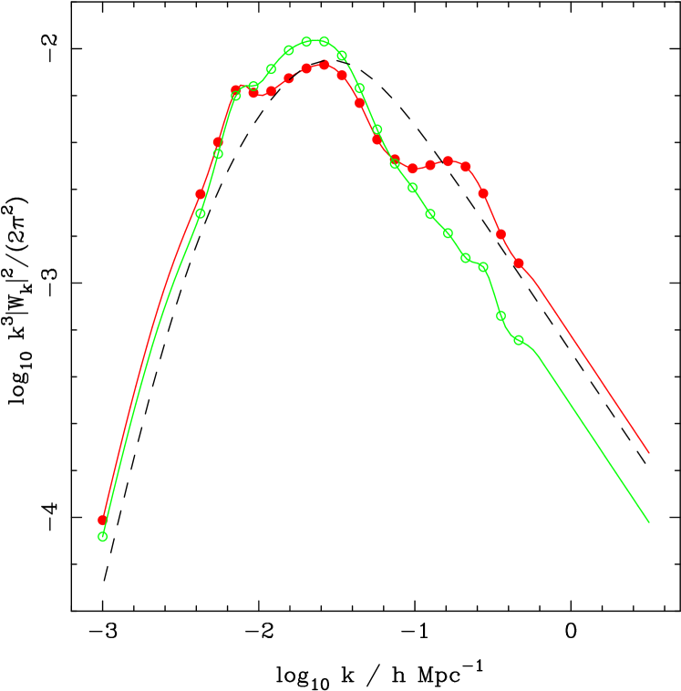
We use a 2-step process to compute the effect of this window on the recovered power spectrum. Firstly we interpolate the measured window function using a cubic spline (Press et al., 1992); examples of these interpolated window functions are shown by the solid lines in Fig. 9. Secondly, we use a modified Newton-Cotes integration scheme to perform a spherical integration numerically using this fit and determine the $k$-distribution of power required for each data point. This integration is performed once, with the result stored in a ‘window matrix’ giving the contribution from each of 1000 bins linearly spaced in $0<k<2{\,h\,\rm Mpc^{-1}}$ to each measured $P(k)$ data point. We have performed numerical integrations with fixed convergence limits for a number of power spectra, and find results similar to those calculated using this matrix. The effect of the 2dFGRS window on the recovered power is demonstrated in the next Section using mock catalogues.

4.2 Mock catalogues

To determine the statistical error in our power spectrum estimates and also to test our codes thoroughly, we employ two sets of mock catalogues.

4.2.1 Hubble volume mocks

The first set of mock catalogues are based on the $\Lambda$CDM Hubble Volume cosmological N-body simulation (Evrard et al., 2002). The Hubble Volume simulation contained $10^{9}$ particles in a box of comoving size $L_{\rm box}=3000{\,h^{-1}\,\rm Mpc}$ with cosmological parameters $h=0.7$, $\Omega_{\rm m}=0.3$, $\Omega_{\Lambda}=0.7$, $\Omega_{\rm b}=0.04$ and $\sigma_{8}=0.9$ . The galaxies are biased with respect to the mass. This is achieved by computing the local density, $\delta_{\rm s}$, smoothed with a Gaussian of width $r_{\rm s}=2{\,h^{-1}\,\rm Mpc}$, around each particle in the simulation and selecting the particle to be a galaxy with a probability

$$P(\delta_{\rm{}_{s}})\propto\cases{\exp(0.45\,\delta_{\rm s}-0.14\,\delta_{\rm s}^{3/2})&$\delta_{\rm{}_{s}}\geq 0$\cr\exp(0.45\,\delta_{\rm s})&$\delta_{\rm{}_{s}}<0$}$$ (20)

(Cole et al., 1998). The constants in this expression were chosen to produce a galaxy correlation function matching that of typical galaxies in the 2dFGRS. This can be seen in figure 6 of Hawkins et al. (2003) as in this analysis of the 2dFGRS correlation function we used the same set of 22 mock catalogues. They were also used in the analysis of the dependence of the correlation function on galaxy type and luminosity (Norberg et al., 2001, 2002a) and when analysing higher order counts in cells statistics (Baugh et al., 2004; Croton et al., 2004).

The attractive features of the Hubble Volume mocks are that their clustering properties are a good match to that of 2dFGRS and that they are fully non-linear: their density field is appropriately non-Gaussian and they have realistic levels of redshift space distortion. The limitations are that they lack luminosity or colour dependent clustering and that the 22 simulations are too few to determine the power covariance matrix accurately. We could generate more catalogues, but given the finite volume of the Hubble Volume simulation this would be of little value as they are not strictly independent.

4.2.2 Log-normal mocks

For an accurate determination of the covariance matrix of our power spectrum estimates, we need sets of mock catalogues with of order 1000 realizations. In P01, we achieved this by generating realizations of Gaussian random fields. Here, we slightly improve on this method by generating fields of a specified power spectrum with a log-normal 1-point distribution function. The log-normal model (Coles & Jones, 1991) is known to match both the results of large scale structure simulations (Kayo, Taruya & Suto, 2001) and agree empirically with 1-point distribution function of the 2dFGRS galaxy density field on large scales (Wild et al., 2005). The power spectrum we adopted for these mocks was generated using the Eisenstein & Hu (1998) algorithm with cosmological parameters $\Omega_{\rm m}h=0.168$ and $\Omega_{\rm b}/\Omega_{\rm m}=0.17$. The normalization we chose corresponds to $\sigma_{8}^{\rm gal}=0.89$ for $L_{*}$ galaxies and $\sigma_{8}^{\rm gal}=1.125$ for the typical galaxy in our weighted 2dFGRS catalogue. The method for constructing the log-normal field and random galaxy catalogue is similar to that described by PVP.

We generate a log-normal field with the required power spectrum in a cuboid aligned with the principal axes of the 2dFGRS. We have chosen to use a cuboid of dimensions $3125\times 1565.25\times 3125{\,h^{-1}\,\rm Mpc}$ covered by a grid of $512\times 256\times 512$ cubic cells. To convert this field into a mock catalogue we simply loop over all the galaxies in our random catalogue, determine which cell they occupy (applying periodic boundary conditions if necessary) and select the galaxy according to a Poisson probability distribution. The mean of the Poisson distribution is modulated by the amplitude of the log-normal field and normalized to achieve the right overall number of galaxies in the mock catalogue.

These catalogues are computationally cheap, so we can generate sufficient realizations to determine the power covariance matrix accurately. Also, by modulating the rms amplitude of the log-normal field we can build in luminosity and colour dependent clustering. Their limitations are that they are restricted to quite large scales, the level of non-Gaussianity is not necessarily realistic and they have no redshift space distortion. We assess these shortcomings by comparison to the Hubble Volume mocks.

Figure 10: Comparison of the recovered and input power spectra for a set of log-normal mocks. The two curves in the upper panel show the model input power spectrum (dashed) and its convolution with the window function of the catalogue (solid). The mean recovered power spectrum from a set of 1000 mocks and the rms scatter about this mean are shown by the points and error bars. In the lower panel, instead of using a logarithmic scale we plot, on a linear scale, the ratio of the three power spectra of the top panel to a reference model with $\Omega_{\rm m}h=0.2$ and $\Omega_{\rm b}=0$. The line types and symbols have the same meaning as in the upper panel.

Figure 11: Comparison of the expected and recovered power spectra for the Hubble Volume mock catalogues. For mocks constructed using both real-space and redshift-space galaxy positions, we compare the input non-linear power spectrum (curves) with the mean recovered power spectrum (error bars). Unlike Fig. 10, the error bars here indicate the error in the mean recovered power, computed assuming the 22 mocks to be independent. The lower panel shows, on a linear scale, these same two power spectra but divided by the same reference model as in Fig. 10 with $\Omega_{\rm m}h=0.2$ and $\Omega_{\rm b}=0$. Also shown as filled circles in the lower panel is the estimated power from the 22 mock catalogues in redshift space but after applying the cluster collapsing algorithm. These match the redshift-space estimates on large scales but have more power on small scales.

4.2.3 Analysis of mock catalogues

We now apply the method for estimating the power spectrum, described in Section 4.1, to our two sets of mock catalogues. This exercise allows us to test our code, illustrate the effect of the window function and assess the level of systematic error that results from ignoring the anisotropy of the redshift space power spectrum.

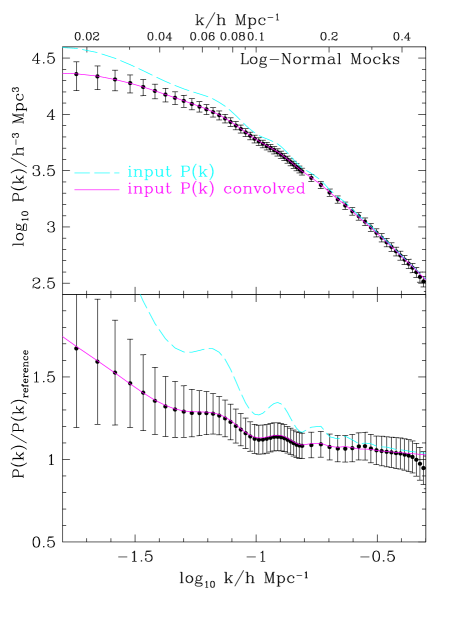
Fig. 10 compares power spectrum estimates from the log-normal mocks with the input power spectrum. These mocks have clustering that depends on luminosity according to equation 9 and are analysed using the PVP method assuming the same dependence of bias parameter on luminosity. The dashed curve shows the intrinsic input power spectrum and the solid curve the result of convolving it with the survey window function. In the lower panel one sees that the baryon oscillations present in the input power spectrum are greatly suppressed by the convolution with the window function. The points with error bars show the mean recovered power spectrum and the rms scatter about the mean for a set of 1000 mocks. We see that for $k<0.4{\,h\,\rm Mpc^{-1}}$ the mean recovered power is in excellent agreement with the convolved input spectrum. In particular, there is no perceptible glitch in the recovered power at $k=0.16{\,h\,\rm Mpc^{-1}}$ where we switch between the $3125$ and $781.25{\,h^{-1}\,\rm Mpc}$ boxes used for the FFTs. The PVP method has correctly recovered the input power spectrum with no biases due to the luminosity dependence of the clustering. At the edge of the plots, as we approach the Nyquist frequency, $k_{\rm ny}=0.51{\,h\,\rm Mpc^{-1}}$, of the grid on which the log-normal field was generated, the recovered power begins to deviate significantly from input power. For $k>0.4{\,h\,\rm Mpc^{-1}}$ our log-normal mocks are of limited value.

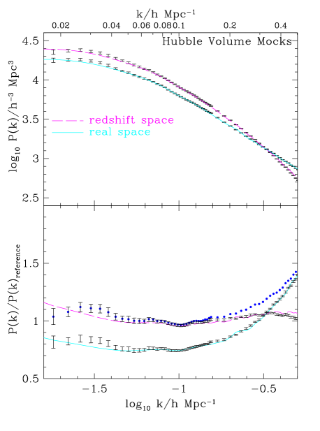
Fig. 11 compares the recovered power spectra with the expected values for three sets of Hubble Volume mocks. As the bias is independent of luminosity for these samples, the power spectrum estimator we use is equivalent to the FKP method. In the first set of mocks, redshift space distortions were eliminated by placing the galaxies at the their real space positions. Here, the power spectrum is isotropic (as in the log-normal mocks) and again we expect, and find, that the recovered power spectrum accurately matches the exact non-linear spectrum from the full Hubble Volume, convolved with the survey window function. The error bars shown on this plot are the errors in the mean power. The rms error for an individual catalogue will be $\sqrt{21}$ times larger, comparable to the error bars in Fig. 10. The second set of points in Fig. 11 are the Hubble Volume mocks constructed using the galaxy redshift space positions. These are compared to the expectation computed by taking the spherically averaged redshift space power spectrum from the full simulation cube and convolving with the window function. We see that over the range of scales plotted, the recovered power agrees well with this expectation. This indicates that ignoring the anisotropy when fitting models will not introduce a significant bias.

In the third set of Hubble Volume mocks, groups and clusters were identified in the redshift space mock catalogues using the same friends-of-friends algorithm and parameters that Eke et al. (2004) used to define the 2PIGG catalogue of 2dFGRS groups and clusters. Each group member was then shifted to the mean group redshift perturbed according to a Gaussian random distribution with width corresponding to the projected group size. This has the effect of collapsing the clusters along the redshift space direction, removing the ‘fingers of god’ and making the small scale clustering much less anisotropic. In the lower panel of Fig. 11 we see that, on large scales, this procedure has no effect on the recovered power. In contrast, on small scales the smoothing effect of the random velocities of galaxies in groups and clusters is removed and the recovered power spectrum has a shape much closer to that of the real space mocks. In Section 8 we will compare the results of analyzing the genuine 2dFGRS data in redshift space with and without this cluster collapsing algorithm.

Figure 12: The data points show the recovered 2dFGRS redshift space galaxy power spectrum for our default set of cuts and weights. The curves show the same realistic model as in Fig. 10, both before and after convolving with the survey window function. In the lower panel, where we have again divided through by an unrealistic reference model with $\Omega_{\rm m}h=0.2$ and $\Omega_{\rm b}=0$, we show both the log-normal estimate of the errors (error bars) and an alternative error estimate based on jack-knife resampling of the 2dFGRS data (shaded region). Note that the window function, shown in Fig. 9, causes the data points to be correlated.

Table 2: The 2dFGRS redshift-space power spectrum. The 3rd column gives the square root of the diagonal elements of the covariance matrix calculated from 1000 realizations of model log-normal density fields. The 4th column gives an alternative empirical estimate of the error based on 20 jack-knife samples. The 5th column gives the value of $P(k)$ convolved with the survey window function for a fiducial linear theory model with $\sigma_{8}^{\rm gal}=0.89$, $h=0.7$, $\Omega_{\rm m}h=0.168$, $\Omega_{\rm b}/\Omega_{\rm m}=0.17$.

$k/{\,h\,\rm Mpc^{-1}}$	$\;\;P_{\rm 2dFGRS}(k)$	$\;\;\sigma_{\rm LN}$	$\;\;\sigma_{\rm jack}$	$P_{\rm ref}(k)$
0.010	43 791.0	19 640.0	15 571.9	22 062.9
0.014	27 021.7	9 569.3	9 538.0	23 280.4
0.018	24 631.7	7 058.4	6 291.8	22 818.3
0.022	26 076.4	6 201.8	5 442.2	21 783.8
0.026	22 163.8	4 603.7	4 441.0	20 477.8
0.030	18 784.6	3 430.5	3 006.7	18 991.5
0.034	17 050.0	2 785.1	2 850.8	17 524.0
0.038	15 233.3	2 283.4	2 521.6	16 153.5
0.042	13 069.6	1 801.0	2 349.1	14 985.6
0.046	13 904.3	1 808.1	2 420.1	14 040.4
0.050	14 085.4	1 703.1	2 110.7	13 183.9
0.054	12 021.6	1 348.5	1 840.4	12 405.9
0.058	11 452.8	1 221.2	1 414.9	11 738.7
0.062	10 829.3	1 099.9	1 283.4	11 114.0
0.066	10 269.5	985.9	1 115.3	10 490.4
0.070	09 477.6	870.1	1 088.4	9 849.1
0.074	09 209.2	822.0	1 107.1	9 205.2
0.078	08 418.5	737.4	807.5	8 571.7
0.082	07 985.5	682.6	697.7	7 967.9
0.086	07 275.4	603.2	737.4	7 426.2
0.090	06 557.0	521.3	607.7	6 916.7
0.094	06 290.2	491.3	658.6	6 462.1
0.099	05 636.1	440.8	421.1	6 070.1
0.103	05 196.2	407.6	385.8	5 748.2
0.107	05 113.0	401.2	406.1	5 479.2
0.111	05 086.4	393.4	536.8	5 242.0
0.115	05 080.4	384.2	515.6	5 028.1
0.119	04 902.5	366.8	482.1	4 820.7
0.123	04 549.7	338.3	298.1	4 606.2
0.127	04 362.7	317.4	244.0	4 392.3
0.131	04 269.7	310.0	241.1	4 181.5
0.135	03 862.7	278.2	220.7	3 969.9
0.139	03 563.6	257.3	209.2	3 767.2
0.143	03 396.6	244.7	205.1	3 577.2
0.147	03 242.2	231.9	202.2	3 401.9
0.151	03 121.7	222.4	162.3	3 248.7
0.155	03 074.0	218.7	175.6	3 112.9
0.169	02 867.9	203.8	239.5	2 728.6
0.185	02 438.2	173.9	170.9	2 362.8

Figure 13: Comparison of the power spectrum estimate from P01 with our current estimates. To compare the amplitude of the new PVP and old FKP estimates, we have scaled the FKP estimate by a factor $\langle b^{-2}\rangle$ (the weighted average value of the bias factor appearing in equation 8). The left hand panel shows each power spectrum estimate divided by a reference power spectrum with parameters $\Omega_{\rm m}h=0.2$ and $\Omega_{\rm b}/\Omega_{\rm m}=0$. In the right hand panel the reference power spectrum has $\Omega_{\rm m}h=0.168,\Omega_{\rm b}/\Omega_{\rm m}=0.17$, and is convolved with the window function of the final or February 2001 data as appropriate. The solid circles with error bars show our standard estimate from the final 2dFGRS catalogue. The triangles show the P01 estimate and the open circles show an estimate using only the pre-February 2001 data but our current calibration and modelling of the survey selection function.

5 Final 2dFGRS results

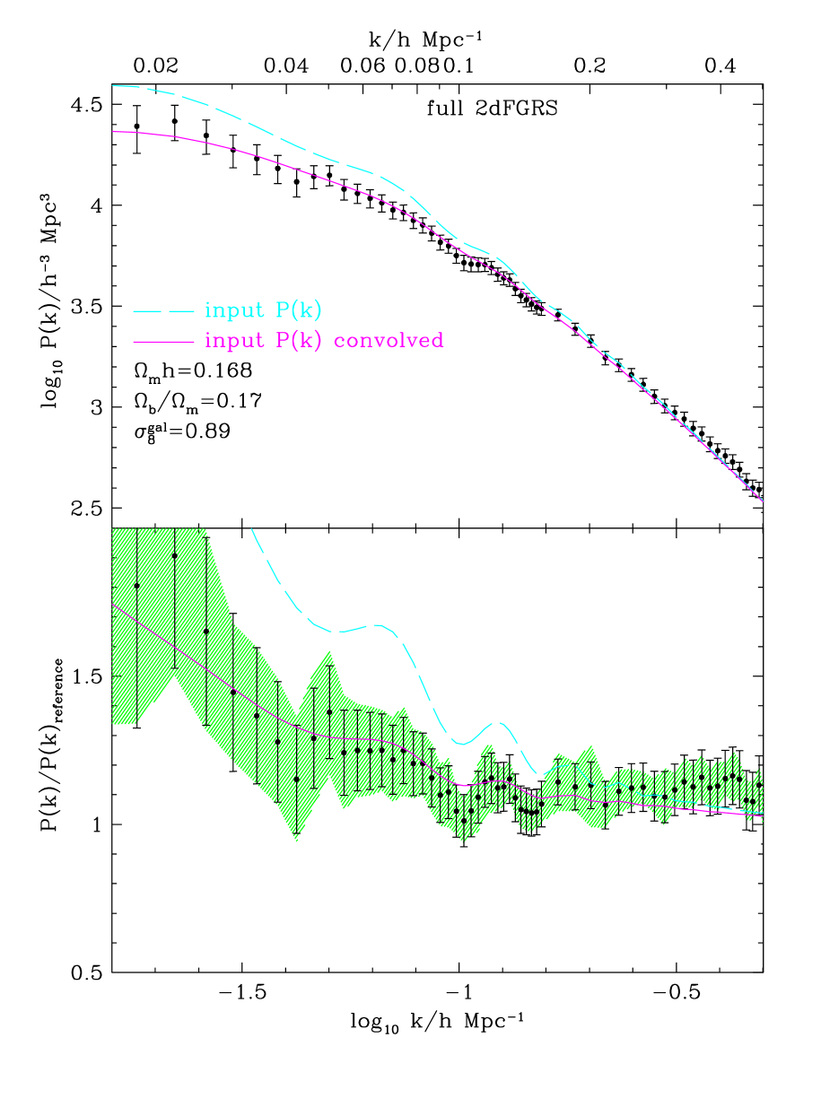
Fig. 12 shows the application of the above machinery to the 2dFGRS data for our default choice of selection cuts, weights and model of the selection function. The error bars on this plot come from a set of log-normal mocks selected, weighted and analysed in the same way. The model power spectrum of these mocks, shown by the curve, has $\Omega_{\rm m}h=0.168$, $\Omega_{\rm b}/\Omega_{\rm m}=0.17$ and $\sigma_{8}^{\rm gal}=0.89$ and closely matches what we recover from the 2dFGRS. The shaded region shows as an alternative a jack-knife estimate of the power spectrum errors. For this, we divided the 2dFGRS data into 20 samples split by RA such that each sample contained the same number of galaxies. We then made twenty estimates of the power, excluding one of the 20 regions in each case. The error bars are $\sqrt{20}$ times the rms dispersion in these estimates. We see that the log-normal and empirical jack-knife error estimate agree remarkably well.

The survey window function causes the power estimates to be correlated and so the plotted error bars alone do not allow one to properly assess the viability of any given model. If the correlations were ignored then the model plotted in Fig. 12 would have an improbably low value of $\chi^{2}$, whereas when the covariance matrix is used one finds a very reasonable $\chi^{2}/{\rm d.f.}=37/33$ for $k<0.2{\,h\,\rm Mpc^{-1}}$. At $k>0.3{\,h\,\rm Mpc^{-1}}$ the estimated power begins to significantly exceed that of the linear theory model. This is due to non-linearity which we discuss in Section 7. These power spectra and error estimates are tabulated in Table 2 . We show in Section 6 that this power-spectrum estimate is robust with respect to variations in how the dataset is treated and we fit models to these data in Section 8.

5.1 Comparison with Percival et al. (2001)

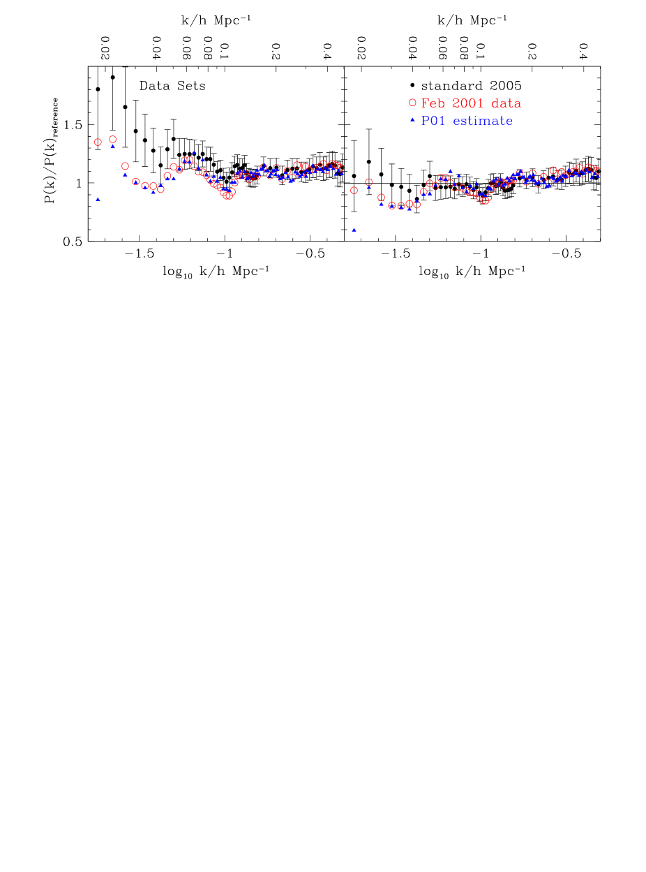
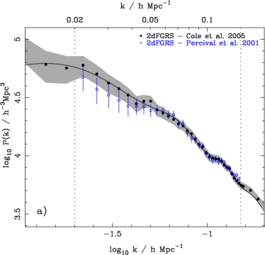
In Fig. 13 we compare our new power spectrum estimate with that from P01. There are significant differences in the shape of the recovered power spectrum on scales larger than $k<0.1{\,h\,\rm Mpc^{-1}}$, but this is largely due to the difference in the window function. In the right hand panel, where this has been factored out, the old and new estimates only begin to differ significantly for $k<0.04{\,h\,\rm Mpc^{-1}}$. The main reason for this difference is sample variance. The estimate shown by the open circles is based on the same dataset as the P01 estimate, but uses the updated calibration, modelling of the selection function and PVP estimator described in this paper. Our current model of the survey selection function differs in many details from that used in P01, but in general these differences make very little difference to the recovered power. The two differences that cause a non-negligible change are the improvement in photometric calibration and the empirical fitted model of the redshift distribution. The perturbation these changes cause are small, restricted to $k<0.04{\,h\,\rm Mpc^{-1}}$ and largely cancel one another out. For the case of the final data set this is discussed in Sections 6.1 and 6.6 and shown in Figs 17d and n.

Figure 14: The various lines show recovered power spectra from 2dFGRS galaxies split into different bins of absolute magnitude (in redshift space – top panel and cluster-collapsed – bottom panel). The power spectra have been divided by a reference model with $\Omega_{\rm m}h=0.168$ and $\Omega_{\rm b}/\Omega_{\rm m}=0.17$, convolved with the window function corresponding to each data cut. We have illustrated statistical errors estimated from log-normal mocks by showing the $\pm 1\sigma$ range for two of the samples by the corresponding shaded regions.

5.2 Dependence on luminosity

The power spectrum we measure comes from combining galaxies of different types, whose clustering properties may be different. We now complete the presentation of the basic results from the survey by dissecting the power spectrum according to galaxy luminosity and colour.

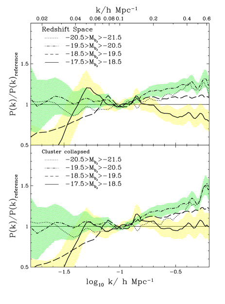
Fig. 14 shows the power spectrum estimated as described in Section 4.1, but for galaxies in fixed bins of absolute magnitude. Because the 2dFGRS catalogue is limited in apparent magnitude, each of these power spectrum measurements will have a different window function; however, we can consider the effect of the window on each power spectrum approximately by dividing the recovered $P(k)$ by the appropriately convolved version of a CDM model that fits the large-scale combined $P(k)$. The power spectra have been renormalized to a common large-scale ($0.02<k<0.08{\,h\,\rm Mpc^{-1}}$) amplitude.

The luminosity-dependent spectra show differences at large and small scales. The variations at $k\mathrel{\lower 2.58334pt\hbox{$\buildrel{\textstyle<}\over{\scriptstyle\sim}$}}0.1{\,h\,\rm Mpc^{-1}}$ are cosmic variance: the different redshift distributions corresponding to different luminosity slices implies that the samples are close to independent. Using the separate covariance matrices for these samples, a $\chi^{2}$ comparison shows that the large-scale variations are as expected. The differences at high $k$, however, reflect genuine differences in the non-linear clustering and/or pairwise velocity dispersions as a function of luminosity. We discuss below in Section 7 how these systematic differences affect our ability to extract cosmological information from the 2dFGRS.

Figure 15: Power spectrum for matched red and blue galaxy subsamples. The symbols and error bars in the upper panel show our estimates with errors derived from the log-normal mocks. For reference, the solid curves show the linear power spectrum used for the log-normal mocks, which has $\Omega_{\rm m}h=0.168$ and $\Omega_{\rm b}/\Omega_{\rm m}=0.17$. In each case, the model power spectra are normalized according to the bias parameters defined in equations (10) and (11) and convolved with the window function of the sample. The lower panel shows the relative bias, the square root of the ratio of these power spectra. The error bars, determined from our mock catalogues, take account of the correlation induced by the fact the red and blue subsamples sample the same volume. The horizontal line in the lower panel shows the expectation for scale independent bias given by the ratio of $b(L_{*})$ for the adopted red and blue bias factors from equations (10) and (11). The solid curves show the ratio that would result if the red and blue galaxies had power spectra that were well described by linear theory models whose values of $\Omega_{\rm m}h$ differed by $0.01$, $0.02$ or $0.03$ from top to bottom on large scales.

5.3 Dependence on colour

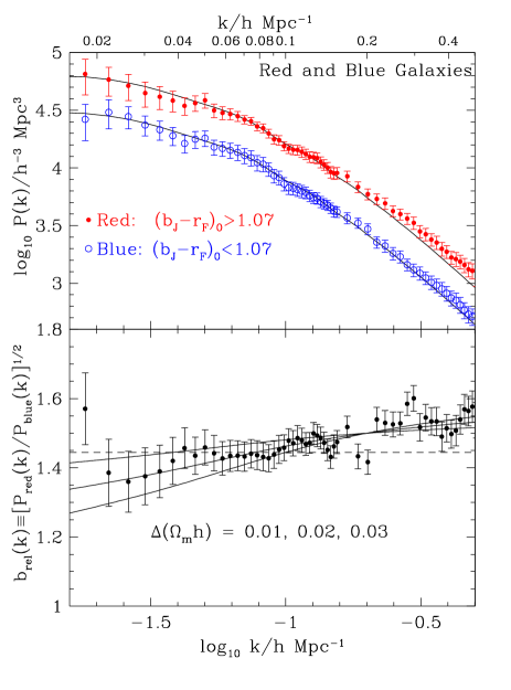
In Fig. 15, we show estimates of the galaxy power spectrum for the two samples defined by splitting the catalogue at a rest frame colour of $({\rm b_{J}}-r_{\rm\scriptscriptstyle F})_{z=0}=1.07$. As the redshift distribution of the blue sample is more extended than that of the red, the optimal PVP weighting for the blue sample weights the volume at high redshift more strongly. Since we wish to compare the shapes of the red and blue power spectra it would be preferable if they sampled the same volume. Hence, when analyzing the blue sample, we have chosen to apply an additional redshift dependent weight, so as to force the mean weight per unit redshift to be the same for both samples. The estimates were made using the PVP estimator and the bias parameters defined in equations (10) and (11). However, to illustrate that at fixed luminosity the red galaxies are more clustered than the blue galaxies we have multiplied each estimate by their respective values of $b(L_{*})^{2}$, where $L_{*}$ is the characteristic luminosity of the full galaxy sample. To first order, we see that the two power spectra have very similar shapes, with both becoming more clustered than the linear theory model on small scales.

Figure 16: The redshift-space power spectrum calculated in this paper (solid circles with 1-$\sigma$ errors shown by the shaded region) compared with other measurements of the 2dFGRS power spectrum shape by a) Percival et al. (2001), b) Percival (2005), and c) Tegmark et al. (2002). For the data with window functions, the effect of the window has been approximately corrected by multiplying by the net effect of the window on a model power spectrum with $\Omega_{\rm m}h=0.168$, $\Omega_{\rm b}/\Omega_{\rm m}=0.0$, $h=0.72$ & $n_{\rm s}=1$. A zero-baryon model was chosen in order to avoid adding features into the power spectrum. All of the data are renormalized to match the new measurements. Panel d) shows the uncorrelated SDSS real space $P(k)$ estimate of Tegmark et al. (2004), calculated using their ‘modelling method’ with no FOG compression (their Table 3). These data have been corrected for the SDSS window as described above for the 2dFGRS data. The solid line shows a model linear power spectrum with $\Omega_{\rm m}h=0.168$, $\Omega_{\rm b}/\Omega_{\rm m}=0.17$, $h=0.72$, $n_{\rm s}=1$ and normalization matched to the 2dFGRS power spectrum.

The lower panel shows the relative bias, $b_{\rm rel}(k)\equiv\sqrt{P_{\rm red}(k)/P_{\rm blue}(k)}$, as a function of scale. On large scales, this relative bias is consistent with a constant and is, by construction, close to the value given by the ratio of the adopted bias parameters of equations (10) and (11) shown by the horizontal dashed line. In fact, for $k<0.12{\,h\,\rm Mpc^{-1}}$, fitting a constant bias using the full covariance matrix produces a fit with $\chi^{2}=25.5$ for 25 degrees of freedom. We note that this value of the bias, $b_{\rm red}/b_{\rm blue}=1.44$ is in very good agreement with the $b_{\rm passive}/b_{\rm active}=1.45\pm 0.14$ found in section 3.3 of Madgwick et al. (2003), when analysing the correlation function of spectrally classified 2dFGRS galaxies. The value also agrees well with that found in the halo model analysis of red and blue 2dFGRS galaxies by Collister & Lahav (2005). At smaller scales, there is an increasingly significant deviation, with the red galaxies being more clustered than the blue (in agreement with Madgwick et al., 2003). Also shown in the lower panel are curves indicating the relative bias that would result if the red and blue power spectra were well fitted by linear theory models whose values of $\Omega_{\rm m}h$ differed by $0.01$, $0.02$ or $0.03$. From this we see that a simple fit of linear theory to the red and blue samples would yield values of $\Omega_{\rm m}h$ that differ by $\Delta\Omega_{\rm m}h\simeq 0.015$. This small difference is comparable to the statistical uncertainty. In any case, in Section 7 we discuss systematic nonlinear corrections to the power, and show how a robust measurement of $\Omega_{\rm m}h$ can be achieved even in the presence of small distortions of the spectrum.

5.4 Comparison with other power spectra

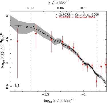
In Fig. 16, we compare the power spectrum measured in this paper with previous estimates of the shape of the power spectrum on large-scales measured from the 2dFGRS and SDSS. In addition to the data of Percival et al. (2001), with which we compared in detail in Section 5.1, we additionally plot the data of Percival (2005) who extracted the real-space power spectrum from the 2dFGRS. In that work, Markov-chain Monte-Carlo mapping of the likelihood surface was used to deconvolve the power spectrum from a Spherical Harmonics decomposition presented in Percival et al. (2004b). Because of the method used, a cut-down version of the final 2dFGRS catalogue was analysed with a radial selection function that was independent of angular position. Consequently, the volume analysed is smaller, and this method provides weaker constraints on the power spectrum shape. However, we see from Fig. 16b that the general shape of the recovered power spectrum is very similar over $0.02<k<0.15{\,h\,\rm Mpc^{-1}}$, the range of scales probed in Percival (2004b).

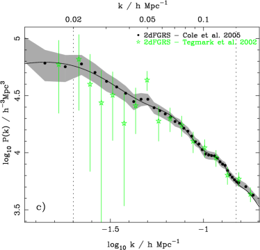
In Fig. 16c we plot the power spectrum measured by Tegmark et al. (2002) from the 2dFGRS 100k data release. Because of the weighting scheme they used, these data are expected to be tilted relative to the true power spectrum because of luminosity-dependent bias. The plot shows evidence for such a bias and the Tegmark et al. (2002) data have a lower amplitude on large scales than any of the other 2dFGRS $P(k)$ measurements. Given the small sample analysed, these data provide a far weaker constraint on the power spectrum shape than our current analysis.

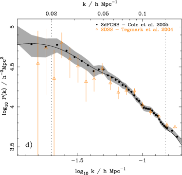
In addition to the 2dFGRS power spectrum measurements described above, we also plot in Fig. 16d the recent estimate from the SDSS by Tegmark et al. (2004). This analysis differed from the analysis of the 2dFGRS by Tegmark et al. (2002) by including a crude correction for luminosity-dependent bias, which corrects for an amplitude offset for each data point, but does not allow for the changing survey volume (Percival et al. 2004a). The SDSS work quotes a somewhat larger value of $\Omega_{\rm m}h$ than that found here: $0.213\pm 0.023$, which is formally a $1.6-\sigma$ deviation. However, this SDSS figure assumes a known baryon fraction, which makes the error on $\Omega_{\rm m}h$ unrealistically low. As can be seen from Fig. 16d, the basic shapes of the 2dFGRS and SDSS galaxy power spectra in fact agree remarkably well.

We have chosen not to compare with galaxy power spectrum estimates obtained from surveys prior to the 2dFGRS, or calculated by deprojecting 2D surveys because the 2dFGRS and SDSS data offer a significant improvement over these data. However, we do note that the general shape of our estimate of the power spectrum is very similar to that obtained in such studies (e.g. Efstathiou & Moody 2001; Padilla & Baugh 2003; Ballinger, Heavens & Taylor 1995; Tadros et al. 1999).

6 Tests of systematics

Given the cosmological significance of the 2dFGRS power spectrum estimates, it is important to be confident that the results presented in the previous Section are robust, and not sensitive to particular assumptions made in the analysis. This Section presents a comprehensive investigation into potential sources of systematic error in the final result.

Our default set of assumptions in modelling and analyzing the 2dFGRS data are:

1. Our standard choice for the photometric calibration of the catalogue is essentially that of the final data release (Colless et al., 2003) but with small shifts of $-0.0125$ and $0.022$ mag. applied to the NGP and SGP respectively to bring their estimated luminosity functions into precise agreement.

2. We combine data from the NGP and SGP strips and also the RAN fields.

3. We model the galaxy population by a single Schechter luminosity function and $k+e$ correction as described in Section 3 and shown in Fig. 5. Magnitude measurement errors are then applied using the empirical model of Norberg et al. (2002b see their figure 3f).

4. Incompleteness in the redshift survey is modelled in the mock catalogues using a combination of the mean completeness in each sector $R(\theta)$ (Fig. 3) and its dependence on apparent magnitude as parameterized by $\mu(\theta)$ (Fig. 4; see Colless et al. 2001 Section 8 and appendix A of Norberg et al. 2002b for details).

5. We discard data from sectors with redshift completeness $R(\theta)<0.1$.

6. We impose a maximum redshift of $z_{\rm max}=0.3$ .

7. We use the PVP estimator with the bias parameter given by equation 9.

8. We use angular weights that attempt to correct for missed close pairs due to fibre collisions and positioning constraints. Their construction is explained in Section 6.3.

9. We use the radial weighting given by equation (12) with $J_{3}=400h^{-3}$Mpc³.

Figure 17: Test power spectra calculated for different data cuts and assumptions. The data are divided by a reference power spectrum. In the left hand column, the reference power spectrum has parameters $\Omega_{\rm m}h=0.2$ and $\Omega_{\rm b}/\Omega_{\rm m}=0$. In the right hand column, the reference power spectrum has $\Omega_{\rm m}h=0.168,\Omega_{\rm b}/\Omega_{\rm m}=0.17$ (as used for the log-normal mock catalogues), and is convolved with the correct window function (which varies with data cuts and weighting scheme). The top row shows the power spectrum estimate and associated statistical errors resulting from our standard choices of data cuts and weighting. Subsequent rows give results for different tests, as described in Section 6.

Figure 18: continued

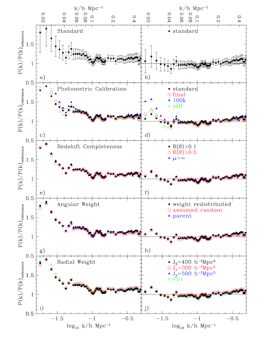
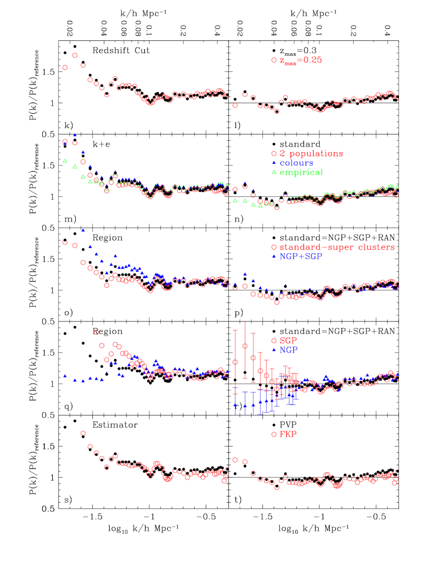
In Fig. 17, the left hand panels show the ratio of estimated power spectra to an (unrealistic) reference model power spectrum with $\Omega_{\rm m}h=0.2$ and $\Omega_{\rm b}/\Omega_{\rm m}=0$. These panels allow one to see the effect of our modelling assumptions on the shape and amplitude of the recovered power spectrum. However, part of this variation will be due to how the survey window function changes when we modify the weighting or selection cuts. Thus, the right hand panels show the same power spectra, but divided instead by the realistic model with $\Omega_{\rm m}h=0.168$ and $\Omega_{\rm b}/\Omega_{\rm m}=0.17$ that was used for the log-normal mocks, but now taking into account the correct window function for each dataset. Unless stated otherwise, no adjustments are made to the normalization of the power spectrum estimates.

The top panels of Fig. 17 show the estimated power spectrum for the full 2dFGRS for the standard choices listed above. The error bars are those we estimate from the log-normal mock catalogues. In the subsequent panels of Fig. 17, we show the effects of varying these assumptions.

6.1 Photometric calibration

Over the years the earlier calibrations of the APM photographic plates have been the source of much debate (e.g. Metcalfe, Fong & Shanks, 1995; Busswell et al., 2004). Thus it is important to try and quantify at what level uncertainties in the photometry have an impact on our ability to measure the galaxy power spectrum.

Results of four different calibrations are shown in Figs 17c and d. As described in Section 2.1, our standard choice (standard) differs from the final 2dFGRS calibration (final) by the small offsets that we apply to the NGP and SGP regions so as to bring their luminosity functions into good agreement. We see that these offsets cause very little change in the recovered power spectrum. We also show results for the older calibration from the preliminary 100k data release (100k) (Colless et al., 2001). Here, the systematic shift in the recovered power spectrum is somewhat larger, but as the size of the error bars in the upper panels show the shift is never larger than the statistical error. If we had used this calibration, then the maximum likelihood value of $\Omega_{\rm m}h$ inferred in Section 8 would have been reduced by $0.01$ and the baryon fraction $\Omega_{\rm b}/\Omega_{\rm m}$ increased by $0.04$. These shifts are almost equal to the $1-\sigma$ statistical errors in these quantities.

For the last calibration model shown in Figs 17c and d, we take a novel approach and first calibrate each photographic plate without the use of external photometric data. The magnitudes in the final released catalogue, ${\rm b_{J}}^{\rm final}$ and magnitudes, ${\rm b_{J}}^{\rm self}$, resulting from this self-calibration are assumed to be related by a quasilinear relation

$${\rm b_{J}}^{\rm self}=a_{\rm self}\,{\rm b_{J}}^{\rm final}+b_{\rm self}.$$ (21)

The calibration coefficients $a_{\rm self}$ and $b_{\rm self}$ are allowed to vary from plate to plate. To set the values of these calibration coefficients two constraints are applied. First, on each plate we assume that the galaxy luminosity function can be represented by a Schechter function with faint-end slope $\alpha=-1.2$ and make a maximum likelihood estimate of $M_{*}$. The value of $M_{*}$ is sensitive to the difference in ${\rm b_{J}}^{\rm self}$ and ${\rm b_{J}}^{\rm final}$ at around ${\rm b_{J}}=17.5$ and the number of galaxies on each plate is such that the typical random error on $M_{*}$ is $0.03$ magnitudes. Second, we compare the number of galaxies, $N(z>0.25)$, with redshifts greater than $z=0.25$ with the number we expect, $N_{\rm model}(z>0.25)$, based on our standard model of the survey selection function. The value of $N_{\rm model}(z>0.25)$ depends sensitively on the survey magnitude limit and so constrains the difference in ${\rm b_{J}}^{\rm self}$ and ${\rm b_{J}}^{\rm final}$ at ${\rm b_{J}}\simeq 19.5$. By demanding that on each plate both $N(z>0.25)=N_{\rm model}(z>0.25)$ and $M_{*}-5\log h\equiv-19.73$, we determine $a_{\rm self}$ and $b_{\rm self}$. Note that this method of calibrating the catalogue is extreme. It ignores the information available in the plate overlaps and ignores the CCD calibrating data (apart from setting the overall arbitrary zero point of $M_{*}-5\log h=-19.73$). Nevertheless, we see that this (self) and the default (standard) calibration results in only a very small shift in the recovered power spectrum. The corresponding shifts in the inferred cosmological model parameters $\Omega_{\rm m}h$ and baryon fraction $\Omega_{\rm b}/\Omega_{\rm m}$ are $-0.006$ and $0.02$ respectively. These shifts are small compared to the corresponding statistical errors.

We conclude from these comparisons that the final 2dFGRS photometric calibration is more accurate than the preliminary 100k calibration and the residual systematic uncertainties are at a level that they have negligible impact on the accuracy of the recovered galaxy power spectrum.

6.2 Redshift incompleteness

In Figs 17e and f, we investigate the effect of varying the treatment of incompleteness in the redshift survey. As described above, our default choice is to keep all sectors of the survey with a completeness $R(\theta)>0.1$ and use the completeness maps shown in Fig. 3 and Fig. 4 to reproduce this in the random catalogues. In Figs 17e and f, we show the effect of using the much more stringent cut $R(\theta)>0.5$ and so removing the tail of low completeness sectors that are visible in Fig. 3. These are mainly around the edges of the survey where constraints on observing time meant that overlapping fields were never observed. This has a very small, but measurable effect on the $P(k)$ shown in Fig. 17e, but once the effect of the changed window function is accounted for, no perceptible difference remains in Fig. 17f.

Also shown in these panels is the effect of ignoring the apparent magnitude dependence of the incompleteness by setting $\mu=\infty$ when constructing our random catalogues. Again, there is negligible effect, clearly demonstrating that the accuracy of the 2dFGRS galaxy power spectrum is not affected by uncertainty in the incompleteness.

6.3 Angular weight

In Figs 17g and h, we show the effect of varying the angular weights which compensate for redshifts that are missed due to fibre collisions. Our default choice of the angular weights, $w^{\rm A}$, that attempt to correct for missing close pairs, are defined by a multi-step process. We assign unit weight to all objects in the 2dFGRS parent catalogue, then loop over the subset that lack measured redshifts and redistribute their weight to their 10 nearest neighbours with redshifts. The angular weights, $w^{A}$, are then defined by multiplying these weights by $R(\theta)$ and explicitly normalizing them to have an overall mean of unity. The inclusion of the $R(\theta)$ factor means that the overall weight assigned to a given sector is proportional to the number of galaxies in that sector with measured redshifts, rather than to the number in the parent catalogue. The estimate labelled ‘assumed random’ instead has $w^{A}\equiv 1$ and so no correction is made for missing close pairs other than their contribution to the overall completeness of a given sector, i.e.  within a sector the missing galaxies are assumed to be a random subset. We see that, on the scale of interest, correcting for the missing close pairs has a negligible effect.

For the estimate labelled ‘parent’ we omit the factor $R(\theta)$ in the construction of the angular weights for the main NGP and SGP strips. This has the effect of up-weighting regions with low completeness so that each sector has a weight proportional to the number of galaxies in the parent catalogue. Hence the angular dependence of the window function that is due to varying redshift incompleteness is removed. Figs 17g and h show that even for this very different weighting, the change in the recovered power spectrum is extremely small.

6.4 Radial weight

In Figs 17i and j, we investigate the effect of varying the radial weighting function. We show the result of using equation 12 with $J_{3}=300$, $400$ and $500h^{-3}$Mpc³. The choice of weighting alters the effective window function and so there is some variation in the left hand panel on the very largest scales, but in the right hand panel, where this is factored out, there is very little variation in the recovered power. For each of these values of $J_{3}$, we generated a set of 1000 log-normal mocks and compared the statistical error in the recovered power, measured from the rms scatter in the individual estimates. This exercise explicitly verified that the value $J_{3}\simeq 400\,h^{-3}$Mpc³, that we adopt as a default, is close to optimal in terms of giving a minimal variance estimate of the power.

The weighting function, equation 12, depends not only on redshift, but also on angular position through the angular dependence of the quantity ${{\bar{n}}_{\rm L}^{\rm g}}$. That is, it takes account of the variation in the expected galaxy number density due to angular variation of redshift incompleteness and survey magnitude limit. The estimates labelled ‘P01’ use instead a purely redshift dependent weight of

$$w=(1.0+100/[1+(z/0.12)^{3}]^{2})^{-1}$$ (22)

as was done in Percival et al. (2001). On average, this is close to our $J_{3}=400h^{-3}$Mpc³ weighting. It slightly modifies the window function, but once this is factored out we see, in Fig. 17j, that there is little effect on the recovered power.

6.5 Redshift limit

In Figs 17k and l, we reduce the redshift limit from $0.3$ to $0.25$. This alters the window function and so has an effect on the power plotted in the left hand panel, but in the right hand panel, where this is corrected for, the variation is minimal. The accurate agreement here is reassuring and indicates there are no problems in pushing the survey and the model of its selection function to the full volume that it probes.

6.6 Luminosity function and evolution

In Figs 17m and n, we investigate the uncertainty in the recovered power induced by the uncertainty involved in the radial selection function of the survey. Our default determination of the 2dFGRS selection function involves modelling the galaxy luminosity function as a single Schechter luminosity function and the evolution by a single $k+e$ correction (magnitude measurement errors are also included). These are derived empirically by the maximum likelihood method presented in Section 3. This ‘standard’ model is compared with the result of using a ‘2 population’ model with individual luminosity functions and $k+e$ corrections for the red and blue galaxy populations. Again, the luminosity functions and $k+e$ corrections used are the empirically determined ones presented in Section 3. We see that adding these extra degrees of freedom to the description of the galaxy population has a negligible effect on the recovered power.

As a separate test, we show the results (labelled ‘colours’) of a single population model in which the mean $k+e$ correction has been determined using Bruzual & Charlot (1993) stellar population models matched to the galaxy colours as was done in Norberg et al. (2002b). This model again produces highly consistent results, which is perhaps not surprising given that its $k+e$ correction, shown in Fig. 5, is quite similar to the one found by the maximum likelihood method.

The three radial selection function models discussed above produce consistent results, but all make common assumptions such as Schechter function forms for the luminosity functions and smooth $k+e$ corrections. To demonstrate that these assumptions are not artificially distorting our estimate of the power, we present results for an alternative empirical model of the redshift distribution. For this, we compare the observed redshift distribution averaged over the whole survey with that of our standard model. The two redshift distributions are shown in the top panel of Fig. 6. We then resample our default random catalogues so that the redshift distribution of the remaining galaxies exactly matches that of the data. In this process we also correspondingly modify the tabulated galaxy number densities in the random catalogue so that our power spectrum estimator remains correctly normalized. Note that this procedure is not equivalent to simply generating a random catalogue by shuffling the data redshifts as we retain the modulation of the redshift distribution caused by the varying survey magnitude limit that was built into the standard random catalogue.

Fig. 17n shows that the only effect of adopting this empirical redshift distribution is, unsurprisingly a reduction of the power on the very largest scales and that even here the shift is not large compared to the statistical errors. Adopting this estimate rather than our standard one only shifts our estimates of the cosmological parameters $\Omega_{\rm m}h$ and $\Omega_{\rm b}/\Omega_{\rm m}$ by $+0.006$ and $-0.03$ respectively. These shifts, which are smaller than the $1\sigma$ statistical errors, should be considered extreme, as adopting an empirical redshift distribution will undoubtedly lead to the removal of some genuine large scale radial density fluctuations.

6.7 Region

In Figs 17o,p,q and r, we show the effect of excluding various regions from our analysis. The effect of excluding the random fields is very modest. In particular, we note that the oscillatory features in the estimated power spectra around $k\approx 0.15{\,h^{-1}\,\rm Mpc}$ are present both with and without the random fields and that once the effects of the very different window functions (see Fig. 9) have been compensated for, Fig. 17p, the power spectra agree very accurately. This clearly demonstrates that these features are not related to the presence or absence of a secondary peak in the window function. Also shown in Figs 17o and p is the effect of excluding from our data the two superclusters identified by Baugh et al. (2004) and Croton et al. (2004) and mapped using the Wiener filtering technique by Erdogdu et al. (2004). The northern supercluster is the heart of the structure that has also become known as the Sloan great wall (Gott et al., 2005). Here we have simply excised these superclusters by cutting out regions of 9x9 degrees and $\Delta z=0.1$ centred on the superclusters. These superclusters are known to perturb higher order clustering statistics significantly (Croton et al., 2004), but we see that their removal causes a negligible reduction in the large-scale power. Using this dataset only shifts our estimates of the cosmological parameters $\Omega_{\rm m}h$ and $\Omega_{\rm b}/\Omega_{\rm m}$ by $+0.008$ and $-0.026$ respectively. These shifts are much smaller than the $1-\sigma$ statistical errors. Also, as genuine structure is being removed one expects the large-scale power to be suppressed. Clearly these superclusters do not significantly perturb our estimated power spectrum.

Excluding either the NGP or SGP strips has a large effect on the window function and this is partly responsible for the changes in the recovered power seen in Fig. 17q. But in this case cosmic variance is also important and so, even when we compensate for the window, as is done in Fig. 17r, we do not expect perfect agreement between these estimates; for independent samples, we would expect differences comparable to the statistical errors. The errors from our log-normal mocks shown on the independent NGP and SGP estimates indicate that only on the very largest scales, where the data points are highly correlated, do the estimates differ by more than $1\sigma$. If the likelihood analysis described in Section 8 is applied separately to these two samples we find $\Omega_{\rm m}h=0.168\pm 0.035$, $\Omega_{\rm b}/\Omega_{\rm m}=0.163\pm 0.075$ for the SGP and $\Omega_{\rm m}h=0.205\pm 0.037$, $\Omega_{\rm b}/\Omega_{\rm m}=0.116\pm 0.072$ for the NGP, which are entirely consistent within their statistical errors.

6.8 Estimator

In Figs 17s and t, we compare the result of using the FKP rather than the PVP estimator. We have adjusted the normalization of the FKP estimate by a factor $\langle b^{-2}\rangle$ to account for the normalization difference in the definition of the two estimators. If galaxies have a luminosity dependent bias, then the FKP estimator is biased, with the result that one recovers a power spectrum convolved with an effective window function that is slightly different to the one assumed (PVP). Provided the model of luminosity dependent bias is correct, then the PVP estimator removes this bias. The two recovered power spectra shown in Fig. 17t differ only slightly in shape indicating that the bias resulting from using the FKP estimator, as was done in P01, is small. Furthermore, even if our model of bias dependence on luminosity and colour is not highly accurate, the effect on the recovered power spectrum will be significantly smaller than the difference between the FKP and PVP estimates and so entirely negligible.

6.9 Summary

In conclusion, we have not identified any systematic effects at a level that is significant compared to the statistical errors. We return to this point in Section 8, where we show explicitly how various systematic uncertainties affect the likelihood surfaces that quantify our constraints on cosmological parameters.

7 Non-linearity and scale-dependent bias

The previous Section has demonstrated that we can measure the spherically-averaged redshift-space power spectrum of the 2dFGRS in a robust fashion. We now have to consider in detail the critical issue of how the galaxy measurements relate to the power spectrum of the underlying density field.

The conventional approach is to assume that, on large enough scales, linear theory provides an adequate description of the shape of the galaxy power spectrum. In reality, this agreement can never be perfect, and we need a model for the differences between the galaxy power spectrum and linear theory. In this Section, we pursue a number of approaches for estimating such corrections; detailed simulations, analytical models, and an empirical hybrid approach are all considered.

7.1 Simulated galaxy catalogues

Figure 19: The power spectrum of the mass and galaxies in the Hubble Volume simulation cube. The solid curve in the upper panel shows the input linear theory power spectrum. The dotted and dashed curves show the power spectrum for the galaxies in real and redshift space respectively. In the lower panel, using the same line types, we show these galaxy power spectra divided by the linear theory power spectrum, scaled by the square of expected bias factor. The solid curve shows the ratio of the mass to linear theory power spectra.

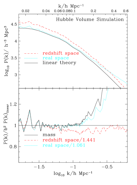
We start by considering the power spectrum of the Hubble Volume galaxies. Fig. 19 shows results from the full Hubble Volume, both in real and redshift space. Here, we use all $10^{9}$ particles in the simulation cube weighted by the probability of each particle being selected as a galaxy. On large scales ($k\mathrel{\lower 2.58334pt\hbox{$\buildrel{\textstyle<}\over{\scriptstyle\sim}$}}0.1\,{\,h^{-1}\,\rm Mpc}$) both the real-space and redshift-space galaxy power spectra are related to linear theory by a simple scale independent constant. The large scale linear bias factor for the galaxies in real space is $b=1.03$. On these large scales the redshift-space power is boosted by the Kaiser (1987) factor $b^{2}(1+2/3\,\beta+1/5\,\beta^{2})$; here $\beta=\Omega_{\rm m}^{0.6}/b=0.471$, so the expected boost factor is 1.441, in excellent agreement with the simulation results.

In real space, both the mass and galaxy power spectra begin to exceed the linear theory prediction significantly for $k\mathrel{\lower 2.58334pt\hbox{$\buildrel{\textstyle>}\over{\scriptstyle\sim}$}}0.12{\,h\,\rm Mpc^{-1}}$. In redshift space, the smearing effect of the random galaxy velocities reduces the small scale power with the result that deviations from linear theory are greatly reduced. This cancellation of the distortions caused by non-linearity, bias and mapping to redshift space was used in P01 to motivate fitting the 2dFGRS with linear theory for $k<0.15{\,h\,\rm Mpc^{-1}}$. The Hubble Volume results presented here reinforce this argument, although there is a suggestion that the redshift-space power underestimates linear theory by up to 10% on small scales.

The Hubble Volume simulations are realistic in some respects, but they do not treat the relation between mass and light in a particularly physical way. According to current understanding, the location of galaxies within the dark matter is determined largely by the dark-matter halos and their merger history. Full semi-analytic models of galaxy formation follow halo merger trees within a numerical simulation, and can yield impressively realistic results. An important landmark for this kind of work was the paper by Benson et al. (2000), who showed how a semi-analytic model could naturally yield a correlation function that is close to a single power law over $1000\mathrel{\lower 2.58334pt\hbox{$\buildrel{\textstyle>}\over{\scriptstyle\sim}$}}\xi\mathrel{\lower 2.58334pt\hbox{$\buildrel{\textstyle>}\over{\scriptstyle\sim}$}}1$, even though the mass correlations show a marked curvature over this range. We have used the most recent version of this code to predict the galaxy power spectra, and their ratio to linear theory. This is shown in Fig. 20, for a model close to our final preferred cosmology: $\Omega_{\rm m}=0.25$, $\Omega_{\rm b}=0.045$, $h=0.73$ and $\sigma_{8}=0.9$. The simulation volume has a side of $1000{\,h^{-1}\,\rm Mpc}$ and $10^{9}$ simulation particles. One advantage of this more detailed simulation is that the predicted colour distribution is bimodal, and so we are able to identify red and blue subsets in the same way as for the real data.

These results paint a similar picture to what was seen in the Hubble Volume, despite the very different treatment of bias. On intermediate scales, there is a tendency for galaxy power to lie below linear theory. In real space, this trend reverses around $k=0.1{\,h\,\rm Mpc^{-1}}$, and galaxy power exceeds linear theory for $k\ga 0.2{\,h\,\rm Mpc^{-1}}$. A small-scale increase is also seen in redshift space, but redshift-space smearing naturally means that the effect is reduced.

It will be convenient to consider a fitting formula for the distortion seen in this simulation, and the following simple form works well:

$$P_{\rm gal}={1+Qk^{2}\over 1+Ak}\;P_{\rm lin}.$$ (23)

The required parameters to fit the ‘all galaxy’ data, shown by the dashed lines in Fig. 20, are $A=1.7$ and $Q=9.6$ (real space) or $A=1.4$ and $Q=4.0$ (redshift space). The critical question is whether this correction is robust, both with respect to variations in the galaxy-formation model and variations in cosmology. It is impractical to address this directly by running a large library of simulations, so we consider an alternative analytic approach.

7.2 The halo model

The success of Benson et al.’s work stimulated the analytic ‘halo model’, which allows one to understand rather simply the differences in shape between the galaxy and mass power spectra (Seljak 2000; Peacock & Smith 2000; Cooray & Sheth 2002). In this approach, the galaxy density field results from a superposition of dark-matter halos, with small-scale clustering arising from neighbours in the same halo.

Using the halo model, it is possible to predict the relation between the galaxy power spectrum and linear theory. This can be done as a function of galaxy type, by an appropriate choice of prescription for the occupation numbers of halos as a function of their mass. In effect, we can give particles in halos a weight that depends on halo mass, as was first considered by Jing, Mo & Börner (1998). A simple but instructive model for this is

$$w(M)=\cases{0\quad&($M<M_{c}$)\cr(M/M_{c})^{\alpha-1}\quad&($M>M_{c}$)\cr}$$ (24)

A model in which mass traces light would have $M_{c}\rightarrow 0$ and $\alpha=1$. In practice, data on group $M/L$ values argues for $\alpha$ substantially less than unity (Peacock & Smith 2000, see also Collister & Lahav 2005). More elaborate occupation models can be considered (e.g. Tinker et al. 2005; Zheng et al. 2005) and have previously been applied to model 2dFGRS galaxy clustering (Van den Bosch, Yang & Mo, 2003; Magliocchetti & Porciani, 2003), but this simple model will suffice for the present purpose: we are trying to estimate a small correction in any case, and are largely interested in how it may vary with cosmology.

Figure 20: Predictions for how the redshift-space power spectrum of galaxies may be expected to deviate from linear theory. A model with $\Omega_{\rm m}=0.25$, $\Omega_{\rm b}=0.045$, $h=0.73$ and $\sigma_{8}=0.9$ is assumed. The predictions of semi-analytic modelling are shown as points: filled circles denote red galaxies; open circles denote blue galaxies; stars denote all galaxies (to $M_{{\rm b_{J}}}<-19$). The dashed line shows the fitting formula described in the text. The solid lines show the predictions made using the halo model for red (upper), blue (lower) and all (intermediate) galaxies. The occupation parameters are adjusted so as to fit the real-space correlation functions from Madgwick et al. (2003). We attempt to make the calculation more robust by modelling the conversion between real and redshift space using the Ballinger et al. (1996) prescription. We use observed values of $\beta=0.49$ and $\beta=0.48$ and large-separation effective pairwise dispersions of $280{\,\rm km\,s^{-1}}$ and $410{\,\rm km\,s^{-1}}$ for late and early types respectively from Madgwick et al. (2003) and Hawkins et al. (2003)

Figure 21: A more extensive set of predictions for the deviation of the galaxy power spectrum from linear theory, using the halo model as in Fig. 20. We retain $\Omega_{\rm b}=0.045$ and $h=0.73$, but vary $\Omega_{\rm m}$ between 0.17 and 0.35. The normalization is chosen to scale as $\sigma_{8}=0.9(0.25/\Omega_{\rm m})^{0.6}$, as expected for a normalization to redshift-space distortions or cluster abundance. The plotted ratio is a weakly declining function of $\Omega_{\rm m}$ (i.e. the lowest $\Omega_{\rm m}$ gives the strongest kick-up at high $k$).

The translation of the halo model into redshift space has been discussed by White (2001), Seljak (2001) and Cooray (2004). In the halo model, one thinks of the real-space power spectrum as being a combination of two parts:

$$P_{r}=P_{\rm 2-halo}+P_{\rm 1-halo},$$ (25)

representing the effect of correlated halo centres (the first term), plus power owing to halo discreteness and internal structure of a single halo (the second term). In redshift space, we expect the first term to undergo Kaiser (1987) distortions, so that it gains a factor $(1+\beta\mu^{2})^{2}$, where $\mu$ is the cosine of the angle between the wavevector and the line of sight. Having shifted the halo centres to redshift space, the effect of virialized velocities is to damp the total power for modes along the line of sight:

$$P_{s}=\left((1+\beta\mu^{2})^{2}P_{\rm 2-halo}+P_{\rm 1-halo}\right)\;D^{2}(\mu k).$$ (26)

For a Gaussian distribution of velocities within a halo, the damping factor is

$$D(x)=\exp\left(-x^{2}/2\sigma_{v}^{2}\right);$$ (27)

here, $\sigma_{v}$ denotes the one-dimensional halo velocity dispersion in units of length (i.e. divided by $H_{0}$). This expression applies for the case where $\beta$ and $\sigma_{v}$ are the same for all halos. Since both vary with mass, the expression must be appropriately averaged over halo mass, as described in the above references.

This completes in outline the method needed to calculate the redshift-space power spectrum. However, we will not use all this apparatus: the halo model was not designed to work at the precision of interest here, and we will therefore use it only in a differential way which should minimize systematics in the modelling. The power ratio of interest can be expressed as

$${P_{\rm gal}^{s}\over P_{\rm lin}}={P_{\rm gal}^{r}\over P_{\rm nl}}\times{P_{\rm nl}\over P_{\rm lin}}\times{P_{\rm gal}^{s}\over P_{\rm gal}^{r}}.$$ (28)

For the ratio to linear theory in real space, the last factor on the rhs is not required. The advantage of this separation is that we have accurate empirical methods of calculating the second and third terms on the rhs. The halo model is thus only required to give the real-space ratio between galaxy and nonlinear mass power spectra.

The ratio between non-linear and linear mass power is given by the HALOFIT fitting formula from Smith et al. (2003). This procedure uses the same philosophy as the halo model, but is tuned to give an accurate fit to $N$-body data. For the ratio between real-space and redshift-space galaxy data, we adopt the model used in past 2dFGRS papers: a combination of the Kaiser linear boost and the damping corresponding to exponential pairwise velocities:

$$P_{s}=P_{r}(1+\beta\mu^{2})^{2}(1+k^{2}\mu^{2}\sigma_{p}^{2}/2)^{-1},$$ (29)

where $\sigma_{p}$ is the pairwise velocity dispersion translated into length units, and $P_{r}$ is the full real-space galaxy power spectrum (e.g. Ballinger et al. 1996). This has been shown to work well in comparison with $N$-body data. For the present purpose, the advantage is that this correction is an observable, and therefore does not need to be modelled in a way that introduces a cosmology-dependent uncertainty.

We therefore used the azimuthal average of the Ballinger et al. expression to convert to redshift space. This allows us to use observed values: $\beta=0.49$, $\beta=0.48$ and $\beta=0.46$ and large-separation effective pairwise dispersions of $280{\,\rm km\,s^{-1}}$, $410{\,\rm km\,s^{-1}}$ and $340{\,\rm km\,s^{-1}}$ for red, blue and all galaxies respectively. These figures are derived from Madgwick et al. (2003), but reduced by a factor 1.5 to allow for the fact that pairwise dispersions appear to fall at large separations (Hawkins et al., 2003). The ratio of bias parameters we found in Section 5.3 implies an expected value of $\beta_{\rm blue}/\beta_{\rm red}\approx 1.45$. This is larger than the ratio of best fit values found by Madgwick et al. (2003), but within their quoted errors.

The resulting galaxy power spectra are also shown in Fig. 20, and are relatively consistent with the direct simulation results. The observed power is expected to fall progressively below linear theory as we move to higher $k$, with a reduction of approximately 10% at $k=0.1{\,h\,\rm Mpc^{-1}}$. Beyond this, the trend reverses as non-linearities add power – although in redshift space the effect is more of a plateau until $k\simeq 0.3{\,h\,\rm Mpc^{-1}}$.

The remaining issue is whether the correction depends on the cosmological model. If we were to ignore all corrections and fit linear theory directly, as in P01, there is a relatively well-defined apparent model. In the spirit of perturbation theory, there would then be a case for simply calculating the correction for that model and applying it. However, it is more reassuring to be able to investigate the model dependence of the correction. This is shown in Fig. 21. Here, we take the approach of varying the most uncertain cosmological parameter, $\Omega_{\rm m}$. We hold $\Omega_{\rm b}=0.045$ and $h=0.73$ fixed, but vary $\Omega_{\rm m}$ between 0.17 and 0.35. The normalization is chosen to scale as $\sigma_{8}=0.9(0.25/\Omega_{\rm m})^{0.6}$, as expected for a normalization to redshift-space distortions or cluster abundance. A less realistic choice ($\sigma_{8}=0.9$ independent of $\Omega_{\rm m}$) shows similar trends: the fall in power to $k=0.1{\,h\,\rm Mpc^{-1}}$ is virtually identical, but there is a dispersion in where the small-scale upturn becomes important (a maximum range of a factor 2 in $k$).

To summarise, it seems clear that we should expect small systematic distortions of the galaxy power spectrum with respect to linear theory. The robust prediction is that the power ratio should fall monotonically between $k=0$ and $k=0.1{\,h\,\rm Mpc^{-1}}$. Beyond that, the trend reverses, but the calculation of the degree of reversal is not completely robust. This motivates our final hybrid strategy. We adopt the formula (equation 23) that was used to fit the data from the simulation populated by the semi-analytic model

$$P_{\rm gal}={1+Qk^{2}\over 1+Ak}\;P_{\rm lin},$$ (30)

but we do not take the parameters as fixed. Rather, the large-scale parameter is assumed to be $A=1.4$ (redshift space) or $A=1.7$ (cluster collapsed/ real space) as in the simulation fits, but the small-scale quadratic $Q$ parameter is allowed to vary over a range up to approximately double the expected value ($Q_{\rm max}=12$ in real space and 8 in redshift space). This allows the residual uncertainty in the small-scale behaviour to be treated as a nuisance parameter to be determined empirically and marginalized over.

As we will see in the following Section, the net result of following this strategy is a systematic shift in the recovered cosmological parameters of almost exactly $1\sigma$. In a sense, then, this apparatus is unnecessarily complex (and was justifiably neglected in P01). However, the fact that we can make a reasonable estimate of the extent of systematics at this level should increase confidence in the final results.

8 Likelihood analysis and model fitting

8.1 Likelihood fitting

Having measured the 2dFGRS power spectrum in a series of bins, we now wish to model the likelihood – i.e. the probability density function of the data given different cosmological models. Assuming that the power spectrum errors have Gaussian statistics that are independent of the model being tested, the likelihood function is

 

$${-2\ln{\cal L}}$$

  (31)

up to an irrelevant additive constant. Here $P(k)^{\rm TH}$ is the theoretical power spectrum to be tested, $P(k)$ is the observed power spectrum and $C$ is the covariance matrix of the data.

This form for the likelihood is only an approximation. For a Gaussian random field where the window and shot noise are negligible, the exact likelihood is given by

$$-2\ln{\cal L}=\sum_{i}\left[\ln P(k_{i})^{\rm TH}+\frac{\bar{\delta}^{2}(k_{i})}{P(k_{i})^{\rm TH}}\right],$$ (32)

where $\bar{\delta}(k_{i})$ gives the observed transformed overdensity field. This equation is simply the standard Gaussian likelihood as in Eq. 31, but now with $\bar{\delta}(k_{i})$ as the Gaussian random variable. Equation 32 has been simplified because $\langle\bar{\delta}(k_{i})\rangle=0$ independent of model to be tested, and $\langle\bar{\delta}(k_{i})\bar{\delta}(k_{i})\rangle=P(k_{i})^{\rm TH}$. In Percival et al. (2004b), where we presented a decomposition of the 2dFGRS into spherical harmonics, the likelihood was calculated assuming Gaussianity in the Fourier modes of the decomposed density field $\delta(k_{i})$, as in this equation. However, in practice this method is difficult: the window function causes $\bar{\delta}(k_{i})$ and $\bar{\delta}(k_{j})$ to be correlated for $i\neq j$, and shot noise means that $\langle\bar{\delta}^{2}(k_{i})\rangle\neq P(k_{i})^{\rm TH}$. We therefore prefer in the present work to use the faster approximate likelihood, knowing that the method can be validated empirically using mock data.

Following the assumption that the likelihood can be written in the form of equation 31, we need to define a covariance matrix for each model under test. In Section 4.2.2 we used mock 2dFGRS catalogues for a single theoretical power spectrum in order to estimate the power covariance matrix. In principle, this procedure should be repeated for each model under test. However, in the case of an ideal survey with no window or noise, the appropriate covariance matrix should be diagonal and dependent on the power spectrum to be tested through

$$C_{ii}\propto[P(k_{i})^{\rm TH}]^{2}.$$ (33)

We use this scaling to suggest the following dependence of the covariance matrix on the theoretical model being considered:

$$C_{ij}=\frac{P(k_{i})^{\rm TH}P(k_{j})^{\rm TH}}{P(k_{i})^{\rm LN}P(k_{j})^{\rm LN}}C^{LN}_{ij};$$ (34)

here $C^{LN}_{ij}$ is the original covariance matrix estimated using the log-normal catalogues, and $P^{\rm LN}$ is the true power spectrum of these catalogues. In other words, we assume that the correlation coefficient between modes will be set by the survey window and will be independent of the theoretical power spectrum. The primary results on parameter estimation are calculated following this assumption. We show in Section 8.3 that, in any case, the results obtained by using equation 34 are very similar to those that follow from the assumption of a fixed covariance matrix.

Figure 22: Contour plots showing changes in the likelihood from the maximum of $2\Delta\ln{\cal L}=1.0,2.3,6.0,9.2$ for different parameter combinations for the redshift-space 2dFGRS power spectrum, assuming a $\Lambda$CDM cosmology with $h=0.72$ and $n_{\rm s}=1.0$. These contour intervals correspond to 1$\sigma$ 1-parameter, and 1,2,3$\sigma$ 2-parameter confidence intervals for independent Gaussian random variables. The power spectrum was fitted for $0.02<k<0.20{\,h\,\rm Mpc^{-1}}$, marginalizing over $0<Q<8$. The solid circle marks the maximum likelihood position for each 2dFGRS likelihood surface.

8.2 Models, parameters and priors

When fitting the 2dFGRS data, the parameter space has the five dimensions needed to describe the matter power spectrum in the simplest CDM models:

$${\bf p}=(\Omega_{\rm m},\Omega_{\rm b},h,n_{\rm s},\sigma_{8}),$$ (35)

where $n_{\rm s}$ is the scalar spectral index and the other parameters are as discussed earlier. For analyses including the CMB, one would add four further parameters: spatial curvature, an amplitude and slope for the tensor spectrum, plus $\tau$, the optical depth to last scattering. These do not affect the matter spectrum, which we calculate using the formulae of Eisenstein & Hu (1998).

In practice, this dimensionality can be reduced. For a given $n_{\rm s}$, the shape of the matter power spectrum depends mainly on two parameter combinations: (1) the matter density times the Hubble parameter $\Omega_{\rm m}h$; (2) the baryon fraction $\Omega_{\rm b}/\Omega_{\rm m}$. There is a weak residual dependence on $h$, but we neglect this because $h$ is very well constrained by any analysis that includes CMB data. We therefore adopt the fixed value $h=0.72$. A similar argument is not so readily made for $n_{\rm s}$; even though this too is accurately determined in joint analyses with CMB data, there is strong direct degeneracy between the value of $n_{\rm s}$ and our main parameters. Fortunately, this is easy enough to treat directly: raising $n_{\rm s}$ increases small-scale power and thus requires a lower density compared to the figure deduced when fixing $n_{\rm s}=1$, for which an adequate approximation is

$$(\Omega_{\rm m}h)_{\rm true}=(\Omega_{\rm m}h)_{\rm apparent}+0.3(1-n_{\rm s}).$$ (36)

Similarly, we choose to neglect possible effects of a neutrino rest mass. It is known from oscillation experiments that this is justified provided that the mass eigenstates are non-degenerate. Again, it is straightforward to allow directly for a violation of this assumption:

$$(\Omega_{\rm m}h)_{\rm true}=(\Omega_{\rm m}h)_{\rm apparent}+1.2(\Omega_{\nu}/\Omega_{\rm m})$$ (37)

(Elgaroy et al. 2002). Finally, as discussed above in Section 7, we assume a simple quadratic model (equation 23) with a single free parameter, $Q$, for the small-scale deviations from linear theory caused by non-linear effects and redshift-space distortions. The parameter $A$ in equation 23 describing large-scale quasilinear effects is held constant at $A=1.4$.

The calculation of the likelihood of a cosmological model given just the 2dFGRS data is computationally inexpensive, and we can therefore use grids to explore the parameter space of interest. When each likelihood calculation becomes more computationally expensive, or the parameter space becomes larger, then a different technique such as Markov-Chain Monte-Carlo (MCMC) would be expedient. In Section 9.2 we use the MCMC technique when combining large-scale structure and CMB data. For our exploration of the cosmological implications of the 2dFGRS data alone, grids of likelihoods were calculated using the method described in Section 8.1, uniformly distributed in parameter space over $0.05<\Omega_{\rm m}h<0.3$, $0<\Omega_{\rm b}/\Omega_{\rm m}<0.5$ and $0.6<\sigma_{8}^{\rm gal}<1.1$ and $0<Q<8$ for standard redshift-space catalogues, and $4<Q<12$ for cluster-collapsed catalogues, which we treat as if they were in real space. These grids were used to marginalize over parameters assuming uniform priors with these limits.

Compared to the shape parameters $\Omega_{\rm m}h$ and $\Omega_{\rm b}/\Omega_{\rm m}$, the normalization of the model power spectrum is a relatively uninteresting parameter, over which we will normally marginalize. However, it has some interesting degeneracies with the shape parameters, which are worth displaying. It should be emphasised that the meaning of the normalization is not straightforward, owing to the depth of the survey. We thus measure an amplitude at some mean redshift greater than zero (the fitted parameters $\Omega_{\rm m}$ and $\Omega_{\rm b}$, however, do correspond strictly to $z=0$). We normalize the power spectrum using the rms density contrast averaged over spheres of $8{\,h^{-1}\,\rm Mpc}$ radius. If we define $\sigma_{8}$ to correspond to the linear mass overdensity field at redshift zero, then the normalization of the measured power spectrum corresponds to an ‘apparent’ value $\sigma_{8}^{\rm gal}$, which should not be confused with an estimate for the true value of $\sigma_{8}$:

$$\sigma_{8}^{\rm gal}=b(L_{*},z_{s})\,D(z_{s})\,K^{1/2}(\beta[L_{*},z_{s}])\ \sigma_{8},$$ (38)

where $z_{s}$ is the mean redshift of the weighted overdensity field, $D(z_{s})$ is the linear growth factor between redshift $0$ and $z_{s}$, $K(\beta[L_{*},z_{s}])=1+2/3\ \beta+1/5\ \beta^{2}$ is the spherically averaged Kaiser linear boost factor that corrects for linear redshift distortions of $L_{*}$ galaxies at redshift $z_{s}$, and $b(L_{*},z_{s})$ is the bias of $L_{*}$ galaxies between the real space galaxy overdensity field and the linear mass overdensity field at redshift $z_{s}$ (see Lahav et al., 2002).

8.3 2dFGRS results

Fig. 22 shows our default set of likelihood contours for $\Omega_{\rm m}h$, $\Omega_{\rm b}/\Omega_{\rm m}$ and the normalization $\sigma_{8}^{\rm gal}$, calculated using the redshift-space power spectrum data with $0.02<k<0.20{\,h\,\rm Mpc^{-1}}$, marginalizing over the distortion parameter $Q$. There is a weak degeneracy between $\Omega_{\rm m}h$ and $\Omega_{\rm b}/\Omega_{\rm m}$ as found in P01, corresponding to power spectra with approximately the same shape. However this degeneracy is broken more strongly than in P01 and we find maximum-likelihood values of $\Omega_{\rm m}h=0.168\pm 0.016$ and $\Omega_{\rm b}/\Omega_{\rm m}=0.185\pm 0.046$. Here, the errors quoted are the rms of the marginalized probability distribution for the parameter under study. For a Gaussian random variable, this corresponds to the 68% confidence interval for 1 parameter. The normalization is measured to be $\sigma_{8}^{\rm gal}=0.924\pm 0.032$, and we find a marginalized value of $Q=4.6\pm 1.5$, when fitting to $0.02<k<0.30{\,h\,\rm Mpc^{-1}}$, well within the range of $Q$ considered. The improvement in the accuracy of the parameter constraints compared to those of P01 is the result of three factors. For example the error on $\Omega_{\rm m}h$ is reduced by $0.006$, $0.005$ and $0.003$ by the increased angular coverage, increasing $z_{\rm max}$ to $0.3$ and adopting the more optimal PVP weighting respectively.

Figure 23: Marginalized parameters as a function of the maximum fitted $k$ for the 2dFGRS redshift-space catalogue (left column), and after collapsing the clusters (right column). The rows are for different parameters and the recovered errors calculated by marginalizing over the region of parameter space considered (see text for details). Solid lines (both for marginalized parameter and error) include a possible correction for non-linear and small-scale redshift space distortion effects parameterized by $Q$, dotted lines make no corrections to linear theory. The shaded region shows the $\pm 1\sigma$ confidence region, indicating that systematic corrections are at most comparable to the random errors.

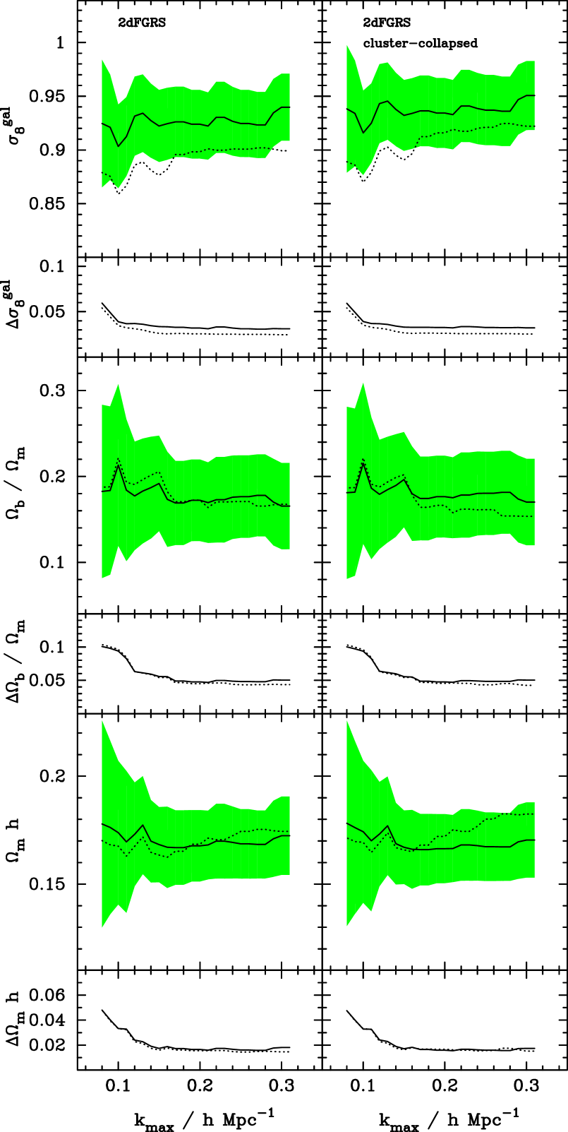
8.3.1 Dependence on scale

Figure 24: Contour plots showing changes in the likelihood from the maximum of $2\Delta\ln{\cal L}=1.0,2.3,6.0,9.2$ for different parameter combinations for the redshift-space 2dFGRS power spectrum, assuming a $\Lambda$CDM cosmology with $h=0.72$ and $n_{\rm s}=1.0$. Dashed contours in all plots are as in Fig. 22 and were fitted for $0.02<k<0.20{\,h\,\rm Mpc^{-1}}$, marginalizing over $Q$. The open circle marks the maximum likelihood position for each 2d likelihood surface. The solid contours show the likelihood surfaces calculated with: a) a fixed covariance matrix calculated from log-normal catalogues with model power spectrum matched to the best-fit 2dFGRS value. b) $Q=0$ fixed, and fitting to a reduced $k$ range of $0.02<k<0.15{\,h\,\rm Mpc^{-1}}$. c) covariance matrix calculated from log-normal catalogues with parameters at the Hubble Volume values. d) covariance matrix calculated from jack-knife 2dFGRS power spectra. e) the cluster-collapsed 2dFGRS catalogue marginalizing over $4<Q<12$ instead of $0<Q<8$. f) the pre-Feb 2001 dataset, as used in P01, but reanalysed using the revised method. g) the red subsample of galaxies. h) the blue subsample of galaxies. For each plot, the solid circle marks the maximum likelihood position of these revised likelihood surfaces. See text for further details of each likelihood calculation.

Figure 25: continued

In order to test the robustness of recovered parameters to the scales probed, Fig. 23 shows marginalized values of $\Omega_{\rm m}h$ and $\Omega_{\rm b}/\Omega_{\rm m}$ as a function of $k_{\rm max}$ (i.e. fitting to data with $0.02<k<k_{\rm max}$), contrasting results assuming that the observed galaxy power spectrum is directly proportional to the linear matter power spectrum with results involving marginalization over $Q$ and a large-scale correction as described in Section 7. We also compare results from the original redshift-space data to those calculated after the clusters have been collapsed. For the redshift-space data, we find that including the $Q$ prescription makes very little difference to the recovered parameters for $k_{\rm max}\mathrel{\lower 2.58334pt\hbox{$\buildrel{\textstyle<}\over{\scriptstyle\sim}$}}0.15{\,h\,\rm Mpc^{-1}}$, confirming the premise of P01 (i.e. the solid and dotted lines in the left column are similar for $k_{\rm max}\mathrel{\lower 2.58334pt\hbox{$\buildrel{\textstyle<}\over{\scriptstyle\sim}$}}0.15{\,h\,\rm Mpc^{-1}}$). However, this is not true for smaller scales.

If we restrict ourselves to the assumption that the measured power spectrum reflects linear theory exactly (dotted lines) then there is a trend towards higher $\Omega_{\rm m}h$ and lower baryon fraction with increasing $k_{\rm max}$. This effect is especially marked for the data where the clusters have been collapsed. However, if we apply our hybrid correction with $Q$ being allowed to float, these variations disappear: the recovered parameters display no significant change when $k_{\rm max}$ is increased from $0.15{\,h\,\rm Mpc^{-1}}$ to $0.3{\,h\,\rm Mpc^{-1}}$. This suggests that the $Q$ prescription is able to capture the real distortions of the redshift-space power spectrum with respect to linear theory.

On the other hand, it should be noted that the errors initially fall with increasing $k_{\rm max}$, but beyond $k_{\rm max}\simeq 0.2{\,h\,\rm Mpc^{-1}}$ there is no further reduction in the error – there is little additional information in the small scale data about the shape of the linear power spectrum.

8.3.2 Dependence on other assumptions

In Fig. 24 we compare the default likelihood surface from Fig. 22 (dashed lines), with surfaces calculated using either different data, or with a revised method.

(a) The three plots in the top-left of this figure show the likelihood surface calculated using a fixed covariance matrix (solid lines). This change in the method by which the likelihood is estimated is discussed further in Section 8.1. The net effect here is very small.

(b) In the three contour plots in the top-right of this figure, we show likelihood surfaces fitting to $0.02<k<0.15{\,h\,\rm Mpc^{-1}}$ fixing $Q=0$, (i.e. not allowing for any correction for small-scale effects), but still including the large-scale correction. The constraints on the power spectrum normalization and $\Omega_{\rm m}h$ are consistent in the two cases. $\Omega_{\rm m}h$ increases by about 2%, and the baryon fraction increases by about 10%.

(c) The effect of calculating the log-normal catalogues with model parameters other than the best-fit parameters is shown in Fig. 24c. Here the solid contours relate to the parameters of the Hubble Volume simulation ($h=0.7$, $\Omega_{\rm m}=0.3$, $\Omega_{\Lambda}=0.7$, $\Omega_{\rm b}=0.04$ and $\sigma_{8}=0.9$). However, this change in the assumed covariance matrix does not induce a significant change in the recovered parameter values.

(d) Instead of directly using the log-normal catalogues to estimate the covariance matrix, we have also considered using the jack-knife resampling of the 2dFGRS data described in Section 6. The jack-knife estimate of the covariance matrix was unstable to direct inversion; as an alternative, we smoothed the fractional difference between the jack-knife and log-normal covariance matrices, and used this smoothed map to adjust the log-normal covariance matrix. This resulted in essentially negligible change in the likelihood contours.

(e) The bottom left part of Fig. 24 shows likelihood surfaces calculated after collapsing the clusters in the 2dFGRS dataset. The scales fitted are the same in both cases, and both surfaces were calculated after marginalizing over $Q$. The shapes of the surfaces are in excellent agreement.

(f) In Fig. 24f we compare the new likelihood surface with that calculated using pre-Feb 2001 data. Rather than using the P01 data and covariance matrix, we reanalyse the pre-Feb 2001 data with our new method. We see that most of the difference between the result of P01 ($\Omega_{\rm m}h=0.20\pm 0.03$, $\Omega_{\rm b}/\Omega_{\rm m}=0.15\pm 0.07$) and our current best-fit parameters comes from the larger volume now probed: the parameter constraints in this plot were calculated in the same way for both datasets. For an alternative comparison, Fig. 26 compares our current likelihood surface with that of P01 over an extended parameter range. This shows that, in addition to the tightening of the confidence interval on parameters, the high baryon fraction solution of P01 is now rejected at high confidence.

(g) & (h) In these panels we show likelihood surfaces for the two samples defined by splitting the catalogue at a rest frame colour of $({\rm b_{J}}-r_{\rm\scriptscriptstyle F})_{z=0}=1.07$. In contrast to the samples discussed in Section 5.3 and plotted in Fig. 15, we do not force the mean weight per unit redshift to be the same for both samples. The samples therefore sample different regions, and some of the difference will be caused by cosmic variance. In both cases, a consistent $\Omega_{\rm m}h\simeq 0.17$ is derived.

Figure 26: Likelihood contours as in Fig. 22, but now calculated using the data, covariance matrix and methodology of P01 (dashed lines). The cosmological model is as described in Section 8.2 (it differs from that of P01 because we fix $h=0.72$). However, we have chosen to plot the contours for an extended range of $\Omega_{\rm m}h$ to match the analysis of P01. For comparison, the solid contours show our new default parameter constraints.

Figure 27: Recovered marginalized parameters from 22 Hubble Volume mock catalogues, demonstrating our ability to recover the true input parameters from samples that accurately match the size and geometry of the 2dFGRS survey. The solid lines mark the true cosmological parameters and normalization of the Hubble Volume simulation, calculated from a large realization of galaxies covering the full Hubble Volume cube. Open circles mark the marginalized parameters recovered from mocks with $2(\ln{\cal L}_{\rm max}-\ln{\cal L}_{\rm true})<2.3$ (corresponding to mocks with recovered parameters less than 1$\sigma$ from the true values), open squares $2.3<2(\ln{\cal L}_{\rm max}-\ln{\cal L}_{\rm true})<6.0$ (1$\sigma$ to 2$\sigma$ from the true values), and open triangles $2(\ln{\cal L}_{\rm max}-\ln{\cal L}_{\rm true}>6.0$ ($>$2$\sigma$ from the true values). The solid circle marks the average recovered parameters from all of the mocks. a) for the redshift-space Hubble Volume mocks fitting to $0.02<k<0.20{\,h\,\rm Mpc^{-1}}$ marginalizing over $Q$. b) for the real-space Hubble Volume mocks. c) for the cluster-collapsed redshift-space mocks. d) for the redshift-space Hubble Volume mocks fitting to $0.02<k<0.15{\,h\,\rm Mpc^{-1}}$ with $Q=0$.

8.4 Fitting to the HV mocks

As a final test, we apply the full fitting machinery to a set of 22 mock catalogues drawn from the Hubble Volume simulation (see Section 4.2.1). As discussed above, the choice of a fixed covariance matrix has only a minor effect on the results, so we use a single covariance matrix to analyse all these mock surveys. This approach also has the advantage that it is easier to test directly whether the distribution of the recovered parameters from these catalogues is consistent with the predicted confidence intervals.

In Fig. 27 we plot the recovered marginalized parameters from different sets of 22 redshift-space, real-space and cluster collapsed Hubble Volume mock catalogues. In general, the distribution of $\Omega_{\rm m}h$ and $\Omega_{\rm b}/\Omega_{\rm m}$ values follows the general degeneracy of cosmological models which give parameter surfaces with the same approximate shape as shown in Fig. 22. There is no evidence for a strong bias in the recovered parameters, and we find that the average recovered parameters are close to the true values.

Because the Hubble Volume mocks do not have luminosity dependent bias and we analyse them with the FKP estimator, the normalisation we recover corresponds to the typical galaxies, which have a bias that is approximately $1.26$ higher that of $L_{*}$ galaxies. Also, the prescription for scale-dependent bias given by equation (23) does not accurately match the artificial bias put into the Hubble Volume mocks, and the recovered $\sigma_{8}$ values are seen to be slightly offset from the expected numbers. This effect is not significant and merely relates to the crude bias model (equation 20) used for the Hubble Volume mocks.

There is some evidence that the average recovered value of $\Omega_{\rm m}h$ is higher for the real-space catalogues than for the redshift-space catalogues. This reflects the slight difference in large-scale shape between real and redshift space power spectra observed in Fig. 11. Even so, this deviation is smaller than the 1$\sigma$ errors on the recovered parameters from an individual catalogue.

9 Summary and discussion

9.1 Results from the complete 2dFGRS

This paper has been devoted to a detailed discussion of the galaxy power spectrum as measured by the final 2dFGRS. We have deduced improved versions of the masks that describe the angular selection of the survey, and modelled the radial selection via a new empirical treatment of evolutionary corrections. We have carried out extensive checks of our methodology, varying assumptions in the treatment of the data and applying our full analysis method to realistic mock catalogues.

Based on these investigations, we are confident that the 2dFGRS power spectrum can be used to infer the matter content of the universe, via fitting to a CDM model. Assuming a primordial $n_{\rm s}=1$ spectrum and $h=0.72$, the best fitting model has $\chi^{2}/{\rm d.f.}=36/32$ and the preferred parameters are

$$\Omega_{\rm m}h=0.168\pm 0.016$$ (39)

and a baryon fraction

$$\Omega_{\rm b}/\Omega_{\rm m}=0.185\pm 0.046.$$ (40)

We have kept $n_{\rm s}$ and $h$ fixed so that the quoted errors reflect only the uncertainties that arises from the uncertainty in the shape of power spectrum and not additional uncertainties due the choice of $n_{\rm s}$ and $h$. However the values and errors are insensitive to the choice of $h$. Allowing 10% Gaussian uncertainty gives $\Omega_{\rm m}h=0.174\pm 0.019$ and $\Omega_{\rm b}/\Omega_{\rm m}=0.190\pm 0.053$.

These values represent in some respects an important change with respect to P01, who found $\Omega_{\rm m}h=0.20\pm 0.03$ and $\Omega_{\rm b}/\Omega_{\rm m}=0.15\pm 0.07$. Statistically, the shift in the preferred parameters is unremarkable. However, the precision is greatly improved, by nearly a factor 2. This reflects a substantial increase in the survey volume since P01, both because the survey sky coverage is 50% larger, and because our improved understanding of the selection function enables us to work to larger redshifts. In particular, the reduced error on the baryon fraction means that P01’s suggestion of a non-zero baryon content can now be regarded as a definite measurement. Our figure of $\Omega_{\rm b}/\Omega_{\rm m}=0.185\pm 0.046$ appears at face value to be a 4-$\sigma$ detection of baryon features, although this overstates the significance. The difference in $\chi^{2}$ between the best zero-baryon model and the best overall model is 6.3, so the likelihood ratio is $L=\exp(-6.3/2)$. This might suggest a probability for no baryons of $L/(1+L)=0.04$, but such a figure is too generous: for a Gaussian distribution, this value of $L$ would be a 2.5-$\sigma$ effect, with one-tailed probability of 0.006. It therefore seems fair to reject the zero-baryon hypothesis at about the 1% level.

It should be emphasised that the above statements depend on the theoretical framework of the $\Lambda$CDM model. This is important not only because the theory quantifies the relation between the baryon fraction and any features in the power spectrum, but because it constrains the allowed form of any baryon signature. What is impressive in our data is not simply that the results suggest departures from a smooth curve, but that these deviations occur in the locations expected from theory. It is this prior knowledge that gives the extra statistical power needed in order to reject a zero-baryon model with confidence.

Of course, proving that the universe contains baryons hardly ranks as a great novelty. It is an inevitable prediction of the $\Lambda$CDM model that the matter power spectrum should contain baryon features, and it has recently been confirmed directly that these should survive in the galaxy spectrum (Springel et al., 2005). The signature is much smaller than the corresponding acoustic oscillations in the CMB, so this measurement in no way competes with the CMB as a means of pinning down the baryon density. Nevertheless, by demonstrating a clearcut connection between the temperature fluctuations in the CMB and the present-day galaxy distribution, the identification of the baryon signal in the 2dFGRS provides an important verification of our fundamental model of structure formation.

9.2 Cosmological implications

The ability of the matter power spectrum to determine cosmological parameters in isolation is limited owing to the inherent physical degeneracies in the CDM model. As is well known, these can be overcome by combination with data on CMB anisotropies. The most striking success of this method to date has been the combination of the 2dFGRS results from P01 with the year-1 WMAP data (Spergel et al. 2003), the results of which were subsequently confirmed using the SDSS galaxy power spectrum by Tegmark et al. (2004). It is of interest to see how our earlier conclusions alter in the light of our new results. We have used the Markov-Chain Monte-Carlo (MCMC; Lewis & Bridle 2002) method to fit cosmological models to our new power-spectrum data combined with WMAP year 1 (Hinshaw et al. 2003) CMB data. For the choice of model, we adopted the philosophy of Percival et al. (2002), allowing $\Omega_{\rm m}$, $\Omega_{\rm b}$, $h$, $n_{\rm s}$, $\tau$, $\sigma_{8}$ and $\sigma_{8}^{\rm gal}$ to vary while assuming negligible neutrino contribution and a flat cosmology. The results, ignoring the normalization of the model power spectra, are as follows:

 

$${\Omega_{\rm m}}$$

  (41)

We see that using the new 2dFGRS result decreases $\Omega_{\rm m}$ by approximately 15% from the best-fit WMAP value of $\Omega_{\rm m}\simeq 0.27$. This change is easily understood because our new best-fit $\Omega_{\rm m}h=0.168$ is lower than that of P01. The CMB acoustic peak locations constrain $\Omega_{\rm m}h^{3}$, so to fit the new data requires a lower value of $\Omega_{\rm m}$ coupled with a higher value of $h$. Again, what is impressive is that the accuracy is significantly improved, breaking the 10% barrier on $\Omega_{\rm m}$. For comparison, The WMAP analysis in Spergel et al. (2003) achieved 15% accuracy on $\Omega_{\rm m}$. As a result, we are able to achieve a firm rejection of the common ‘concordance’ $\Omega_{\rm m}=0.3$ in favour of a lower value ($0.19<\Omega_{\rm m}<0.27$ at 95% confidence). This result demonstrates that large-scale structure measurements continue to play a crucial role in determining the cosmological model.

References

- (1)
- Arnouts et al. (1997) Arnouts S., de Lapparent V., Mathez G., Mazure A., Mellier Y., Bertin E., Kruszewski A., 1997, A&A Suppl., 124, 163
- Arnouts et al. (2001) Arnouts S., et al., 2001, A&A, 379, 740
- Baldry et al. (2004) Baldry, I.K., Glazebrook, K., Brinkmann, J., Ivezic, Z., Lupton, R.H., Nichol R.C., Szalay A.S., 2004, ApJ, 600, 681
- Ballinger, Heavens & Taylor (1995) Ballinger W.E., Heavens A.F., Taylor A.N., 1995, MNRAS, 276, L59
- Ballinger, Peacock & Heavens (1996) Ballinger W.E., Peacock J.A., Heavens A.F., 1996, MNRAS, 282, 877
- Baugh et al. (2004) Baugh C.M., et al., (The 2dFGRS Team) 2004, MNRAS, 351, L44
- Benson et al. (2000) Benson A.J., Baugh C.M., Cole S., Frenk C.S., Lacey C.G., 2000, MNRAS, 316, 107
- Blanton et al. (2003) Blanton M.R., Brinkmann J., Csabai I., Doi M., Eisenstein D., Fukugita M., Gunn J.E., Hogg D.W., Schlegel D.J., 2003, AJ, 125, 2348 (http://cosmo.nyu.edu/mb144/kcorrect)
- Bond & Szalay (1983) Bond J.R., Szalay A.S., 1983, ApJ, 274, 443
- Bruzual & Charlot (1993) Bruzual A.G., Charlot S., 1993, ApJ, 405, 538
- Bruzual & Charlot (2003) Bruzual A.G., Charlot S., 2003, MNRAS, 344, 1000
- Busswell et al. (2004) Busswell G.S., Shanks T., Outram, P.J., Frith W.J., Metcalfe N., Fong R., 2004, MNRAS, 354, 991
- Cole et al. (1998) Cole S., Hatton S.J., Frenk C.S., Weinberg D.H. 1998, MNRAS 300, 945
- Coles & Jones (1991) Coles P., Jones B., 1991, MNRAS, 248, 1
- Colless et al. (2001) Colless M., et al., (The 2dFGRS Team) 2001, MNRAS, 328, 1039
- Colless et al. (2003) Colless M., et al., (The 2dFGRS Team) 2003, astro-ph/0306581
- Collister & Lahav (2005) Collister, A.A., Lahav, O., 2005, MNRAS, in press (astro-ph/0412516)
- Cooray (2004) Cooray A., 2004, MNRAS, 348, 250
- Cooray & Sheth (2002) Cooray A., Sheth, R., 2002, Physics Reports, 372, 1
- Croton et al. (2004) Croton D.J. et al., (The 2dFGRS Team) 2004, MNRAS, 352, 1232
- Dickinson et al. (2004) Dickinson C., et al., 2004, MNRAS, 353, 732
- Efstathiou et al. (1985) Efstathiou G., Davis M., White S.D.M., Frenk C.S., 1985, ApJS, 57, 241
- Efstathiou et al. (1990) Efstathiou G., Sutherland, W.J., & Maddox, S.J., 1990, Nature, 348, 705
- Efstathiou et al. (1992) Efstathiou G., Bond J.R., White, S.D.M., 1992, MNRAS, 258, P1
- Efstathiou et al. (2001) Efstathiou G., Moody S.J., 2001, MNRAS, 325, 1603
- Eisenstein & Hu (1998) Eisenstein D.J., Hu W., 1998, ApJ, 496, 605
- Eke et al. (2004) Eke V.R., et al., (The 2dFGRS Team) 2004, MNRAS, 348, 866
- Elgaroy et al. (2002) Elgaroy O., et al., (The 2dFGRS Team) 2002, PRL, 89, 061301
- Erdogdu et al. (2004) Erdogdu, P. et al., (The 2dFGRS Team) 2004, MNRAS, 352, 939
- Evrard et al. (2002) Evrard A.E., et al., 2002 ApJ, 573, 7
- Feldman, Kaiser & Peacock (1994) Feldman H.A., Kaiser N., Peacock J.A., 1994, MNRAS, 426, 23
- Frith et al. (2003) Frith W.J., Busswell G.S., Fong R., Metcalfe N., Shanks T., 2003, MNRAS, 345, 1049
- Gott et al. (2005) Gott J.R., Jurić, M., Schlegel, D., Hoyle, F., Vogeley, M., Tegmark, M., Bahcall, N., Brinkmann, J., 2005, ApJ, 624, 463
- Hambly, Irwin & MacGillivray (2001) Hambly N.C., Irwin M.J., MacGillivray H.T., 2001, MNRAS, 326, 1295
- Hawkins et al. (2003) Hawkins E., et al., (The 2dFGRS Team) 2003, MNRAS, 346, 78
- Hinshaw et al. (2003) Hinshaw G., et al., 2003, ApJS, 148, 135
- Hockney & Eastwood (1981) Hockney R.W., Eastwood J.W., 1981, Computer simulation using particles, New York: McGraw-Hill
- Jarrett et al. (2000) Jarrett T.H., Chester T., Cutri R., Schneider S., Skrutskie M., Huchra, J.P., 2000, AJ, 119, 2498
- Jing, Mo & Börner (1998) Jing Y.P., Mo H.J., & Börner G., 1998, ApJ, 494, 1
- Kaiser (1987) Kaiser N. 1987, MNRAS, 227, 1
- Kauffmann et al. (2003) Kauffmann, G., et al., 2003, MNRAS, 341, 54
- Kayo, Taruya & Suto (2001) Kayo, I., Taruya, A., Suto, Y., 2001, ApJ, 561, 22
- Lahav et al. (2002) Lahav O., et al., (The 2dFGRS Team) 2002, MNRAS, 333, 961
- Lewis & Bridle (2002) Lewis A., Bridle S., 2002, Phys. Rev. D, 66, 103511
- Maddox et al. (1990) Maddox S.J., Sutherland W.J., Efstathiou G., Loveday J., Peterson B.A., 1990, MNRAS, 247, 1p
- Madgwick et al. (2002) Madgwick D.S., et al., (The 2dFGRS Team) 2002, MNRAS, 333, 133
- Madgwick et al. (2003) Madgwick D.S., et al., (The 2dFGRS Team) 2003, MNRAS, 344, 847
- Magliocchetti & Porciani (2003) Magliocchetti, M., Porciani, C., 2003, MNRAS, 346, 186
- Metcalfe, Fong & Shanks (1995) Metcalfe N., Fong, R., Shanks, T., 1995, MNRAS, 274, 769
- Neyman & Scott (1952) Neyman J., Scott E.L., 1952, ApJ. 116, 114
- Norberg et al. (2001) Norberg P., et al. (The 2dFGRS Team), MNRAS 2001, 328, 64.
- Norberg et al. (2002a) Norberg P., et al. (The 2dFGRS Team), MNRAS 2002a, 332, 827
- Norberg et al. (2002b) Norberg P., et al., (The 2dFGRS Team) 2002b, MNRAS, 336, 907
- Padilla & Baugh (2003) Padilla N.D., Baugh C.M., 2003, MNRAS, 343, 796
- Peacock & Dodds (1994) Peacock J.A., Dodds S.J., 1994, MNRAS, 267, 1020
- Peacock & Smith (2000) Peacock J.A., Smith R.E., 2000, MNRAS, 318, 1144
- Peebles & Yu (1970) Peebles P.J.E., Yu J.T., 1970, ApJ, 162, 815
- Peebles (1980) Peebles P.J.E., 1980, The Large Scale Structure of the Universe, Princeton University Press
- Peebles (1982) Peebles P.J.E., 1982, ApJ, 263, L1
- Percival et al. (2001) Percival W.J., et al., (The 2dFGRS Team) 2001, MNRAS, 327, 1297 (P01)
- Percival et al. (2002) Percival W.J., et al., (The 2dFGRS Team) 2002, MNRAS, 337, 1068
- Percival, Verde & Peacock (2004a) Percival W.J., Verde L., Peacock J.A., 2004a, MNRAS, 347, 645
- Percival et al. (2004b) Percival W.J., et al., (The 2dFGRS Team) 2004b, MNRAS, 353, 1201
- Percival (2005) Percival W.J., 2005, MNRAS, 356, 1168
- Prandoni et al. (1999) Prandoni I., et al., 1999, A&A 345, 448
- Press et al. (1992) Press W.H., Teukolsky S,A., Vetterling W.T., Flannery B.P., 1992, Numerical recipes in C. The art of scientific computing, Second edition, Cambridge: University Press.
- Saunders et al. (1990) Saunders W., Rowan-Robinson M., Lawrence A., Efstathiou G., Kaiser N., Ellis R.S., Frenk C.S., 1990, MNRAS, 242, 318
- Schlegel et al. (1998) Schlegel D.J., Finkbeiner D.P., Davis M., 1998, ApJ, 500, 525
- Seljak (2000) Seljak U., 2000, MNRAS, 318, 203
- Seljak (2001) Seljak U., 2001, MNRAS 325, 1359
- Silk (1968) Silk J., 1968, ApJ, 151, 459
- Smith et al. (2003) Smith R.E., et al., 2003, MNRAS, 341, 1311
- Spergel et al. (2003) Spergel D.N., 2003, ApJS, 148, 175
- Springel et al. (2005) Springel, V. et al. 2005, Nature, 435, 572 (astro-ph/0504097)
- Stoughton et al. (2002) Stoughton C., et al., 2002, AJ, 123, 485
- Strateva et al. (2001) Strateva, I., et al., 2001, AJ, 122, 1861
- Sugiyama (1995) Sugiyama N., 1995, ApJS, 100, 281
- Sunyaev & Zeldovich (1970) Sunyaev R.A., Zeldovich Ya.B., 1970, Astrophys. & Space Science, 7, 3
- Tadros et al. (1999) Tadros H., et al., 1999, MNRAS, 305, 527
- Tegmark et al. (2002) Tegmark M., Hamilton A.J.S., Xu Y., 2002, MNRAS, 335, 887
- Tegmark et al. (2004) Tegmark M., et al., 2004, ApJ, 606, 702
- Tegmark et al. (2005) Tinker J.L., Weinberg D.H., Zheng Z., Zehavi I., 2005, ApJ in press. (astro-ph/0411777)
- Van den Bosch, Yang & Mo (2003) Van den Bosch, F.C., Yang X., Mo H.J, 2003, MNRAS, 340, 771
- Verde et al. (2002) Verde L., et al., (The 2dFGRS Team) 2002, MNRAS, 335, 432
- White et al. (1993) White S.D.M., Navarro J.F., Evrard A.E., Frenk, C.S., 1993, Nature, 366, 429
- White (2001) White M., 2001, MNRAS, 321, 1
- Wild et al. (2005) Wild, V., et al, (The 2dFGRS Team), 2005, MNRAS, 356, 247
- Zheng et al. (2005) Zheng Z., et al. 2005, ApJ in press. (astro-ph/0408564)