Modeling CHANDRA Low Energy Transmission Grating Spectrometer Observations of Classical Novae with PHOENIX

Abstract

We use the PHOENIX code package to model the X–ray spectrum of Nova V4743 Sagittarii observed with the LETGS onboard the Chandra satellite on 19 March 2003. To analyze nova atmospheres and related systems with an underlying nuclear burning envelope at X–ray wavelengths, it was necessary to update the code with new microphysics. We demonstrate that the X–ray emission is dominated by thermal bremsstrahlung and that the hard X–rays are dominated by Fe and N absorption. Preliminary models are calculated assuming solar abundances. It is shown that the models can be used to determine element abundances in the nova ejecta by increasing the absorption in the shell.

1 Introduction

We have modeled X–ray spectra of classical novae (CNe) with the PHOENIX–code version 13 Petz et al. (2004). With our models it is possible to determine the effective temperature of the nova atmosphere and the formation of X–ray emission in the nova shell. We show that it is possible to determine the abundances of the ejecta by modelling X–ray spectra of CNe and present our first results for the abundances of C, N, and O.

For the comparison of our model with observations we use an X–ray spectrum of Nova V4743 Sagittarii (Sgr) observed with the LETGS onboard the Chandra satellite in March 2003 Ness et al. (2003).

2 Modeling nova atmospheres in X–rays with PHOENIX

Our model atmospheres are 1D spherical symetric, expanding, and time independent. The radiative equilibrium is solved in the comoving frame and the radiative transfer is treated as special relativistic for an atmosphere in full NLTE with line blanketing of 8534 atomic levels from H, He, C, N, O, Ne, Mg, and Fe. We use an exponential density law ($\rho(r)\propto r^{-n}$) with a gradient of $n=3$ and a standard velocity field ($v(r)=\dot{M}/4\pi r^{2}\rho(r)$ , $\dot{M}$ = const) with an outer velocity of $v_{\rm out}=2500$ km s^-1.

The earlier versions of PHOENIX used atomic data from CHIANTI Version 3 (CHIANTI3) and the line lists of Kurucz. For this work, we have implemented two new atomic databases, CHIANTI Version 4 (CHIANTI4) Young et al. (2003) and APED, because the old databases did not provide enough data for the X–ray energy range. Using the new databases, we have extended PHOENIX to use many new spectral lines in the X–ray waveband down to 1 Å, improved data for electron collision rates, new data for proton collision rates, and better data for thermal bremsstrahlung.

3 X–ray observations of nova V4743 Sgr

The solid curve of Fig. 1 shows the observed X–ray spectrum of nova V4743 Sgr on March 19, 2003 with the LETGS onboard the CHANDRA satellite Ness et al. (2003). At wavelengths greater than $\approx 55$ Å, it is dominated by second and higher dispersion orders, and these wavelengths will not be considered in our analysis. The effective areas used to convert from ct s^-1 to flux are determined with the CIAO software package, version 3.0.

An examination of the spectrum shows that it is not a black–body but resembles a stellar atmosphere with deep absorption features and, possibly, some weak emission lines. The strongest lines are from the two highest ionisation stages of C, N, and O. An extensive analysis of the observation has been carried out by Ness et al. (2003).

4 Model with solar abundances

The best fit with solar abundances to the spectrum of nova V4743 Sgr is shown in Fig. 1, left panel. The model has an effective temperature of $T_{\rm eff}=5.8\times 10^{5}$ K and a bolometric luminosity of $L_{\rm bol}=50,000L_{\odot}$. To get the correct slope for the pseudo–continuum, a value of $n_{h}=4.0\times 10^{21}$ cm^-2 for the hydrogen column density has to be used. The quality of the fit is independent of the luminosity of the model. This was already found for earlier solar models in other wavelength ranges Hauschildt & Starrfield (1995).

Close inspection of the measured spectrum reveals that some spectral lines are not reproduced well or are missing in the model spectrum. This is because we have used only solar abundances in this model and have not increased abundances of, for example the CNO elements, as is generally observed in novae and predicted by theory Starrfield et al. (1998). Furthermore all absorption lines are too weak and there is too much emission around $\lambda\sim 24$ Å. Increasing the abundances should increase the absorption and the fit should improve with solar abundances.

The X–ray emission is dominated by thermal bremsstrahlung from the atmosphere surrounding the WD and the hard spectral range of $\lambda\lesssim 29$ Å is dominated by iron and nitrogen absorption. The atmosphere is in strong departure from LTE and is very extended with the highest ionization stages of elements in the outest layers.

5 Model with non–solar abundances

A model with non–solar abundances (Fig. 1, right panel) produces a spectrum which fits the observation much better than with solar abundances. It was calculated with a 22 times solar abundance of nitrogen and oxygen. Accordingly the nitrogen to oxygen ratio is equal to the solar value. The abundance of carbon with 1.25 times solar is only slightly higher than in solar material.

The strengths of some spectral lines now fit much better to the observation. For example, the fits of the N VII line at $\lambda\sim 24.8$ Å and the O VII line at $\lambda\sim 21.6$ Å. Around $\lambda\sim 24$ Å there is still too much emission.

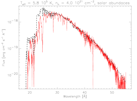
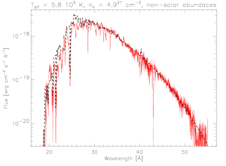
Figure 1: Model atmosphere of nova V4743 Sgr with solar (left) and non–solar abundances (right). The solid curve is the observed spectrum.

References

- Petz et al. (2004) Petz, A., Hauschildt, P. H., Ness, J. U., & Starrfield, S. 2004, AstroPh-0410370
- Ness et al. (2003) Ness, J. U., Starrfield, S., Burwitz, V., et al. 2003, ApJ, 594, L127
- Young et al. (2003) Young, P. R., Zanna, G. D., Landi, E., et al. 2003, ApJS, 144, 135
- Hauschildt & Starrfield (1995) Hauschildt, P. H. & Starrfield, S. 1995, ApJ, 447, 829
- Starrfield et al. (1998) Starrfield, S., Truran, J. W., Wiescher, M. C., & Sparks, W. M. 1998, MNRAS, 33, 804