The Weak Lensing Bispectrum

Abstract

Weak gravitational lensing of background galaxies offers an excellent opportunity to study the intervening distribution of matter. While much attention to date has focused on the two-point function of the cosmic shear, the three-point function, the bispectrum, also contains very useful cosmological information. Here, we compute three corrections to the bispectrum which are nominally of the same order as the leading term. We show that the corrections are small, so they can be ignored when analyzing present surveys. However, they will eventually have to be included for accurate parameter estimates from future surveys.

I Introduction

Weak lensing offers cosmologists the opportunity to probe the distribution of mass in the universe Bartelmann and Schneider (2001). This prospect is so alluring because theories make first-principles predictions about this distribution, so we can hope to extract important constraints on fundamental cosmological parameters from weak lensing surveys Benabed and Bernardeau (2001); Hu (2002); Huterer (2002); Abazajian and Dodelson (2003); Refregier et al. (2004); Simon et al. (2003); Bernstein and Jain (2004); Heavens (2003); Takada and Jain (2004). In many senses, this promise is similar to that felt by those who studied the cosmic microwave background (CMB) a decade ago: theoretical predictions are straightforward; experiments have detected the effect (anisotropies in that case and cosmic shear in this); and there are grand plans for the future (which have been realized in the case of the CMB).

Armed with this optimism, cosmologists are quick to throw in warning labels: the signal is extremely small, so the only way to measure cosmic shear is to average over many background galaxies. Each individual galaxy is observed with its own set of systematics (seeing, elliptical point spread functions, calibration, unknown or at least uncertain redshift, etc.) and these vary from one galaxy to another. Measurements of cosmic shear are unlikely to produce smooth maps since there inevitably will be bright stars which must be masked out. Accounting for these masks leads to complicated window functions. It is not clear then that weak lensing measurements will eventually pay off as did those of the CMB.

There is one area though in which weak lensing measurements have an advantage over the CMB: the higher point functions of the cosmic shear field are potentially simpler to interpret and more relevant than those in the CMB. Naively, this is what one would expect, for the cosmic shear field is sensitive to the matter density which has gone nonlinear and therefore will have large corrections to the Gaussian limit. Temperature fluctuations on the other hand are still stuck at the $10^{-5}$ level, so are expected to be very close to Gaussian (recall that the initial distribution of both temperature and matter inhomogeneities was likely Gaussian and for a Gaussian distribution the higher point functions are trivially related to the two-point function). We might expect then the 3-point function of CMB anisotropies to be very small, while that of the cosmic shear to be quite large, at least on small scales. Much work has been done over the past few years attempting to debunk these naive ideas. We have found that the higher point functions of the CMB are quite interesting: lensing Zaldarriaga (2000); Zaldarriaga and Seljak (1999); Hu (2001), hot gas Sunyaev and Zeldovich (1980a), peculiar velocities Sunyaev and Zeldovich (1980b), and reionization Cooray and Hu (2000); Castro (2003) leave their imprint in these higher point functions. Nonetheless, the fact remains that to date there has been no detection of a non-zero 3-point function, for example, in the CMB, while several groups Bernardeau et al. (2002a); Pen et al. (2003) have claimed such a detection in the cosmic shear field. Further, a number of authors Hui (1999); Benabed and Bernardeau (2001); Cooray and Hu (2001); Refregier et al. (2004); Takada and Jain (2004) have showed that the bispectrum of the cosmic shear field will be able to constrain important cosmological parameters, including properties of the dark energy. Certainly, then, we need to obtain accurate predictions of the bispectrum of the shear.

With this in mind, it is important to emphasize just how important “higher order” corrections to the bispectrum might be. To understand this, recall that, to lowest order, the shear is a line-of-sight integral over the matter overdensity:

$$\gamma({\bf\theta})=\int d\chi f(\chi)\delta({\bf x}(\chi,{\bf\theta}))$$ (1)

where ${\bf\theta}$ is the angular position on the sky, $f$ is a weighting function, and $\chi$ is the comoving distance along the line of sight. Roughly then the bispectrum, which is proportional to $\langle\gamma^{3}\rangle$, is proportional to $\langle\delta^{3}\rangle$. It vanishes therefore in the large-scale limit where the density field is Gaussian and nonlinearities are irrelevant. The main contribution to the bispectrum then comes from the fact that, due to gravity, $\delta$ evolves nonlinearly. In perturbation theory, we would write $\delta=\delta^{(1)}+\delta^{(2)}+\ldots$ where $\delta^{(1)}$ is the linear overdensity and $\delta^{(2)}$ is proportional to $\delta_{L}^{2}$. This main contribution to the bispectrum then comes from terms proportional to $\langle\delta^{(1)}\delta^{(1)}\delta^{(2)}\rangle$ and so is proportional to $\delta_{L}^{4}$.

It is clear then that any correction which alters the linear relation between shear and overdensity in Eq. (1) is of the same order in $\delta_{L}$ as the “main contribution.” Here we study three such corrections first identified by Schneider et al. Schneider et al. (1998) and compute their effect on the bispectrum:

• Reduced Shear We estimate shear by measuring ellipticities of background galaxies, invoking the relation Bartelmann and Schneider (2001); Dodelson (2003) $\epsilon_{i}=2\gamma_{i}$, where the subscript $i$ refers to the two components of ellipticity/shear. This relation though is only approximate; the full relation is

  $$\epsilon_{i}={2\gamma_{i}\over 1-\kappa}$$ (2)

  where $\kappa$ is the convergence. Expanding the denominator, we see that the ellipticities used to estimate cosmic shear have terms quadratic in the perturbations ($2\gamma_{i}\kappa$). This quadratic term contributes to the bispectrum at the same order as the main term.

• Lens-Lens Coupling Eq. (1) does not account for the fact that lenses are correlated along the line of sight. This lens-lens coupling induces another quadratic term in the relation between shear and overdensity.

• Born Approximation When computing the shear one integrates along the photon path back towards the source. There is a complication inherent in this integration encoded in the argument of the overdensity in Eq. (1): what is the position of the photon at radial distance $\chi$ if its observed angular position today is ${\bf\theta}$? the naive answer ${\bf x}^{(0)}=\chi({\bf\theta},1)$ is the position corresponding to the path taken by an undeflected photon. Expanding about this zero order position leads to a correction proportional to $\nabla\delta\cdot[{\bf x}-{\bf x}^{(0)}]$. Since ${\bf x}$ differs from the undeflected position only if $\delta$ is nonzero, this correction is second order in $\delta$. It too contributes a term of order $\delta^{4}$ to the bispectrum.

The next section reviews some basic lensing results including the standard computations of the power spectrum and the bispectrum. §III computes the correction to the bispectrum from the three effects enumerated above. The bispectrum cannot be simply plotted on a 2D graph since it depends on the three variables required to specify a triangle. Therefore, §IV examines various ways of condensing the information contained in these corrections. The goal is to see whether the corrections are important.

II Review of Basic Results

The deformation tensor is defined as the deviation from unity of the Jacobian relating the undeflected position (${\bf\theta_{S}}$) to the actual position (${\bf\theta}$):

$$\psi_{ij}\equiv\delta_{ij}-{\partial\theta_{S,i}\over\partial\theta_{j}}.$$ (3)

The elements of this $2\times 2$ matrix are the two components of shear and the convergence:

$$\psi_{ij}\equiv\left(\matrix{\kappa+\gamma_{1}&\gamma_{2}\cr\gamma_{2}&\kappa-\gamma_{1}}\right).$$ (4)

These are simply definitions. The physics comes from solving the geodesic equation and expressing the distortion tensor in terms of the gravitational potential $\Phi$:

$$\psi_{ij}({\bf\theta},\chi_{s})=\int_{0}^{\chi_{s}}d\chi W(\chi,\chi_{s}){\partial^{2}\Phi\left({\bf x}({\bf\theta},\chi);\chi\right)\over\partial x_{i}\partial x_{k}}\left[\delta_{kj}-\psi_{kj}({\bf\theta},\chi)\right].$$ (5)

Here, we are assuming a flat universe; sources are assumed to lie at $\chi_{s}$; the first argument of the $\Phi$ is the 3D comoving position (in the small angle limit)

$${\bf x}({\bf\theta},\chi)=[\chi\theta_{x},\chi\theta_{y},\chi]-\int_{0}^{\chi}d\chi^{\prime}W(\chi^{\prime},\chi){\chi\over\chi^{\prime}}\nabla\Phi\left({\bf x}({\bf\theta},\chi^{\prime});\chi\right)$$ (6)

while the second ($\chi$) refers to the cosmic time at which the photon path passed by this position. The weighting function is

$$W(\chi,\chi_{s})=2\chi(1-\chi/\chi_{s})\Theta(\chi_{s}-\chi).$$ (7)

We observe ellipticities of background galaxies $\epsilon_{i}$, which are related to the elements of the distortion tensor via

$$\epsilon_{i}={2\gamma_{i}\over 1-\kappa}.$$ (8)

One way to estimate the convergence, which is the projected density, is to work in Fourier space; then,

$$\hat{\tilde{\kappa}}({\bf l})={1\over l^{2}}T_{i}({\bf l})\tilde{\epsilon}_{i}({\bf l}).$$ (9)

Here the variable conjugate to ${\bf\theta}$ is ${\bf l}$. As usual, large $l$ corresponds to small scales. The trigonometric functions in Eq. (9) are defined with respect to an arbitrary $x$- axis as

$$T_{1}({\bf l}) \equiv {l_{x}^{2}-l_{y}^{2}\over 2}={l^{2}\over 2}\cos(2\phi_{l})$$

$$T_{2}({\bf l}) \equiv l_{x}l_{y}={l^{2}\over 2}\sin(2\phi_{l}).$$ (10)

Here $\phi_{l}$ is the angle between ${\bf l}$ and the $x$- axis. In the limit in which $\epsilon_{i}\rightarrow 2\gamma_{i}$, the estimator in Eq. (9) reduces to

$$\hat{\tilde{\kappa}}({\bf l}) \overbrace{\longrightarrow}^{\rm reduced\ shear} \cos(2\phi_{l})\tilde{\gamma}_{1}({\bf l})+\sin(2\phi_{l})\tilde{\gamma}_{2}({\bf l})$$ (11)

$$= \cos(2\phi_{l})(\tilde{\psi}_{11}({\bf l})-\tilde{\psi}_{22}({\bf l}))/2+\sin(2\phi_{l})\tilde{\psi}_{12}({\bf l})$$

$$\overbrace{\longrightarrow}^{\rm lens-lens} {-l^{2}\over 2}\tilde{\psi}({\bf l}).$$

The approximation on the first line neglects the fact that ellipticities are sensitive to the reduced shear; the approximation on the third line neglects the second order term in the brackets in Eq. (5), the term which accounts for the fact that the lens distribution is correlated. The projected potential in Eq. (11) is defined as

$$\psi({\bf\theta},\chi_{s})=\int_{0}^{\chi_{s}}d\chi{W(\chi,\chi_{s})\over\chi^{2}}\Phi\left({\bf x}({\bf\theta},\chi);\chi\right).$$ (12)

In the Born approximation the gravitational potential in the integral along the line of sight is evaluated at the unperturbed path. In that case, its Fourier transform reduces to

$$\tilde{\psi}({\bf l},\chi_{s})\overbrace{\longrightarrow}^{\rm Born}\tilde{\psi}^{(0)}({\bf l},\chi_{s})=\int_{0}^{\chi_{s}}d\chi{W(\chi,\chi_{s})\over\chi^{2}}\tilde{\phi}\left({\bf l};\chi\right)$$ (13)

with

$$\tilde{\phi}({\bf l},\chi)\equiv{1\over\chi^{2}}\int{dk_{3}\over 2\pi}\tilde{\Phi}({\bf l}/\chi,k_{3};\chi)e^{ik_{3}\chi}.$$ (14)

Note that $\tilde{\phi}$ is dimensionless unlike $\tilde{\Phi}$ which has dimensions of (length)³.

The statistics of $\tilde{\psi}^{(0)}$ follow directly from those of $\tilde{\phi}$, which are simple if we include only modes with $k_{3}$ small, i.e. the Limber approximation Limber (1954); Dodelson (2003),

$$\langle\tilde{\phi}({\bf l},\chi)\tilde{\phi}({\bf l}^{\prime},\chi^{\prime})\rangle=(2\pi)^{2}\delta^{2}({\bf l}+{\bf l}^{\prime})\delta(\chi-\chi^{\prime})P_{\Phi}(l/\chi;\chi)/\chi^{2}.$$ (15)

Here $P_{\Phi}$ is the power spectrum of the gravitational potential. Similarly, the three point-function is related to the spatial bispectrum Castro (2003):

$$\langle\tilde{\phi}({\bf l}_{1},\chi_{1})\tilde{\phi}({\bf l}_{2},\chi_{2})\tilde{\phi}({\bf l}_{3},\chi_{3})\rangle=(2\pi)^{2}\delta^{2}({\bf l}_{1}+{\bf l}_{2}+{\bf l}_{3})\delta(\chi-\chi^{\prime})\delta(\chi-\chi^{\prime\prime})B_{\Phi}({\bf l}_{1}/\chi,{\bf l}_{2}/\chi,{\bf l}_{3}/\chi;\chi)/\chi^{4}.$$ (16)

Then, we have

$$\langle\tilde{\psi}^{(0)}({\bf l})\tilde{\psi}^{(0)}({\bf l}^{\prime})\rangle=(2\pi)^{2}\delta^{2}({\bf l}+{\bf l}^{\prime})P_{2}(l),$$ (17)

with

$$P_{2}(l)=\int_{0}^{\infty}d\chi{W^{2}(\chi,\chi_{s})\over\chi^{6}}P_{\Phi}(l/\chi;\chi).$$ (18)

Similarly, the three-point function is

$$\langle\tilde{\psi}^{(0)}({\bf l}_{1})\tilde{\psi}^{(0)}({\bf l}_{2})\tilde{\psi}^{(0)}({\bf l}_{3})\rangle=(2\pi)^{2}\delta^{2}({\bf l}_{1}+{\bf l}_{2}+{\bf l}_{3})P_{3}({\bf l}_{1},{\bf l}_{2},{\bf l}_{3}),$$ (19)

where now the projected power is a line-of-sight integral over the bispectrum:

$$P_{3}({\bf l}_{1},{\bf l}_{2},{\bf l}_{3})=\int_{0}^{\infty}d\chi{W^{3}(\chi)\over\chi^{10}}B_{\Phi}({\bf l}_{1}/\chi,{\bf l}_{2}/\chi,{\bf l}_{3}/\chi;\chi).$$ (20)

The power spectrum, or the $C_{l}$’s, are defined as the coefficient of $(2\pi)^{2}\delta({\bf l}+{\bf l}^{\prime})$ when computing the variance of $\hat{\tilde{\kappa}}$. Since $\hat{\tilde{\kappa}}=-l^{2}\psi^{(0)}/2$ in the standard computation, we have

$$C^{\kappa}_{l}=l^{4}P_{2}(l)/4.$$ (21)

Similarly, the bispectrum of the $\kappa$ estimator is

$$B^{\kappa}({\bf l}_{1},{\bf l}_{2},{\bf l}_{3})=-l^{6}P_{3}({\bf l}_{1},{\bf l}_{2},{\bf l}_{3})/8,$$ (22)

in agreement with previous results Takada and Jain (2004). The bispectrum with all $l$’s equal, the equilateral configuration, is shown in Fig. 1.

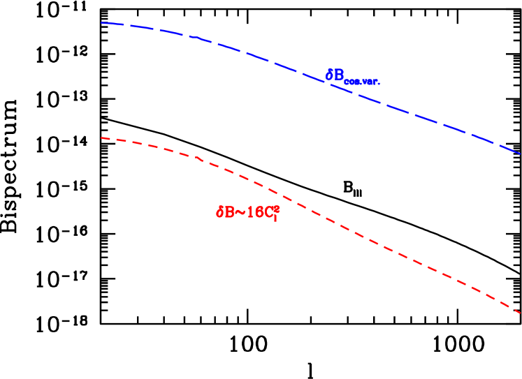
Figure 1: Equilateral bispectrum. Solid curve is the standard result; short-dashed [red] curve is order of magnitude of corrections considered here; long-dashed [blue] curve is cosmic-variance error. The signal to noise from a single configuration is therefore extremely small.

A few qualitative comments are in order here. The standard measure of the amplitude of fluctuations is $l^{2}C_{l}^{\kappa}=l^{6}P_{2}/4$. Let’s do an order of magnitude estimate for this quantity $l^{6}P_{2}$ in terms of the amplitude of density fluctuations, $\Delta^{2}\equiv k^{3}P_{\delta}/2\pi^{2}$. Since $l\sim(k/H_{0})$ and since $\Phi\sim(H_{0}/k)^{2}\delta$, we have $P_{\Phi}\sim P_{\delta}/l^{4}$. Now, Eq. (18) suggests that $P_{2}\sim P_{\Phi}/\chi^{3}$; since $\chi\sim l/k$, $P_{2}\sim(k/l)^{3}P_{\Phi}\sim(k/l)^{3}P_{\delta}/l^{4}\sim\Delta^{2}/l^{7}$. We expect then that $l^{6}P_{2}$ should be of order $\Delta^{2}/l$. What this means physically is that projection effects suppress the 2D power spectrum by a factor of $1/l$. There is even a nice explanation of this in terms of Fourier modes Kaiser (1992); Dodelson (2003): only modes with small $k_{3}$ contribute; these are a fraction of $1/l$ of the total number of modes. The bottom line then is that the power spectrum of the convergence is smaller than the power spectrum of the 3D density field.

Similar order of magnitude estimates relate the angular bispectrum, $-l^{6}P_{3}/8$, to the 3D bispectrum of the density field:

$$l^{6}P_{3}\sim l^{6}\left[(k/l)^{6}B_{\Phi}\right]\sim H_{0}^{6}B_{\delta}.$$ (23)

The corrections we consider below are all of order $l^{8}P_{2}^{2}$, which by the arguments of the preceding paragraph are of order $H_{0}^{6}P_{\delta}^{2}$. The 3D bispectrum $B_{\delta}$ is nominally of the same order as the square of the power spectrum, $P_{\delta}^{2}$. However, numerically it is a bit larger Bernardeau et al. (2002b), as indicated in Fig. 1, so the corrections we compute are not as important as we would have hoped.

III Higher Order Terms

We now compute the corrections to the bispectrum from going beyond the approximations in Eq. (11) and Eq. (13).

III.1 Reduced Shear

The first-order correction to the $\epsilon-\gamma$ relation is

$$\epsilon_{i}^{\rm rs}=2\gamma_{i}\kappa.$$ (24)

When we switch to Fourier space, the relation between ellipticity and shear is a convolution integral (products in real space correspond to convolutions in Fourier space):

$$\tilde{\epsilon}_{i}^{\rm rs}({\bf l})=\int{d^{2}l^{\prime}\over(2\pi)^{2}}l^{\prime 2}T_{i}({\bf l}-{\bf l}^{\prime})\tilde{\psi}^{(0)}({\bf l}^{\prime})\tilde{\psi}^{(0)}({\bf l}-{\bf l}^{\prime})$$ (25)

When we form the bispectrum of the $\kappa$ estimator (Eq. (9)), the first order correction emerges by replacing one of the three ellipticities with the higher order Eq. (25). So this correction to the bispectrum estimator becomes:

$$\langle\hat{\tilde{\kappa}}({\bf l}_{1})\hat{\tilde{\kappa}}({\bf l}_{2})\hat{\tilde{\kappa}}({\bf l}_{3})\rangle^{\rm rs} = {T_{i}({\bf l}_{1})l_{2}^{2}l_{3}^{2}\over 4l_{1}^{2}}\int{d^{2}l^{\prime}\over(2\pi)^{2}}l^{\prime 2}T_{i}({\bf l}_{1}-{\bf l}^{\prime})\langle\tilde{\psi}^{(0)}({\bf l}^{\prime})\tilde{\psi}^{(0)}({\bf l}_{1}-{\bf l}^{\prime})\tilde{\psi}^{(0)}({\bf l}_{2})\tilde{\psi}^{(0)}({\bf l}_{3})\rangle$$ (26)

$$+\left({\bf l}_{1}\leftrightarrow{\bf l}_{2}\right)+\left({\bf l}_{1}\leftrightarrow{\bf l}_{3}\right).$$

The four-point function for the potential gets contributions from the connected part – the trispectrum – and the disconnected part: the product of power spectra. Here we consider only the latter set of terms as these are expected to dominate. That is, let

$$\langle\tilde{\psi}^{(0)}({\bf l}^{\prime})\tilde{\psi}^{(0)}({\bf l}_{1}-{\bf l}^{\prime})\tilde{\psi}^{(0)}({\bf l}_{2})\tilde{\psi}^{(0)}({\bf l}_{3})\rangle \rightarrow (2\pi)^{4}P_{2}({\bf l}_{2})P_{2}({\bf l}_{3})$$

$$\times\Big{[}\delta^{2}({\bf l}^{\prime}+{\bf l}_{2})\delta^{2}({\bf l}_{1}-{\bf l}^{\prime}+{\bf l}_{3})+\delta^{2}({\bf l}^{\prime}+{\bf l}_{3})\delta^{2}({\bf l}_{1}-{\bf l}^{\prime}+{\bf l}_{2})\Big{]}.$$

The integral over ${\bf l}^{\prime}$ then leaves the coefficient of $(2\pi)^{2}\delta^{2}({\bf l}_{1}+{\bf l}_{2}+{\bf l}_{3})$ as

$${T_{i}({\bf l}_{1})l_{2}^{2}P_{2}(l_{2})l_{3}^{2}P_{2}(l_{3})\over 4l_{1}^{2}}\left[l_{2}^{2}T_{i}({\bf l}_{3})+l_{3}^{2}T_{i}({\bf l}_{2})\right]$$ (28)

plus permutations. The contraction over the geometric factors involves

$$T_{i}({\bf l}_{1})T_{i}({\bf l}_{2})={l_{1}^{2}l_{2}^{2}\over 4}\cos(2\phi_{12})$$ (29)

where $\phi_{12}$ is the angle between ${\bf l}_{1}$ and ${\bf l}_{2}$.

Defining $B_{123}\equiv B({\bf l}_{1},{\bf l}_{2},{\bf l}_{3})$ as the coefficient multiplying $(2\pi)^{2}\delta^{2}({\bf l}_{1}+{\bf l}_{2}+{\bf l}_{3})$, we therefore have

$$B_{123}^{\rm rs}={l_{2}^{4}l_{3}^{4}P_{2}(l_{2})P_{2}(l_{3})\over 16}\left[\cos(2\phi_{13})+\cos(2\phi_{12})\right]$$ (30)

plus permutations.

III.2 Lens-Lens Coupling

Lens-lens coupling in encapsulated by the second term in square brackets in Eq. (4). This contribution to the distortion tensor is then

$$\psi^{\rm ll}_{ab}({\bf\theta},\chi_{s})=-\int d\chi W(\chi,\chi_{s})\Phi_{,ac}\psi_{cb}({\bf\theta},\chi).$$ (31)

At second order in $\Phi$, this reduces to

$$\psi^{\rm ll}_{ab}({{\bf\theta}},\chi_{s})=-\int d\chi W(\chi,\chi_{s})\Phi_{,ac}({\bf\theta},\chi)\int d\chi^{\prime}W(\chi^{\prime},\chi)\Phi_{,cb}({\bf\theta},\chi^{\prime}).$$ (32)

Using Eq. (9), we can compute how this term contributes to the estimator of convergence. The second-order contribution is

$$\hat{\kappa}^{\rm ll}({\bf l}) = {2T_{i}({\bf l})\gamma_{i}^{\rm ll}({\bf l})\over l^{2}}$$ (33)

$$= {-T_{i}({\bf l})\over l^{2}}\int{d^{2}l^{\prime}\over(2\pi)^{2}}E_{i}({\bf l}^{\prime},{\bf l}-{\bf l}^{\prime})\int{d\chi\over\chi^{2}}W(\chi,\chi_{s})\int{d\chi^{\prime}\over\chi^{\prime 2}}W(\chi^{\prime},\chi)\tilde{\phi}({\bf l}^{\prime},\chi)\tilde{\phi}({\bf l}-{\bf l}^{\prime},\chi^{\prime}).$$

Here the geometrical factors are defined as

$$E_{1}({\bf l}_{1},{\bf l}_{2}) \equiv {\bf l}_{1}\cdot{\bf l}_{2}\left[{\bf l}_{1,x}{\bf l}_{2,x}-{\bf l}_{1,y}{\bf l}_{2,y}\right]$$

$$E_{2}({\bf l}_{1},{\bf l}_{2}) \equiv {\bf l}_{1}\cdot{\bf l}_{2}\left[{\bf l}_{1,x}{\bf l}_{2,y}+{\bf l}_{1,y}{\bf l}_{2,x}\right].$$ (34)

The estimator for the bispectrum of the convergence then gets a Gaussian contribution from the lens-lens term. One such term is

$$\langle\hat{\kappa}^{\rm ll}({\bf l}_{1})\hat{\kappa}^{(0)}({\bf l}_{2})\hat{\kappa}^{(0)}({\bf l}_{3})\rangle = {-l_{2}^{2}l_{3}^{2}T_{i}({\bf l}_{1})\over 4l_{1}^{2}}\int{d\chi\over\chi^{2}}W(\chi,\chi_{s})\int{d\chi^{\prime}\over\chi^{\prime 2}}W(\chi^{\prime},\chi)\int{d\chi_{2}\over\chi_{2}^{2}}W(\chi_{2},\chi_{s})\int{d\chi_{3}\over\chi_{3}^{2}}W(\chi_{3},\chi_{s})$$ (35)

$$\times\int{d^{2}l^{\prime}\over(2\pi)^{2}}E_{i}({\bf l}^{\prime},{\bf l}_{1}-{\bf l}^{\prime})\langle\tilde{\phi}({\bf l}^{\prime},\chi)\tilde{\phi}({\bf l}_{1}-{\bf l}^{\prime},\chi^{\prime})\tilde{\phi}({\bf l}_{2},\chi_{2})\tilde{\phi}({\bf l}_{3},\chi_{3})\rangle.$$

Two other terms exist with ${\bf l}_{1}\leftrightarrow{\bf l}_{2}$ and ${\bf l}_{1}\leftrightarrow{\bf l}_{3}$. In this case, the trispectrum does not contribute in the Limber approximation. Physically, the Limber approximation sets all lenses close to each other; mathematically, this corresponds to enforcing the constraint that the line of sight distances are all equal Castro (2003). Here this constraint sets $\chi=\chi^{\prime}=\chi_{2}=\chi_{3}$, so that $W(\chi^{\prime},\chi)$ vanishes. The only relevant terms therefore are the two products of two-point functions. Momentum conservation from the first such pair enforces ${\bf l}^{\prime}=-{\bf l}_{2}$ and ${\bf l}_{1}-{\bf l}^{\prime}=-{\bf l}_{3}$. Each two point function is evaluated using the Limber approximation as in Eq. (15).

The bispectrum from lens-lens coupling is then

$$B_{123}^{\rm ll} = {-l_{2}^{2}l_{3}^{2}T_{i}({\bf l}_{1})E_{i}({\bf l}_{2},{\bf l}_{3})\over 4l_{1}^{2}}\int{d\chi\over\chi^{6}}W^{2}(\chi,\chi_{s})\int{d\chi^{\prime}\over\chi^{\prime 6}}W(\chi^{\prime},\chi)W(\chi^{\prime},\chi_{s})$$ (36)

$$\times\left[P_{\Phi}(l_{2}/\chi;\chi)P_{\Phi}(l_{3}/\chi^{\prime};\chi^{\prime})+P_{\Phi}(l_{3}/\chi;\chi)P_{\Phi}(l_{2}/\chi^{\prime};\chi^{\prime})\right]+({\bf l}_{1}\leftrightarrow{\bf l}_{2})+({\bf l}_{1}\leftrightarrow{\bf l}_{3}).$$

Here we have used the fact that $E_{i}({\bf l}_{1},-{\bf l}_{2})=E_{i}({\bf l}_{1},{\bf l}_{2})=E({\bf l}_{2},{\bf l}_{1})$.

The geometrical factor in front reduces to

$$T_{i}({\bf l}_{1})E_{i}({\bf l}_{2},{\bf l}_{3})={l_{1}^{2}l_{2}^{2}l_{3}^{2}\cos(2\phi_{23})\over 2}\cos(\phi_{12}+\phi_{13}).$$ (37)

Therefore,

$$B_{123}^{\rm ll} = {-l_{2}^{4}l_{3}^{4}\cos(2\phi_{23})\cos(\phi_{12}+\phi_{13})\over 8}\int{d\chi\over\chi^{6}}W^{2}(\chi,\chi_{s})\int{d\chi^{\prime}\over\chi^{\prime 6}}W(\chi^{\prime},\chi)W(\chi^{\prime},\chi_{s})$$ (38)

$$\times\left[P_{\Phi}(l_{2}/\chi;\chi)P_{\Phi}(l_{3}/\chi^{\prime};\chi^{\prime})+P_{\Phi}(l_{3}/\chi;\chi)P_{\Phi}(l_{2}/\chi^{\prime};\chi^{\prime})\right]+({\bf l}_{1}\leftrightarrow{\bf l}_{2})+({\bf l}_{1}\leftrightarrow{\bf l}_{3}).$$

III.3 Born Approximation

The distortion tensor in Eq. (5) evaluates the potential everywhere along the unperturbed path of the light. To go beyond the Born approximation, we need to evaluate the potential at ${\bf x}={\bf x}_{0}+\delta{\bf x}$ where

$$\delta x_{a}({\bf\theta},\chi)=-\int d\chi^{\prime}W(\chi^{\prime},\chi){\chi\over\chi^{\prime}}\Phi_{,a}({\bf x}_{0};\chi^{\prime}).$$ (39)

This leads to a new contribution to the distortion tensor, which in Fourier space, reads

$$\tilde{\psi}^{\rm Born}_{ab}({\bf l},\chi_{s})=-\int{d\chi\over\chi^{2}}W(\chi,\chi_{s})\int{d\chi^{\prime}\over\chi^{\prime 2}}W(\chi^{\prime},\chi)\int{d^{2}l^{\prime}\over(2\pi)^{2}}l^{\prime}_{a}l^{\prime}_{b}l^{\prime}_{c}({\bf l}-{\bf l}^{\prime})_{c}\tilde{\phi}({\bf l}^{\prime};\chi)\tilde{\phi}({\bf l}-{\bf l}^{\prime};\chi^{\prime}).$$ (40)

This extra term in the distortion tensor contributes to the estimator for the convergence

$${\hat{\tilde{\kappa}}}^{\rm Born}={-T_{i}({\bf l})\over l^{2}}\int{d\chi\over\chi^{2}}W(\chi,\chi_{s})\int{d\chi^{\prime}\over\chi^{\prime 2}}W(\chi^{\prime},\chi)\int{d^{2}l^{\prime}\over(2\pi)^{2}}F_{i}({\bf l}^{\prime},{\bf l}-{\bf l}^{\prime})\tilde{\phi}({\bf l}^{\prime};\chi)\tilde{\phi}({\bf l}-{\bf l}^{\prime};\chi^{\prime}).$$ (41)

Here

$$F_{i}({\bf l}_{1},{\bf l}_{2})\equiv 2{\bf l}_{1}\cdot{\bf l}_{2}T_{i}({\bf l}_{1}).$$ (42)

This expression is identical in form to that from lens-lens coupling, with the substitution $E_{i}\rightarrow-F_{i}$. We can therefore copy the result from Eq. (36) to get

$$B_{123}^{\rm Born} = {-l_{2}^{2}l_{3}^{2}T_{i}({\bf l}_{1})\over 4l_{1}^{2}}\int{d\chi\over\chi^{6}}W^{2}(\chi,\chi_{s})\int{d\chi^{\prime}\over\chi^{\prime 6}}W(\chi^{\prime},\chi)W(\chi^{\prime},\chi_{s})$$ (43)

$$\times\left[P_{\Phi}(l_{2}/\chi;\chi)P_{\Phi}(l_{3}/\chi^{\prime};\chi^{\prime})F_{i}({\bf l}_{2},{\bf l}_{3})+P_{\Phi}(l_{3}/\chi;\chi)P_{\Phi}(l_{2}/\chi^{\prime};\chi^{\prime})F_{i}({\bf l}_{3},{\bf l}_{2})\right]+({\bf l}_{1}\leftrightarrow{\bf l}_{2})+({\bf l}_{1}\leftrightarrow{\bf l}_{3}).$$

But, $T_{i}({\bf l}_{1})F_{i}({\bf l}_{2},{\bf l}_{3})=l_{1}^{2}l_{2}^{3}l_{3}\cos(2\phi_{12})\cos(\phi_{23})$, so

$$B_{123}^{\rm Born} = {-l_{2}^{3}l_{3}^{3}\cos(\phi_{23})\over 8}\int{d\chi\over\chi^{6}}W^{2}(\chi,\chi_{s})\int{d\chi^{\prime}\over\chi^{\prime 6}}W(\chi^{\prime},\chi)W(\chi^{\prime},\chi_{s})$$ (44)

$$\times \left[l_{2}^{2}P_{\Phi}(l_{2}/\chi;\chi)P_{\Phi}(l_{3}/\chi^{\prime};\chi^{\prime})\cos(2\phi_{12})+l_{3}^{2}P_{\Phi}(l_{3}/\chi;\chi)P_{\Phi}(l_{2}/\chi^{\prime};\chi^{\prime})\cos(2\phi_{13})\right]+({\bf l}_{1}\leftrightarrow{\bf l}_{2})+({\bf l}_{1}\leftrightarrow{\bf l}_{3}).$$

III.4 Summary

Here we collect the results from the previous three subsection. The reduced shear correction can be expressed in terms of the 2-point function $P_{2}$:

$$B_{123}^{\rm rs} = {l_{2}^{4}l_{3}^{4}P_{2}(l_{2})P_{2}(l_{3})\over 16}\left[\cos(2\phi_{13})+\cos(2\phi_{12})\right]$$ (45)

$$+ {l_{1}^{4}l_{3}^{4}P_{2}(l_{1})P_{2}(l_{3})\over 16}\left[\cos(2\phi_{23})+\cos(2\phi_{12})\right]$$

$$+ {l_{1}^{4}l_{2}^{4}P_{2}(l_{2})P_{2}(l_{1})\over 16}\left[\cos(2\phi_{13})+\cos(2\phi_{23})\right]$$

The other two corrections are best expressed in terms of

$$I(l_{1},l_{2})\equiv l_{1}^{3}l_{2}^{3}\int{d\chi\over\chi^{6}}W^{2}(\chi,\chi_{s})\int{d\chi^{\prime}\over\chi^{\prime 6}}W(\chi^{\prime},\chi)W(\chi^{\prime},\chi_{s})P_{\Phi}(l_{1}/\chi;\chi)P_{\Phi}(l_{2}/\chi^{\prime};\chi^{\prime}).$$ (46)

Then, the lens-lens term is

$$B_{123}^{\rm ll} = {-l_{2}l_{3}\cos(2\phi_{23})\cos(\phi_{12}+\phi_{13})\over 8}\left[I(l_{2},l_{3})+I(l_{3},l_{2})\right]$$ (47)

$$- {l_{1}l_{3}\cos(2\phi_{13})\cos(\phi_{21}+\phi_{23})\over 8}\left[I(l_{1},l_{3})+I(l_{3},l_{1})\right]$$

$$- {l_{2}l_{1}\cos(2\phi_{21})\cos(\phi_{32}+\phi_{31})\over 8}\left[I(l_{2},l_{1})+I(l_{1},l_{2})\right].$$

And the Born term is

$$B_{123}^{\rm Born} = {-\cos(\phi_{23})\over 8}\left[l_{2}^{2}I(l_{2},l_{3})\cos(2\phi_{12})+l_{3}^{2}I(l_{3},l_{2})\cos(2\phi_{13})\right]$$ (48)

$$- {\cos(\phi_{13})\over 8}\left[l_{1}^{2}I(l_{1},l_{3})\cos(2\phi_{12})+l_{3}^{2}I(l_{3},l_{1})\cos(2\phi_{23})\right]$$

$$- {\cos(\phi_{21})\over 8}\left[l_{2}^{2}I(l_{2},l_{1})\cos(2\phi_{32})+l_{1}^{2}I(l_{1},l_{2})\cos(2\phi_{13})\right].$$

One word of caution: all of the above assume that our estimator for $\kappa$ is as given in Eq. (9). One could also imagine defining the bispectrum as the three-point function of one-half of the trace of the distortion tensor. These two expressions agree in the zeroth order case, but they disagree when these higher order corrections are included, because the distortion tensor is no longer the second derivative of a potential $\psi$. Were we to be interested in the latter definition, then the $\cos(2\phi)$ terms inside the square brackets in Eq. (48) would be replaced by $1$. For the lens-lens term, the product of cosines on the first line of Eq. (47) would be replaced by $\cos^{2}\phi_{23}$; on the second line by $\cos^{2}\phi_{13}$; and on the third by $\cos^{2}\phi_{12}$. Practically, we think that the estimator of Eq. (9) is more relevant, since it is the different components of ellipticity that are measured, not the distortion tensor.

IV How Important are the Corrections?

There are a number of ways of assessing the importance of the corrections considered here. First, we compute the skewness as a function of smoothing angle. The smoothness at any given angle is an integral over all configurations of the bispectrum with a particular weighting scheme. Thus it reduces all elements to a single number. Second, we can compute the equilateral configuration as a function of multipole moment $l$. Comparing the signal with the anticipated noise allows us to see whether this one configuration, in which all $l$’s are equal, is sensitive to the corrections. Finally, we compute the anticipated bias on a cosmological parameter from future measurements of the bispectrum if these corrections are neglected. If this bias is very small, smaller than the anticipated statistical error, then there is no need to worry about the corrections.

IV.1 Skewness

The convergence skewness is defined as

$$S_{3}\equiv\langle\bar{\kappa}^{3}\rangle/\langle{\bar{\kappa}}^{2}\rangle^{2}$$ (49)

where $\bar{\kappa}$ is the convergence smoothed over certain window function. In the weakly nonlinear regime where second order perturbation theory applies, Bernardeau et al. (Bernardeau et al., 1997) showed that the skewness does not depend on the density fluctuation amplitude $\sigma_{8}$ but is very sensitive to the mean matter density $\Omega_{m}$. This behavior holds even in the highly nonlinear regime Hui (1999). So $S_{3}$ is particularly useful to break the degeneracy of $\Omega_{m}$ and $\sigma_{8}$ in the lensing power spectrum. Detections of skewness have been reported by several groups (Bernardeau et al., 2002a; Pen et al., 2003); future surveys such as Canada-France-Hawaii Telescope Legacy Survey Zhang et al. (2003) could determine $\Omega_{m}$ to $10\%$ in this fashion.

Corrections to the lensing bispectrum affect the prediction of skewness and thus bias the constraints of cosmological parameters. We quantify corrections of reduced shear, lens-lens coupling and deviation from Born approximation to $\langle\bar{\kappa}^{3}\rangle$. $\langle\bar{\kappa}^{3}\rangle$ is related to the lensing bispectrum by

$$\langle\bar{\kappa}^{3}\rangle=\int B({\bf l}_{1},{\bf l}_{2},{\bf l}_{3})W(l_{1})W(l_{2})W(l_{3})\frac{d^{2}l_{1}}{(2\pi)^{2}}\frac{d^{2}l_{2}}{(2\pi)^{2}}\ .$$ (50)

Here, $W(l)$ is the Fourier transform of the window function $W(\theta)$. We study two window functions, the compensated Gaussian and the aperture:

$$W_{\rm CG}(\theta) = (1-\theta^{2}/2\theta_{f}^{2})\exp(-\theta^{2}/2\theta^{2}_{f})$$

$$W_{\rm aperture}(\theta) = (1-\theta^{2}/\theta_{f}^{2})(1/3-\theta^{2}/\theta_{f}^{2})\Theta(\theta_{f}-\theta)$$ (51)

where $\theta_{f}$ is the characteristic scale in both cases. For both, $\langle\bar{\kappa}^{3}\rangle$ is then a function of $\theta_{f}$. The corrections from the three effects considered in §III and the total are shown in Fig. 2; on interesting scales, corrections are smaller than about $2\%$. Since $S_{3}\propto\Omega_{m}^{-\alpha}$ where $\alpha\sim 0.8$ Bernardeau et al. (1997); Zhang et al. (2003), these corrections could bias the determination of $\Omega_{m}$ by less than about $2\%$. So they can be safely neglected in the near future.

Figure 2: Corrections to lensing skewness. The window functions we adopt are compensated Gaussian (top panel) and aperture function (bottom panel). Individual and combined corrections are less than about $2\%$ on all scales of interest.

IV.2 Equilateral Configuration

One configuration which is often used as a standard is the equilateral configuration, wherein $l_{1}=l_{2}=l_{3}\equiv l$. The bispectrum can then be plotted as a function of $l$. Let’s consider the corrections to the equilateral bispectrum.

For the reduced shear correction, all the cosines in Eq. (30) are $-0.5$, so adding up all the permutations leads to

$$B_{lll}^{\rm rs}={-3l^{8}P_{2}^{2}(l)\over 16}.$$ (52)

For the lens-lens correction, in the first line of Eq. (47) $\phi_{12}+\phi_{13}=2\pi$; $\cos(2\phi_{23})=-1/2$; and all three permutations contribute equally, so

$$B_{lll}^{\rm ll}={3l^{2}\over 8}I(l,l).$$ (53)

In the equilateral case of Eq. (48), all the cosines are equal to $-1/2$, so

$$B^{\rm Born}_{lll}=-B^{\rm ll}_{lll}/2.$$ (54)

The resulting corrections are shown in Fig. 3

Figure 3: The bispectrum of the convergence estimator for the equilateral triangle configuration: $l_{1}=l_{2}=l_{3}\equiv l$. Thin dashed line represents old calculation, which neglected second order terms; thick line includes all relevant terms. Red curve is term induced by second order relation between ellipticity and shear: $\epsilon\sim 2\gamma\kappa$. Blue curve is the sum of the contributions of lens-lens coupling and the Born correction. Note that all second order corrections are negative. Top panel shows fractional difference.

The new terms are only about ten percent of the first order term usually considered in this equilateral configuration. Nonetheless, they may still be important for precision cosmology where we sum over many different configurations.

IV.3 Cosmological Parameter Bias

There is a simple formula relating the error in a cosmological parameter to a mis-estimate in the theoretical prediction.

$$\Delta p=F^{-1}\sum_{l_{1},l_{2},l_{3}}w(l_{1},l_{2},l_{3}){\partial B_{l_{1}l_{2}l_{3}}\over\partial p}\Delta B_{l_{1},l_{2},l_{3}}.$$ (55)

Here the bias in the parameter is $\Delta p$; $F$ is the Fisher matrix (here just one number since we treat the simple case of only one parameter); $w$ is the weight, or the inverse variance, from the experiment of interest, and $\Delta B$ is the mis-estimate in the bispectrum, here taken to be the full set of corrections computed above. The Fisher matrix too depends on the survey. It is

$$F=\sum_{l_{1},l_{2},l_{3}}w(l_{1},l_{2},l_{3})\left({\partial B_{l_{1}l_{2}l_{3}}\over\partial p}\right)^{2}.$$ (56)

The weights for a particular configuration depend on the survey in question. We are interested in the question of whether these corrections can ever be important, so we take the minimum possible errors: cosmic variance due to simple Gaussian fluctuations. Following Takada and Jain Takada and Jain (2004), the weights are

$$w(l_{1},l_{2},l_{3})^{-1}=\Delta_{123}C_{l_{1}}C_{l_{2}}C_{l_{3}}$$ (57)

where the $C_{l}$’s are $l^{4}P_{2}(l)/4$, and $\Delta=1$ when all $l$’s are different, $\Delta=2$ when two $l$’s are equal, and $6$ when all $l$’s are equal. Under this weighting, the sum extends over $l_{1}\leq l_{2}\leq l_{3}$.

A simple application of this formula is to consider the parameter to be the amplitude $A$ of the bispectrum assuming the shape is known. Then, Eq. (55) reduces to

$$\left({\Delta A\over A}\right)_{\rm bias}={\sum_{l_{1},l_{2},l_{3}}w(l_{1},l_{2},l_{3})B_{l_{1}l_{2}l_{3}}\Delta B_{l_{1},l_{2},l_{3}}\over\sum_{l_{1},l_{2},l_{3}}w(l_{1},l_{2},l_{3})B_{l_{1}l_{2}l_{3}}^{2}}.$$ (58)

This is to be compared with the fractional statistical error,

$$\left({\Delta A\over A}\right)_{\rm statistical}=\left[\sum_{l_{1},l_{2},l_{3}}w(l_{1},l_{2},l_{3})B_{l_{1}l_{2}l_{3}}^{2}\right]^{-1/2}.$$ (59)

Before evaluating these sums, we can estimate them. The bias is of order $\Delta B/B$ which, when summed over many modes, led to percent level changes in skewness. Although the weighting scheme is different here, we might still expect $\Delta A/A\sim 1\%$. The statistical error is of order $\delta B_{\rm cos.\ var.}/B$ for each configuration where both the cosmic variance error and the bispectrum are plotted in 1. The ratio is seen to be about $10^{3}$. This is reduced by the square root of all configurations of order $[l_{\rm max}^{3}]^{1/2}\sim 10^{6}$. Thus we expect the statistical error to be of order $10^{-3}$. Evaluating, we find

$$\left({\Delta A\over A}\right)_{\rm bias} = 1.08\times 10^{-2}$$

$$\left({\Delta A\over A}\right)_{\rm statistical} = 1.22\times 10^{-3}$$ (60)

for an all-sky survey, in agreement with our estimates. The statistical error scales as $f_{\rm sky}^{-1/2}$, so we expect it to be smaller than the bias for surveys that cover areas larger than $f_{\rm sky}=0.01$, or $400$ square degrees.

So at least in principle, these corrections will eventually have to be included. Ignoring them would induce a bias to the cosmological parameters up to ten times larger than the anticipated statistical error. Presently, of course, we are nowhere near these limits, so we can safely neglect the corrections considered here when analyzing lensing surveys.

V Conclusions

We have computed corrections to the bispectrum due to: reduced shear, lens-lens coupling, and the Born correction. These corrections are smaller than the canonical term; this stems from the fact that the spatial bispectrum is larger than the square of the power spectrum. While the corrections are small and can be neglected in present surveys, when areas as large as $400$ square degrees come online, cosmological parameters extracted from the bispectrum will be mis-estimated unless the corrections are included.

This work is supported by the DOE and by NASA grant NAG5-10842.

References

• Bartelmann and Schneider (2001) M. Bartelmann and P. Schneider, Phys. Rept. 340, 291 (2001), eprint astro-ph/9912508.
• Benabed and Bernardeau (2001) K. Benabed and F. Bernardeau, Phys. Rev. D64, 083501 (2001), eprint astro-ph/0104371.
• Refregier et al. (2004) A. Refregier et al., Astron. J. 127, 3102 (2004), eprint astro-ph/0304419.
• Takada and Jain (2004) M. Takada and B. Jain, Mon. Not. Roy. Astron. Soc. 348, 897 (2004), eprint astro-ph/0310125.
• Hu (2002) W. Hu, Phys. Rev. D65, 023003 (2002), eprint astro-ph/0108090.
• Huterer (2002) D. Huterer, Phys. Rev. D65, 063001 (2002), eprint astro-ph/0106399.
• Abazajian and Dodelson (2003) K. N. Abazajian and S. Dodelson, Phys. Rev. Lett. 91, 041301 (2003), eprint astro-ph/0212216.
• Simon et al. (2003) P. Simon, L. J. King, and P. Schneider (2003), eprint astro-ph/0309032.
• Bernstein and Jain (2004) G. M. Bernstein and B. Jain, Astrophys. J. 600, 17 (2004), eprint astro-ph/0309332.
• Heavens (2003) A. Heavens, Mon. Not. Roy. Astron. Soc. 343, 1327 (2003), eprint astro-ph/0304151.
• Zaldarriaga (2000) M. Zaldarriaga, Phys. Rev. D62, 063510 (2000), eprint astro-ph/9910498.
• Zaldarriaga and Seljak (1999) M. Zaldarriaga and U. Seljak, Phys. Rev. D59, 123507 (1999), eprint astro-ph/9810257.
• Hu (2001) W. Hu, Astrophys. J. Lett. 557, L79 (2001), eprint astro-ph/0105424.
• Sunyaev and Zeldovich (1980a) R. A. Sunyaev and Y. B. Zeldovich, Ann. Rev. Astron. Astrophys. 18, 537 (1980a).
• Sunyaev and Zeldovich (1980b) R. A. Sunyaev and Y. B. Zeldovich, Mon. Not. Roy. Astron. Soc. 190, 413 (1980b).
• Castro (2003) P. G. Castro, Phys. Rev. D67, 123001 (2003), eprint astro-ph/0212500.
• Cooray and Hu (2000) A. R. Cooray and W. Hu, Astrophys. J. 534, 533 (2000), eprint astro-ph/9910397.
• Bernardeau et al. (2002a) F. Bernardeau, Y. Mellier, and L. van Waerbeke, Astron. Astrophys. 389, l28 (2002a), eprint astro-ph/0201032.
• Pen et al. (2003) U.-L. Pen et al., Astrophys. J. 592, 664 (2003), eprint astro-ph/0302031.
• Cooray and Hu (2001) A. Cooray and W. Hu, Astrophys. J. 548, 7 (2001), eprint astro-ph/0004151.
• Hui (1999) L. Hui, Astrophys. J. 519, L9 (1999), eprint astro-ph/9902275.
• Schneider et al. (1998) P. Schneider, L. van Waerbeke, B. Jain, and G. Kruse, Mon. Not. Roy. Astron. Soc. 296, 873 (1998), eprint astro-ph/9708143.
• Dodelson (2003) S. Dodelson, Modern Cosmology (Academic Press, San Diego, 2003).
• Limber (1954) D. Limber, Astrophys. J. 119, 655 (1954).
• Kaiser (1992) N. Kaiser, Astrophys. J. 388, 272 (1992).
• Bernardeau et al. (2002b) F. Bernardeau, S. Colombi, E. Gaztanaga, and R. Scoccimarro, Phys. Rept. 367, 1 (2002b), eprint astro-ph/0112551.
• Bernardeau et al. (1997) F. Bernardeau, L. van Waerbeke, and Y. Mellier, Astron. Astrophys. 322, 1 (1997).
• Zhang et al. (2003) T.-J. Zhang, U.-L. Pen, P.-J. Zhang, and J. Dubinski, Astrophys. J. 598, 818 (2003), eprint astro-ph/0304559.