Chandra Observations of MBM12 and Models of the Local Bubble

Abstract

Chandra observations toward the nearby molecular cloud MBM12 show unexpectedly strong and nearly equal foreground O VIII and O VII emission. As the observed portion of MBM12 is optically thick at these energies, the emission lines must be formed nearby, coming either from the Local Bubble (LB) or charge exchange with ions from the Sun. Equilibrium models for the LB predict stronger O VII than O VIII, so these results suggest that the LB is far from equilibrium or a substantial portion of O VIII is from another source, such as charge exchange within the Solar system. Despite the likely contamination, we can combine our results with other EUV and X-ray observations to reject LB models which posit a cool recombining plasma as the source of LB X-rays.

1 Introduction

After decades of observation, the nature of the diffuse soft ($\sim 1/4$ keV) X-ray background is still mysterious. Early observations of soft X-ray emission towards many sightlines (Bowyer, Field & Mack, 1968; Bunner et al., 1969; Davidsen et al., 1972) showed there is substantial diffuse emission (see also reviews by Tanaka & Bleeker, 1972; McCammon & Sanders, 1990). Broad-band spectral data from proportional counter observations fit a three-component model: an unabsorbed $10^{6}$ K thermal component, an absorbed $2\times 10^{6}$ K thermal component, and an absorbed powerlaw. The latter two components contribute mostly at higher energies, while most of the 1/4 keV band comes from the local (i.e. unabsorbed) $10^{6}$ K thermal component.

Williamson et al. (1974) excluded on physical grounds all then-proposed sources for the 1/4 keV band emission other than a hot ($\sim 10^{6}$ K) ionized plasma. Current theories to explain the origin of this emission still require an ionized plasma, and include: [1] a local young supernova explosion in a cavity (Cox & Anderson, 1982; Edgar & Cox, 1984); [2] a series of supernovae (Innes & Hartquist, 1984; Smith & Cox, 2001); or [3] an overionized plasma slowly recombining after substantial adiabatic cooling (Breitschwerdt & Schmutzler, 1994; Frisch, 1995; Breitschwerdt et al., 1996). One additional possibility was first suggested by Cox (1998), who pointed out that charge exchange from the solar wind might create at least part of the 1/4 keV band emission.

Independent of the observed 1/4 keV band emission, absorption line measurements to many nearby stars (e.g. Welsh, Vedder & Vallerga, 1990; Welsh et al., 1991) show that we are surrounded by a irregularly-shaped “cavity” with very low density. The standard model for the LB combines these two observations into the “displacement” model (Sanders et al., 1977; Snowden et al., 1990). In this picture, the diffuse X-rays come from an elongated bubble of hot gas with average radius $\sim 100$ pc, with the sun near the center. If the LB is filled with hot ($\sim 10^{6}$ K) gas in collisional ionization equilibrium (CIE), the models of the resulting emission fit the observed 1/4 keV band soft X-ray spectrum. However, this phenomenological model explains neither the origin of the hot gas nor the low density region.

Early LB models that attempted to explain both the hot gas and the low density region (Cox & Anderson, 1982; Edgar & Cox, 1984) modeled it as a $\sim 10^{5}$ year old supernova remnant. However, this model predicts a large column density of O VI that is simply not observed along many sightlines (Shelton & Cox, 1994; Oegerle et al., 2004). Since every oxygen atom passing through the blast wave needs to pass through this ionization state, the model predictions are quite robust and are simply not observed. In addition, the total thermal energy required by the phenomenological models is between $0.37-1.1\times 10^{51}$ ergs–nearly the entire kinetic energy of a supernova. Smith & Cox (2001) considered models with multiple supernovae which are allowed by the O VI data and energy considerations, and which roughly fit the observed broad-band emission. The recombining plasma model, described in detail in Breitschwerdt et al. (1996), has also been able to qualitatively fit existing observations. However, as discussed below we are now able to reject the basic recombining plasma model by combining our results with other EUV and X-ray observations.

2 X-ray Emission from the LB

The difficulty in measuring the soft X-ray spectrum has limited further analysis. A $10^{6}$ K plasma with solar abundances, in equilibrium or not, is line-dominated in the range 0.1-1.0 keV, but the first observation able to even partially resolve these lines was only done recently with the Diffuse X-ray Spectrometer (DXS) (Sanders et al., 2001). Most of the lines are from L-shell ions of elements from the third row of the periodic chart: Si, S, Mg (and their neighbor Ne), and M-shell ions of Fe around 72 eV. There should also be some X-ray emission from the K-shell lines of carbon, nitrogen, and oxygen.

Fitting the spectrum requires a spectral emission code for a collisional plasma, such as described in Smith et al. (2001) or Kaastra & Jansen (1993). These codes model the thousands of lines emitted by the cosmically abundant elements due to collisional excitation. However, the lines in the observed spectrum are numerous and the atomic data for the line emission are incomplete and sometimes inaccurate. In any event, no calculated spectrum matches high-resolution observations of the soft X-ray spectrum, such as those from DXS, and it is not clear if the problem lies in the physical models or the atomic data(Sanders et al., 2001). To avoid these problems, unambiguous and strong emission lines are needed. In a $10^{6}$ K plasma, the most abundant line-emitting element is oxygen. In equilibrium at $10^{6}$ K the dominant stage is helium-like O⁺⁶, with trace amounts of O⁺⁷ and O⁺⁵. However, the hot gas in the LB need not be in equilibrium. If (somehow) a recent ($\lesssim 10^{5}$ yr) supernova created the local bubble, the gas would still be ionizing. Conversely, if the LB is old ($\gtrsim 10^{6}$ yr), it should be recombining. In either case, the ratios of the O⁺⁶ and O⁺⁷ ion populations will not be at their equilibrium values.

The strongest O VII and O VIII emission lines are in the soft X-ray range, between 0.5-0.8 keV. O VII has a triplet of lines from $n=2\rightarrow 1$, the so-called forbidden (F) line at 0.561 keV, resonance (R) line at 0.574 keV, and the intercombination (I) line (actually two lines) at 0.569 keV, while O VIII has a Ly$\alpha$ transition at 0.654 keV. These lines are regularly used as plasma diagnostics in other situations: Acton & Brown (1978) discussed the non-equilibrium ionization effects on O VII lines in solar flares. Vedder et al. (1986), using data from the Einstein Focal Plane Crystal Spectrometer (FPCS), measured the ionization state in the Cygnus Loop using these lines. Gabriel et al. (1991) discussed the general use of O VII and O VIII emission lines in hot plasmas, specifically applied to Einstein FPCS observations of the Puppis remnant. The goal of our work is to apply these methods, already used to model supernova remnants, to the specific case of the LB.

Earlier observations suggested that oxygen emission lines are strong in the LB. Inoue et al. (1979) detected the O VII F+I+R emission lines with a gas scintillation proportional counter. Schnopper et al. (1982) and Rocchia et al. (1984), using solid-state Si(Li) detectors detected O VII as well as line from other ions. More recently, a sounding rocket flight of the X-ray Quantum Calorimeter (XQC) observed a 1 steradian region of the sky at high Galactic latitude between 0.1-1 keV with an energy resolution of $5-12$ eV, and detected both O VII and O VIII. The O VII flux was $4.8\pm 0.8$ ph cm^-2s^-1sr^-1 (hereafter line units, or LU) and the O VIII flux was $1.6\pm 0.4$ LU(McCammon et al., 2002). The XQC’s large field of view means that the source of the photons cannot be determined, but this does represent a useful upper limit to the LB emission in this direction.

Measuring the emission coming solely from the LB requires observations of clouds which shadow the external emission. Snowden, McCammon & Verter (1993)(SMV93) used ROSAT observations of the cloud MBM12 to measure the 3/4 keV emission in the LB, and found a $2\sigma$ upper limit of 270 counts s^-1sr^-1 in the ROSAT 3/4 keV band. This band includes both the O VII triplet and the O VIII Ly$\alpha$ line. They also fit a “standard” $10^{6}$ K CIE LB model assuming a pathlength of $\sim 65$ pc, and found a good match to the observed 1/4 keV emission with an emission measure of $0.0024$ cm^-6 pc. This would generate only $\sim 47$ counts s^-1 sr^-1 in the 3/4 keV band, well within the 2$\sigma$ limit. For comparison, this model predicts 0.28 LU of O VII line emission, which is the dominant contribution to the 3/4 keV band emission.

The ROSAT PSPC had insufficient spectral resolution to separate the O VII and O VIII emission lines from each other, the background continuum, and possible Fe L line emission. We therefore used the Chandra ACIS instrument to redo the SMV93 observations with higher spectral and spatial resolution. Our results were unfortunately affected by a large solar flare during part of the observation, the CTI degradation experienced by the ACIS detectors early in the Chandra mission, and the somewhat higher than expected background. Despite these issues, we were able to clearly detect strong O VII and O VIII emission lines.

3 Observations and Data Analysis

MBM12 is a nearby high-latitude molecular cloud ($l,b=159.2^{\circ},-34^{\circ}$). The distance to MBM12 is somewhat controversial. Hobbs, Blitz & Magnani (1986) placed it at $\sim 65$ pc based on absorption line studies; this is revised to $60\pm 30$ pc using the new Hipparcos distances for their stars. However, Luhman (2001), using infrared photometry and extinction techniques, found a substantially higher distance of $275\pm 65$ pc. Andersson et al. (2002) found a similar distance ($360\pm 30$ pc) for most of the extincting material but also found evidence for some material at $\sim 80$ pc. As part of a much larger survey of Na I absorption towards nearby stars, Lallement et al. (2003) found foreground dense gas toward stars 90-150 pc distant in the direction of MBM12. They also suggested that the distance discrepancy could be resolved if the molecular cloud MBM12 is itself behind a nearby dense H I cloud. However, since we use it as an optically thick shadowing target, so long as MBM12 is nearer than the non-local Galactic sources of 3/4 keV band X-rays that contribute to the diffuse background the precise distance is unimportant. Indeed, the greater distance is interesting because it would constrain possible sources of diffuse 3/4 keV band X-rays.

Our Chandra observations of MBM12 were separated into two nearly equal sections. The first observation (hereafter Obi0) was performed on July 9-10, 2000. This observation was cut short by a severe solar flare that led to an automatic shutdown. Pre-shutdown, the flare apparently also created a systematically higher background in the ACIS during the entire observation, which unfortunately meant the entire observation had to be excluded (see §3.1). The second observation (hereafter Obi1), was performed on August 17, 2000 for $\sim 56$ ksec during a time of lower solar activity. The pointing direction for both observations was $02\fd 55\fm 50.2,19\fdg 30\farcm 14.0\farcs$ (see Figure 1). The primary CCD, ACIS-S3, was placed on the peak of the 100 $\mu$m IRAS emission, which we assume corresponds to the densest part of the cloud.

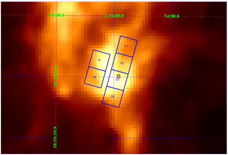
Figure 1: IRAS 100 $\mu$m image of MBM12, with the Chandra observation coordinates overlaid.

MBM12 is a relatively thin molecular cloud and so we must consider if it is optically thick to background X-rays even at the relatively soft energies of O VII ($\sim 0.57$ keV) and O VIII ($0.654$ keV). Assuming solar abundances, the cross sections at these energies are $9.4\times 10^{-22}$ cm^-2 per H atom and $6.7\times 10^{-22}$ cm^-2 per H atom, respectively (Balucinska-Church & McCammon, 1992). Measuring the column density over the face of the entire cloud is difficult. Absorption line measurements show the column density at one position; Luhman (2001) found that most stars in MBM12 have $A_{V}<2$, with background stars in the range $A_{V}=3-8$. Converting this to an equivalent hydrogen column density via N${}_{\rm H}/A_{V}=1.9\times 10^{21}$ cm^-2 mag^-1 (Allen, 1999) gives N${}_{\rm H}<3.8\times 10^{21}$ cm^-2 for much of the cloud, with a maximum value in the range N${}_{\rm H}=6-15\times 10^{21}$ cm^-2. SMV93 also measured the column density by cross-correlating the ROSAT 3/4 keV and IRAS 100$\mu$m flux, and derived a value of N${}_{\rm H}/F(100\mu m)=1.3^{+1.1}_{-0.1}\times 10^{20}$ cm${}^{-2}/$(MJy sr^-1). For these observations, the central ACIS-S3 detector was positioned on the brightest infrared position of MBM12, where $F(100\mu m)=30-35$ MJy sr^-1, so using the SMV93 ratio, N${}_{\rm H}=3.6-8.4\times 10^{21}$ cm^-2. Since we are observing in the direction of the densest part of MBM12, we believe N${}_{\rm H}=4\times 10^{21}$ cm^-2 is a conservative value. The opacity of MBM12 to background line emission is then $\tau$(O VII) = 3.76 and $\tau$(O VIII)= 2.68, and any distant emission will be reduced by 98% at O VII and 93% at O VIII. Only an extremely bright background source could affect our results, and this is unlikely. The ROSAT PSPC had a large $2^{\circ}$ field of view, and although SMV93 found some 3/4 keV emission off-cloud, it was only $\sim 3.3\times$ brighter than their $2\sigma$ upper limit for the 3/4 keV towards the cloud.

3.1 Data processing

The data reduction process was somewhat unusual, since emission from the LB completely fills the field of view, and the features of interest are extremely weak. Our original plan was to use the front-illuminated (FI) CCDs to measure the individual lines, and the back-illuminated (BI) CCDs (which have more effective area but lower resolution and higher background) to confirm the result. Based on the Gendreau et al. (1995) measurement of the soft X-ray background, we expected pre-launch to obtain at most $\sim 0.004$ counts/s from O VII and $\sim 0.001$ counts/s from O VIII lines from both the 4 (FI) ACIS-I CCDs and the (BI) ACIS S3 CCD. However, after the proton damage to the FI CCDs early in the mission, the highly row-dependent response of the FI CCDs means that these lines would be very difficult to extract robustly. Therefore, we focused on data from the BI CCD ACIS-S3.

We used CIAO 3.1 tools to process the observations, along with CALDB 2.27. Our result depends crucially on the background measurement, which must be done indirectly since the source fills the field of view. The two most important steps are removing flares and point sources. We followed a procedure similar to that described in Markevitch et al. (2003), although as the data were taken in FAINT mode, VFAINT filtering was not possible. For the purposes of source-finding only, we merged the two observations using the align_evt routine. We then ran celldetect, requiring $S/N>3$, which found 16 sources (including the well-known source XY Ari). We excluded all these sources, using circles of $15^{\prime\prime}$ radius (except XY Ari, where we used a $30^{\prime\prime}$ radius circle). This procedure eliminated $15\%$ of all events, with XY Ari alone accounting for $11\%$, and removed $5.0\%$ of the area leaving a total field of view of 67 arcmin². We then made a lightcurve of the ACIS-S3 events between 2.5-7 keV for each observation, as shown in Figure 2. We constructed a histogram of the observed rates and fit it with a Gaussian, representing the quiescent rate, plus a constant to roughly model the flares. We obtained good fits in both cases which showed that the quiescent level in the first observation was 0.22 cts/s while in the second it was 0.16 cts/s. The quiescent rate in the first observation is significantly above those shown in Markevitch et al. (2003), which ranged from 0.1-0.16 cts/s. These fluctuations in the background counting rate are likely due to protons which are trapped in the Earth’s radiation belts or directly from Solar flares.

Figure 2: (a) Lightcurve from the the first MBM12 observation between 2.5-7 keV, with a dashed line showing our best-fit quiescent rate of 0.22 cts/s. (b) Same, from the second observation, with a quiescent rate of 0.16 cts/s.

Following Markevitch et al. (2003), we removed all times when the count rate was not within 20% of the average rate for the second observation. The maximum allowed rate is therefore 0.192 cts/s, which limits the first observation to $2.2$ ksec of “good time,” too little data to be useful. This exclusion was not capricious. Although the first MBM12 observation was $\sim 40\%$ brighter than the average background rate for ACIS-S3, we expended substantial effort attempting to model it. All our attempts required adding what amounted to arbitrary terms at the same energies as our emission lines, so no conclusive results were possible. Therefore, we reluctantly excluded it from the remaining analysis. After filtering the second observation, we were left with 38.2 ksec of usable data.

To cross-check these results, we followed Markevitch et al. (2003) and compared the total counts in selected energy bands to the total counts seen with PHA values between 2500 and 3000. PHA values in this range correspond to energies above 10 keV, which are outside Chandra’s range and thus effectively measures the “particle background” rate. Table 1 shows the results for our MBM12 observations and one of our background datasets, ObsID 62850 (see §3.2). In Table 1 we show the results from the filtered Obi1 data as well as the 2.2 ksec of “good” data from Obi0 as well as values from all of Obi0. Ratios of the number of events in these bands to the number of events with PHA values between 2500 and 3000 are given as well. The unfiltered Obi0 data show very high ratios, suggesting contamination from some source besides the normal particle background. Conversely, the Obi1 observations of MBM12 show slightly higher ratios compared to the ObsID 62850 ratios, consistent with a weak source such as the diffuse X-ray background. The ratios seen for ObsID 62850 are similar to the average values observed by Markevitch et al. (2003) for the EHM observations.

Table 1: Total counts and ratios in selected bands

Band	ObsID 62850		MBM12 Obi1		“good” Obi0		“all” Obi0
	Counts	Ratio	Counts	Ratio	Counts	Ratio	Counts	Ratio
PHA (2500-3000)	36197	1.000	21735	1.000	1407	1.000	75925	1.000
0.5-2.0 keV	4762	0.132	4015	0.185	314	0.223	46387	0.611
2.0-7.0 keV	8545	0.236	7492	0.344	513	0.365	63693	0.839
5.0-10.0 keV	22742	0.628	14877	0.684	978	0.695	96311	1.269

3.2 Background

Since the LB fills the field of view in all normal Chandra observations, determining the true background is non-trivial. There are three types of Chandra observations which contain only instrumental or near-Earth background: the Dark Moon observation described in Markevitch et al. (2003), the Event Histogram Mode (EHM) data taken by ACIS during HRC-I observations and also described in Markevitch et al. (2003), and the ’stowed ACIS’ observations first described in Wargelin et al. (2004). These latter observations (to date, ObsID 4286, 62846, 62848, and 62850) were done with ACIS clocking the CCDs in “Timed Exposure” mode and reporting event data in the VFAINT telemetry format, and with ACIS in a ’stowed’ position at which ACIS receives negligible flux from the telescope and the on-board calibration source. We used data from ObsIDs 62848, 62848, and 62850 as our background datasets. Together these datasets represent 144 ksec of observations, although they were treated independently in our fits. ObsID 4286 is less than 10 ksec and was not used. Between our observations and the last of these observations (in December 2003) there was little change in the overall background rate.

We fit the MBM12 data from Obi1 simultaneously with stowed ACIS data using both a foreground and background model and Sherpa’s CSTAT statistic. The fits were restricted to the range 0.4 - 6 keV, since above 6 keV the background appears to rise due to the near-constant cosmic ray background combined with the falling mirror response, while below 0.4 keV the background rises and falls in a highly variable fashion. Our foreground model consisted of two unabsorbed delta functions for the O VII and O VIII lines, plus an absorbed power law and thermal component to represent the cosmic X-ray background and the distant hot Galactic component. We did not include a thermal component with $T\sim 10^{6}$ K to represent the LB emission, as nearly all of that emission would be below 0.4 keV, except for the oxygen lines. The absorption was allowed to vary between $N_{\rm H}$= $3.6-8.4\times 10^{21}$ cm² for both components; the best-fit value was $6\times 10^{21}$ cm² although our results were not particularly sensitive to this value. We used the values from Lumb et al. (2002) for the power-law component ($\Gamma=1.42\pm 0.03$, normalized to $8.44_{-0.23}^{+2.55}$ photons cm^-2s^-1keV^-1 at 1 keV), as well as for the temperature of the thermal component ($0.2\pm 0.01$ keV). The normalization on the thermal component was allowed to vary, since significant variation has been seen for this absorbed hot gas (Kuntz & Snowden, 2000). The O VIII Ly$\alpha$ line position was set at 0.654 keV. However, since the O VII emission is from a triplet of lines whose dominant member is unknown, we allowed the centroid of the line complex to float within a range of O VII line positions between the forbidden line at 0.561 keV and the resonance line at 0.574 keV. We found that the sharp rise seen below 0.5 keV in both the source and background could be fit using a low-energy Lorentzian, and also included delta functions at 1.78 keV (Si-K) and 2.15 keV (Au-M) to fit the particle-induced fluorescence seen at these energies. Finally, the particle-induced continuum background was modeled as a line with slope and offset, which was not folded through the instrumental response.

4 Results

Since we used the standard model of the diffuse X-ray background, we were not surprised to find a good fit to the data. The source model had only three significant parameters: the O VII and O VIII line fluxes, and the normalization on the absorbed Galactic thermal component. The total absorbed flux from this last component was only $F_{X}$(0.4-6 keV) = 0.066 photons cm^-2s^-1sr^-1, significantly less flux than from either of the two oxygen lines. Our results for the line emission are shown in Figure 3 and Table 2. Table 2 also lists O VII and O VIII fluxes measured at high Galactic latitude with ASCA (Gendreau et al., 1995) and the XQC (McCammon et al., 2002). In addition, line fluxes due to heliospheric charge exchange (Snowden, Collier & Kuntz, 2004, labeled SCK04) and geocoronal charge exchange (Wargelin et al., 2004, labeled “Dark Moon”) (see §5.1) are listed, along with the $2\sigma$ upper limits from the ROSAT observations of MBM12 (SMV93). The listed errors are $1\sigma$, except for the Wargelin et al. (2004) data where the 90% likelihood range is shown. The SMV93 limits assume all the emission is from that one line, since ROSAT could not resolve O VII from O VIII. When we allowed the O VII line to float between the forbidden and resonance line energies, we found that any value would lead to acceptable fits. The statistics and CCD resolution could not distinguish between either the low or high energy end, so our results are shown for an assumed “average” line position of 0.57 keV. Our best-fit O VII flux is consistent with the high-latitude Gendreau et al. (1995) results. However, the O VIII emission is significantly larger than the results of Gendreau et al. (1995) or McCammon et al. (2002). The strength of the O VIII is not strongly dependent on the details of background subtraction, since it is far from the rapidly rising background found at low energies on ACIS-S3. We conclude that this measurement is correct, but contaminated with Solar system emission from charge exchange. Other measurements in Table 2 show that charge exchange can easily swamp any LB emission. For example, the Wargelin et al. (2004) “bright” results from the dark Moon (from their Table 7) are significantly larger than either our results or those of Gendreau et al. (1995), and the same is true of the SCK04 results.

Table 2: Oxygen line emission (in LU)

Ion	This work	ASCA	XQC	SCK04	Dark Moon	SMV93
O VII	$1.79\pm 0.55$	$2.3\pm 0.3$	$4.8\pm 0.8$	$7.39\pm 0.79$	6.5-13.6	$<7.1$
O VIII	$2.34\pm 0.36$	$0.6\pm 0.15$	$1.6\pm 0.4$	$6.54\pm 0.34$	2.7-6.1	$<3.6$

Figure 3: [Top Left] Best-fit spectrum for MBM12 observation [Bottom Left] Best-fit background spectrum from ObsID 62850; note the fluorescence lines at 1.78 keV and 2.15. [Top Right] Best-fit spectrum from MBM12 between 0.4-1 keV, showing the strength of the oxygen lines. [Bottom Right] Same showing the background fit.

5 Discussion

Our original goal was to determine the age of the LB by measuring the ratio of the O VII and O VIII emission lines. In equilibrium, the O VIII emission would be negligible. A number of non-equilibrium models, however, predict detectable O VIII. Smith & Cox (2001) considered a range of models involving a series of supernova explosions. If the LB is still evolving 3-7 Myr after the last explosion, their Figure 13b suggests that the O VIII would still be detectable relative to the O VII emission. Alternatively, Breitschwerdt & Schmutzler (1994); Breitschwerdt (2001) would also imply a detectable amount of O VIII emission (see §5.3). Solar flares, the variable response of the ACIS-I, and complicated background of the ACIS-S3 CCD have proved significant but not insurmountable obstacles. However, the strong O VIII line is a much larger problem, since it is significantly larger than has been measured at high latitudes which include both the LB and Galactic halo emission. As stated above, it seems likely that our results have been contaminated by charge exchange with the solar wind.

5.1 Charge Exchange

Charge exchange, as first noted by Cox (1998), is a serious complication for diffuse soft X-ray background studies. Charge exchange creates X-rays when electrons jump from neutral material (usually hydrogen or helium atoms) to excited levels of highly ionized atoms. Charge exchange between neutral H and O⁺⁷, for example, can create O VII emission. The highly charged ions come from the solar wind and coronal mass ejections (CMEs). The neutral material can come from either the geocorona or the interstellar medium as it flows into the heliosphere; see Cravens (2000) for an overview of this mechanism. Cravens, Robertson & Snowden (2001) show that the so-called “Long Term Enhancements” (LTEs) observed during the ROSAT sky survey, which were apparent brightenings of the diffuse X-ray sky lasting days to weeks, can be explained by X-ray emission from charge exchange between the solar wind and either the geocorona or the interstellar medium, or both.

Wargelin et al. (2004) detected a strongly time-dependent O VII line along with weaker O VIII emission from Chandra observations of the dark Moon. The source of these X-rays is almost certainly charge exchange between solar wind ions and the geocorona. The time variability of the solar wind makes the time-dependence of the X-ray emission understandable. Detailed spectral models of charge exchange emission have been developed (e.g. Kharchenko & Dalgarno, 2001). Wargelin et al. (2004) used these calculations to model the O VII and O VIII geocoronal emission as a function of the solar wind oxygen ion flux (which can be estimated from ACE measurements). Their model estimates the surface brightness in each line as

$$L_{S}={{v_{c}n_{p}f_{O}y_{il}\sigma_{i}n_{n0}}\over{4\pi}}5R_{E}\big{(}{{10R_{E}}\over{r_{min}}}\big{)}^{2}$$ (1)

where $v_{c}$ is the solar wind velocity, $n_{p}$ the proton density, $f_{O}$ the relative abundance of oxygen, $y_{il}$ the line yield per charge exchange, $\sigma_{i}$ the charge exchange cross section, and $n_{n0}$ the neutral particle density at 10 Earth radii ($R_{E}$). $r_{min}$ is the geocentric distance to the edge of the magnetosphere or the spacecraft position, whichever is farther. Some of these parameters are measured by the ACE satellite. This model predicts that the O VIII/O VII ratio due solely to charge exchange is $1.36(n_{O^{+8}}/n_{O^{+7}})+0.14$, where $n_{I}$ is the density of ion I. This result uses values from Tables 5 and 6 of Wargelin et al. (2004) and including the O VII K$\beta$ line in the O VIII emissivity, since they would be blended. In a typical slow solar wind, $n_{O^{+8}}/n_{O^{+7}}\approx 0.35$, implying a ratio of 0.616 (SCK04). Unfortunately, ACE does not yet routinely provide measurements of $n_{O^{+8}}/n_{O^{+7}}$, as it does with $n_{O^{+7}}/n_{O^{+6}}$. During Obi1, $n_{O^{+7}}/n_{O^{+6}}$ was $\sim 0.7$, approximately midway between the average value for the slow solar wind ($\sim 0.3$) and the value of $\sim 1.4$ measured during the brightest dark Moon observations.

Going beyond the Earth-Moon system, the time-variable effects of charge exchange in the broader heliosphere were measured by SCK04. They used a series of four XMM-Newton observations of the Hubble Deep Field North (a high-latitude patch of sky devoid of bright X-ray sources) to measure O VII and O VIII emission and correlated their results with solar wind observations from ACE. They found that three out of four observations (as well as part of the fourth) agreed with the standard diffuse X-ray background model, and that during these times the proton flux and $n_{O^{+7}}$/$n_{O^{+6}}$ ratios in the solar wind were $1.5-3.2\times 10^{8}$ cm^-2s^-1 and $0.15-0.46$, respectively. However, part of the fourth observation showed substantially brighter O VII and O VIII, as well as sharp increases in both the proton flux (to $8.0\times 10^{8}$ cm^-2s^-1) and the $n_{O^{+7}}$/$n_{O^{+6}}$ ratio (to 0.99). Their measured heliospheric surface brightnesses are given in Table 2.

Our viewing geometry for MBM12 during Obi1 is such that we would expect an effect due to charge exchange, especially for O VII. The heliospheric “downstream” direction, with respect to the Sun’s motion through the Local Cloud is centered around ecliptic coordinates $74.5^{\circ},-6^{\circ}$ (Lallement and Bertin, 1992), which corresponds to December 5 for the Earth’s orbital position. MBM12 ($47.6^{\circ},+3^{\circ}$ in ecliptic coordinates) is not far from this direction, so when Obi1 was done on August 17 it should have been viewing a sparse column of neutral heliospheric gas–mostly He, since the H would be largely ionized as it flowed by the Sun. From Table 9 of Wargelin et al. (2004), we therefore expect, for a typical slow solar wind, a total ROSAT surface brightness of $\sim 470$ cts s^-1sr^-1. The geocoronal component should be roughly $\sim 1/4$th of this, as the viewing direction is (roughly) through the flank of the magnetopause, again from Table 9 of and Figure 7 of Wargelin et al. (2004). We therefore expect the total surface brightnesses will be $\sim 5\times$ the geocoronal model values in Table 8 of Wargelin et al. (2004), or 1.4 and 0.56 ph cm^-2s^-1sr^-1 for O VII and O VIII, respectively. Given the uncertainties, and the expectation that charge exchange emission does not account for the entire soft X-ray background observed by ROSAT (but see Lallement, 2004), the O VII prediction matches our result well, but the O VIII is still anomalously high for a typical slow solar wind alone.

However, in addition to the solar wind, it should be noted that there were a number of halo CME events during 2000 July. These would have the effect of mixing into the Earth’s side of the interplanetary medium some CME plasma that may well have a substantially higher ionization state. These vary from event to event, and there are only a few events which are suitable for study both in the near sun environment with SOHO and in situ with a solar wind ion charge state spectrometer.

As an example, one such event was observed in 2002 November and December (Poletto et al., 2004). The UVCS data measured remotely by the SOHO observatory at 1.7 solar radii above the solar limb show lines of Fe XVIII, and the SWICS data measured in situ by Ulysses also show high ions of iron (Fe⁺¹⁶ being prominent). This leads these authors to conclude that, for this CME event, the ionization state is characteristic of a ”freezing in” temperature in excess of 6 MK. At such temperatures, oxygen is fully ionized.

Cravens (2000) argues that solar wind charge exchange with the neutral interstellar medium (ISM) mostly occurs at distances of a few AU from the sun because of the depletion of neutral gas near the Sun. Since 100 km s^-1 translates to about 1.7 AU per month, and CME fronts range from about 20 to over 2000 km s^-1 (Webb, 2002), we are not concerned with a single event but an average over the week or two prior to the observation.

We therefore conclude that the large O VIII/O VII ratio we observe could be expected from the charge exchange of CME plasma with the neutral ISM, but that the details are sufficiently complex (and the data sufficiently sparse) that prediction of this ratio is difficult to impossible. We can say, however, that the observed O VII and O VIII provides a (weak) upper limit to the emission from the LB.

5.2 Collisional Models

What do these observations imply if the observed line emission is due to electron/ion interactions rather than charge exchange? In this case it is relatively easy to calculate the expected contribution from each atomic process. O VII emission from any of the triplet of lines is created by direct excitation (where we include cascades from excitation to higher levels), electron recombination onto O⁺⁷, or inner-shell ionization of O⁺⁵. O VIII lines come from direct excitation or recombination from bare oxygen ions; K-shell ionization of O⁺⁶ does not have a large cross section for emitting O VIII. If the plasma is at or near ionization equilibrium we can ignore blending from satellite lines or other emission lines in the region of interest as they should contribute only a small fraction of the total emission; we consider the far-from-equilibrium case in §5.3. For example, at CCD resolution the O VII $1s3l\rightarrow 1s^{2}$ line will blend with the O VIII Ly$\alpha$ line. However, it contributes at most 6% of the flux of the O VIII Ly$\alpha$ line and so can be ignored to a first approximation.

With these assumptions, the observed line surface brightness (in LU) along a particular line of sight can be written as

$$L_{S}(\hbox{{O~{}VII}}) = {{1}\over{4\pi}}\int dR{{n_{e}^{2}(r)}\over{1.2}}[n_{+5}(r)\Lambda_{\hbox{\small{O~{}VII}}}^{IS}(T)+$$ (2)

$$n_{+6}(r)\Lambda_{\hbox{\small{O~{}VII}}}^{DE}(T)+n_{+7}(r)\Lambda_{\hbox{\small{O~{}VII}}}^{RC}(T)]$$

$$L_{S}(\hbox{\small{O~{}VIII}}) = {{1}\over{4\pi}}\int dR{{n_{e}^{2}(r)}\over{1.2}}[n_{+7}(r)\Lambda_{\hbox{\small{O~{}VIII}}}^{DE}(T)+$$ (3)

$$n_{+8}(r)\Lambda_{\hbox{\small{O~{}VIII}}}^{RC}(T)]$$

where L_S is in LU, $n_{e}(r)$ is the electron density at distance $r$, $n_{+n}(r)$ is the ion density of O⁺ⁿ at $r$. We also assume that the hydrogen and helium are fully ionized, so $n_{e}\approx 1.2n_{H}$. $\Lambda_{I}^{IS}(T)$, $\Lambda_{I}^{DE}(T)$, $\Lambda_{I}^{RC}(T)$ are the rate coefficients (in cm³ s^-1) for creating an emission line via inner-shell, direct excitation, or recombination for ion I, and are plotted in Figure 4.

Figure 4: $\Lambda$ curves as a function of electron temperature, using APEC and data from ATOMDB 1.3.1. The total emission from each process is $n_{e}n_{I}\Lambda.$

Since four different ions may be involved in creating O VII and O VIII emission lines, we cannot uniquely solve for the density, temperature, and ionization state of the system. However, we can easily show that these line fluxes are not commensurate with an equilibrium plasma. The O VIII flux provides the strongest limit, as this line is not expected in an equilibrium model for the LB. Figure 4 shows that the direct excitation rate for this line rises rapidly with temperature, so a higher temperature will produce more O VIII. Based on the Kuntz & Snowden (2000) survey of LB results (see their Table 1), we assume that the allowed electron temperature in the LB is $<2\times 10^{6}$ K; in equilibrium at this temperature $n_{O^{+6}}$/$n_{O^{+7}}>1$. Figure 4 clearly shows that the direct excitation rate for O VII is more than triple the rate for O VIII excitation, which would predict O VII/O VIII $>3$, in strong contrast to our result. Therefore, either the O VIII line emission is not coming from the LB, or the plasma is recombining, with significantly more O⁺⁷ or O⁺⁸ ions than O⁺⁶ ions. We consider some aspects of this possibility below.

5.3 Recombining Plasma Models

Breitschwerdt & Schmutzler (1994) proposed a radical new model for the LB suggesting that it was not in fact “hot” but rather the X-ray emission was created by recombination of highly-ionized atoms with cool ($10^{4}-3\times 10^{5}$ K) electrons. Their model assumes the LB was a pre-existing cavity, probably formed by a earlier supernova explosions and possibly associated with the Sco-Cen superbubble. Then inside this cavity a few million years ago a massive star inside a dense cloud exploded. After the SN shock heated and ionized the entire cloud, the resulting hot ions expanded into the low-density cavity and cooled adiabatically. This model was partially inspired by the relatively high average density of 0.024 cm^-3 measured from a nearby (130 pc distant) pulsar’s dispersion measure(Reynolds, 1990). If this density is representative of the LB as a whole, a $\sim 10^{6}$ K plasma would create far more soft X-rays than are observed. Breitschwerdt & Schmutzler (1994) showed that a low-temperature, high-ionization state plasma with this density could generate the observed 1/4 keV X-ray emission. Later papers (Breitschwerdt et al., 1996; Breitschwerdt, 2001) have described the model in more detail and made predictions of the flux in various bandpasses. This model also naturally explained the existence of the “Local Fluff,” neutral H I clouds (e.g. Bochkarev, 1987; Frisch, 1995) which are hard to understand in the context of “hot” bubble models.

Although more complicated than the equilibrium isothermal LB model, a strength of this model is that it does not require a particular fine-tuning or a complicated mix of hydrodynamic and plasma models. As noted by Breitschwerdt (2001), only some basic input parameters – cavity radius R, electron density $n_{e}$, electron temperature $T_{e}$, and evolution time $t$ – are needed and a fairly wide range of these values matched the available data at the time.

However, FUSE observations (Shelton, 2003) put a surprisingly low $2\sigma$ upper limit on the O VI $\lambda\lambda$1032,1038 emission from the LB of 500 and 530 LU, respectively, and 800 LU for both lines combined. Shelton (2003) noted that this result alone strongly constrains any recombining plasma model and when combined with other discrepancies in the C III emission and the N(O VI) column density “practically eliminate[s] this class of models.” However, this argument rests on discrepancies in two unrelated ions, O VI and C III, leaving open the possibility that these issues could be finessed with the correctly-tuned input parameters. Recombining plasma models are still being invoked in recent papers (e.g. Freyberg, Breitschwerdt & Alves, 2004; Hurwitz, Sasseen & Sirk, 2004). The O VI upper limits are quite stringent, however, and combining them with our measurements allows a rigorous test of the model using all relevant oxygen ions as they recombine from fully stripped O⁺⁸ to O⁺⁵ and beyond. Any acceptable recombining plasma model would have to match the upper limits found for each ion’s emission lines, while also emitting at least some of the observed 1/4 keV band X-rays.

Interestingly, in the case of a purely recombining plasma, the ionization state of the plasma at any point in its evolution can be calculated analytically. If ionization can be ignored, the population of any ion state can be written as:

$${{dp^{i}}\over{dt}}=-R_{i}n_{e}p^{i}+R_{i+1}n_{e}p^{i+1}$$ (4)

where $p^{i}$ is the population of the ion with $i$ electrons and $R_{i}$ is the recombination rate (in cm³ s^-1) from the $i$th ion state to the $i+1$ state. In the case of the fully-stripped ion ($p^{0}$), the second term in Eq. (4) is zero as there is no higher ion. Equation (4) then leads to a linked series of first order differential equations that can be easily solved. Assuming that initially the population is fully stripped ($p^{0}(0)\equiv 1$), the population of any ion can be written as:

$$p^{i}=\sum_{j=0}^{i-1}\Big{[}{{R_{i-1}f_{j}^{i-1}}\over{R_{i}-R_{j}}}(\exp(-R_{j}n_{e}t)-\exp(-R_{i}n_{e}t))\Big{]}$$ (5)

where $f_{j}^{i}$ equals 1 when $i=j=0$ and is otherwise defined by the recursion relation:

$$f_{j}^{i}=\cases{{{R_{i-1}f_{j}^{i-1}}\over{R_{i}-R_{j}}}&if $j<i$\cr-\sum_{j=0}^{i-1}{{R_{i-1}f_{j}^{i-1}}\over{R_{i}-R_{j}}}&if $j=i$\cr}$$ (6)

To calculate $R_{i}$ we used radiative recombination rates from Verner & Ferland (1996) and dielectronic rates from Romanik (1988, 1996). Combining this with Figure 4 we can calculate the predicted O VIII Ly$\alpha$ and O VII triplet flux due to recombination for any temperature and density. We calculated the O VI flux from electron collisions (recombination from O⁺⁶ was negligible) using the collision strengths from Griffin, Badnell, & Pindzola (2000).

However, the upper limits on the O VIII, O VII, and O VI emission and the N(O VI) column density were not sufficient, as a sufficiently low density would always be allowed (see Figure 5[Lower Right]). The recombining ion model, however, was initially developed with a relatively high density in mind and tested against the observed 1/4 keV band emission. We have developed an approximate but robust model of the X-ray spectrum from a recombining plasma to compare to the ROSAT R12 band emission. This model considered only emission from dielectronic and radiative recombination, omitting direct excitation. In a plasma with low electron temperature, the radiative recombination continuum appears as a nearly line-like (width $\sim kT$) feature at the binding energy of the recombined level. We therefore assumed that each radiative recombination led to a photon at the binding energy of the ion; this ignores cascades which would modify somewhat the exact distribution of the photons but is reasonably accurate for our purposes. The dielectronic satellite lines were calculated using data from Romanik (1996, 1988). We then folded the resulting spectrum between 50-1000 eV through the ROSAT R12 band response to calculate the expected emission in this band.

For the O VII and O VIII limits we used the $2\sigma$ upper limits from the MBM12 observation, despite our strong suspicion (based on the ACE data and the odd ratio of the two lines) that these are already contaminated by charge exchange. In addition, in the case of O VIII our $2\sigma$ upper limit is larger than the value observed by the XQC (McCammon et al., 2002) over a 1 sr field of view, which necessarily includes both LB and more distant emission. Therefore, we feel this is a very conservative upper limit to the local contribution from O VII and O VIII

Defining an “upper limit” to the column density of O VI in the LB is difficult, and so we attempted to determine a reasonable value by indirect methods. Shelton & Cox (1994) found through a statistical analysis that the most likely value for N(O VI) in the LB was $1.6\times 10^{13}$ cm^-2. The Copernicus data this was based on Jenkins (1978) also shows that no O or B star within 250 pc has a column density greater than this value. In addition, FUSE results towards 25 nearby white dwarfs (Oegerle et al., 2004) show at most $1.7\times 10^{13}$ cm^-2, with an average value of $\sim 7\times 10^{12}$ cm^-2. We therefore chose N(O VI) $<1.7\times 10^{13}$ cm^-2 as our upper limit to the column density of O VI through the LB.

We wanted to choose a very conservative value for the minimum R12 band emission from the LB required by the model. Breitschwerdt & Schmutzler (1994) assumed some of the observed soft X-ray emission came from distant superbubbles, since ROSAT had recently seen clouds in absorption. Nonetheless, they also required some local emission, although the required amount was somewhat uncertain. Since then, Kuntz, Snowden & Verter (1997) studied the foreground X-ray emission by analyzing the shadows seen by ROSAT towards nearby molecular clouds. They measured the foreground R12 emission seen towards 9 clouds, finding a range of 3790 - 6190 counts s^-1 sr^-1. This was followed by the exhaustive study of X-ray shadows by Snowden et al. (2000), who examined 378 clouds seen with ROSAT. Their results showed substantial variation from position to position, with a mean and standard deviation of 5810$\pm$1960 counts s^-1 sr^-1. Based on these results, we decided to require at least 910 counts s^-1 sr^-1 in the R12 band, far below the value found by Kuntz, Snowden & Verter (1997) and $2.5\sigma$ below the Snowden et al. (2000) mean value.

In Figure 5 we show the predicted O VIII, O VII, and O VI emission, the O VI column density, the R12 emission for two recombining plasma models, and the maximum allowed electron density based solely on the oxygen ion upper limits for both models. The oxygen, neon, and argon abundances were taken from Asplund et al. (2004), with all other abundances from Anders & Grevesse (1989). The plots are shown as functions of the fluence ($\equiv n_{e}t$), a convenient variable as all the rates are proportional to the electron density. The thick curves show the results for the model described in Breitschwerdt (2001), with a cavity radius of 114 pc, an electron density of $0.024$ cm^-3, and an electron temperature of $3\times 10^{5}$ K. Note how the R12 emission matches the observations over a wide range of fluences, suggesting that our 1/4 keV emission model agrees with that used in Breitschwerdt (2001). Whenever the R12 emission reaches and exceeds the lower limit in this model, though, the O VI emission exceeds its upper limit. The thin curves show a second model, with the same radius, an electron density of 0.01 cm^-3, and an electron temperature of $2\times 10^{4}$ K. In this case there is a small region with fluence $\sim 10^{10}$ cm^-3s where the R12 and O VI emission pass their lower and upper limits, respectively. However, in this range the predicted O VII and O VIII substantially exceed the upper limits towards MBM12. At later fluences the predicted O VII and O VIII emission drops but the N(O VI) column density exceeds the observed value. In sum, there is no point which simultaneously meets all the upper and lower limits.

The R12 emission calculation is necessary, since it provides the only lower limit, but it is also quite complex to calculate and it is useful to consider what can be derived purely from the simpler oxygen ions. Figure 5[Bottom Right] plots the limit on the electron density available purely from the oxygen emission and absorption upper limits. For example, the O VIII emission is given by

$${\hbox{{O~{}VIII}}}=n_{e}n_{+8}{R\over{4\pi}}\Lambda_{\hbox{\small{O~{}VIII}}}^{RC}(T)$$ (7)

which can easily be converted into an upper limit on the electron density since the remaining terms are determined by recombining ion model. As can be seen in the model, the limits from the Oxygen ions alone require the electron density to be below the assumed density until very late times or fluences.

Figure 5: [Top Left] The O VIII Ly$\alpha$, O VII triplet, and O VI doublet emission and observed upper limits for two different models as a function of fluence. Thick curves show a model with $R=114$ pc, $n_{e}=0.024$ cm^-3, and $T_{e}=3\times 10^{5}$ K, thin lines are for a model with $R=114$ pc, $n_{e}=0.01$ cm^-3, and $T_{e}=2\times 10^{4}$ K [Top Right] The O VI column density in the LB for the same models, along with the observed upper limit from the LB. [Bottom Left] The ROSAT R12 emission from both models, with a line showing our estimated lower limit. [Bottom Right] The maximum allowed electron density for a 114 pc bubble in either model, based only on the O VIII, O VII, and O VI limits. The effects of each Oxygen ion’s limit are visible. Except at large fluences (when the R12 emission is negligible), the maximum allowed density is less than the assumed model density, showing why these models are excluded.

We have examined a wide range of input parameters for the recombining plasma model. We considered electron densities up to 0.03 cm^-3, electron temperatures in the range $10^{4}-5\times 10^{5}$ K and all cavity radii between 30-300 pc and followed each set of values for $10^{7}$ years, the maximum plausible lifetime of the LB. Although the results vary substantially with the input parameters, as shown in Figure 5, none of our input parameters lead to predicted values that can simultaneously match these observational limits. In essence, the R12 lower limit requires a minimum density of highly ionized ions while the tight observational limits on O VI, O VII, and O VIII simultaneously limits the density of these ions. We can with confidence dispose of at least the static recombining plasma model.

6 Conclusions

We have observed the nearby molecular cloud MBM12 with Chandra, and measured the foreground O VII and O VIII surface brightness towards the cloud, which should absorb any distant emission. Our observed values are higher than expected, and it appears likely, based on the ACE satellite data, that charge exchange in the heliosphere or geocorona has contaminated our results. We measure a unexpectedly low ratio of O VII/O VIII $=0.76\pm 0.26$, which is hard to understand in the context of other measurements or most LB models. In addition, circumstantial evidence also suggests that our results could be contaminated by charge exchange.

Despite this limitation, we are able to combine our upper limits with results from FUSE on O VI emission and absorption and the 1/4 keV ROSAT R12 emission to reject the constant temperature recombining plasma model originally proposed by Breitschwerdt & Schmutzler (1994) over a wide range of input parameters. Since the sole moderate-resolution spectrum of the LB taken by DXS showed that the constant temperature equilibrium model could also be rejected (Sanders et al., 2001), this result implies that more complex models of the soft X-ray emission from the LB are required.

A number of more complex models have been proposed, however (e.g. Smith & Cox, 2001; de Avillez & Breitschwerdt, 2003), and selecting amongst the various possibilities will require high resolution observations. If for example we could resolve the O VII triplet we would be able to determine if the plasma is ionizing, recombining, or both in different regions. Although Astro-E2 will have the necessary resolution, its effective area-solid angle product is only $\sim 330$ cm² arcmin², compared to $\sim 20,000$ cm² arcmin² for ACIS-S3. Constellation-X, however, will be a powerful instrument for understanding the recent history of our local environment.

We are grateful to Don Cox, Mike Juda, John Raymond, Robin Shelton, Steve Snowden, and Shanil Virani for helpful discussions. This work was supported by the Chandra X-ray Science Center (NASA contract NAS8-39073) and NASA Chandra observation grant GO0-1097X.

References

- Acton & Brown (1978) Acton, L. W. & Brown, W. A. 1978, ApJ, 225, 1065
- Allen (1999) “Allen’s Astrophysical Quantities (4th ed)”, 1999, ed. D. P. Cox, (AIP Press: New York), p. 197
- Anders & Grevesse (1989) Anders, E. & Grevesse, N. 1989, Geochimica et Cosmochimica Acta, 53, 197
- Andersson et al. (2002) Andersson, B.-G., Idzi, R., Uomoto, A., Wannier, P. G., Chen, B., & Jorgensen, A. M. 2002, AJ, 124, 2164
- Asplund et al. (2004) Asplund, M., Grevesse, N., Sauval, A. J., Allende Prieto, C., & Kiselman, D. 2004, A&A, 417, 751
- Balucinska-Church & McCammon (1992) Balucinska-Church, M. & McCammon, D. 1992, ApJ, 400, 699
- Bochkarev (1987) Bochkarev, N. G. 1987, Ap&SS, 138, 229
- Bowyer, Field & Mack (1968) Bowyer, C. S., Field, G. B., & Mack, J. E. 1968, Nature, 217, 32