Discovery of magnetic fields in central stars of planetary nebulae

For the first time we have directly detected magnetic fields in central stars of planetary nebulae by means of spectro-polarimetry with FORS1 at the VLT. In all four objects of our sample we found kilogauss magnetic fields, in NGC 1360 and LSS 1362 with very high significance, while in EGB 5 and Abell 36 the existence of a magnetic field is probable but with less certainty. This discovery supports the hypothesis that the non-spherical symmetry of most planetary nebulae is caused by magnetic fields in AGB stars. Our high discovery rate demands mechanisms to prevent full conservation of magnetic flux during the transition to white dwarfs.

1 Introduction

The reason why more than 80% of the known planetary nebulae (PNe) are mostly bipolar and not spherically symmetric (Zuckerman & Aller 1986; Stanghellini et al. 1993) is barely understood. A popular explanation is the interacting stellar winds model (Kwok et al. 1978), where the fast ($v\approx 1000$ km/sec, mass loss $\approx 10^{-7}\mbox{\,$\rm M_{\odot}$}/$yr) wind from the central star of a PN encounters an older slow ($v\approx 10$ km/sec) wind from earlier phases with heavy mass loss ($\approx 10^{-5}\mbox{\,$\rm M_{\odot}$}$/yr). The visible PN is formed in the shock region between both winds; if the slow wind was not spherical, but densest in the equatorial plane, the nebula is bipolar. However, neither is this model indisputable, nor is the physical mechanism for the asymmetry of the slow wind clear. One possibility is the presence of a low-mass companion star which could exert a gravitational pull on the circumstellar envelope. Rapid rotation and binarity (e.g.  De Marco et al. 2004) may also cause asymmetries, but the most promising explanations involve magnetic fields. There is, however, no agreement about the detailed mechanism. A review on observational and theoretical studies of the shaping of planetary nebulae is given by Balick & Frank (2002).

It is possible that magnetic fields from the stellar surface are wrapped up by differential rotation so that the later post-AGB wind will be collimated into two lobes (García-Segura et al. 1999). Another scenario says that magnetic pressure at the stellar surface plays an important role driving the stellar wind on the AGB (Pascoli 1997).

The idea that magnetic fields are important has been supported by the detection of polarization in radio data of circumstellar envelopes of AGB stars: SiO (at a distance of 5-10 AU from the star), H₂O ($\approx 100$ AU), and OH (100-1000 AU) masers (Kemball & Diamond 1997; Szymczak & Cohen 1997; Vlemmings et al. 2002).

For H₂O masers Vlemmings et al. (2002) are convinced that the Zeeman interpretation is correct and that the magnetic field strength at the H₂O maser of the Mira variable U Her is about 1.5G. Depending on the topology of the magnetic field, the corresponding surface magnetic field is of the order of 100-1000 G.

The magnetic field may be either a fossil remnant from the progenitor on the main sequence (e.g. Ap stars), or can be generated by a dynamo at the interface between a rapidly rotating stellar core and a more slowly rotating envelope. Blackman et al. (2001) argue that some remnant field anchored in the core will survive even without a convection zone, although the convective envelope may not be removed completely. Thomas et al. (1995) have shown that white dwarfs which do have thin surface convection zones can support a near-surface dynamo. Since the field strength in their model is higher at higher luminosities this would particularly be true for central stars of PNe.

That some central stars must contain significant magnetic fields is also obvious from the fact that at least 10-30% of all white dwarfs have magnetic fields between $10^{3}$ and $10^{9}$ Gauss. Until now no magnetic fields have ever directly been detected in central stars of PNe.

We have observed a sample of four central stars of planetary nebulae with high signal-to-noise (circular) spectropolarimetry between 3500 and 5900 Å  with the FORS1 spectrograph of the VLT telescope. As was already demonstrated for bright white dwarfs (Aznar Cuadrado et al. 2004), the unprecedented light collecting power of the VLT offers the possibility to investigate the presence of magnetic fields on the kG level.

2 Observations and data reduction

The observations were obtained in service mode between November 2, 2003, and January 27, 2004, with the FORS1 spectrograph of the UT1 (“Antu”) telescope of the VLT, which is able to measure circular polarization with the help of a Wollaston prism and rotatable retarder plate mosaics in the parallel beam allowing linear and circular polarimetry and spectropolarimetry (Appenzeller et al. 1998). We used grism G600B, covering the spectral range 3400–5900  Å, and a 0.8$\arcsec$ wide slit, leading to a spectral resolution of 4.5 Å. The details of our observations are listed in Table 1. The four selected objects are bright ($V\leq 12\hbox{$.\!\!^{\rm m}$}5$) and their nebulae show clear indications for non-spherical symmetry. So that we obtained at least one good result for a star, we decided to spend four times as much observing time on the CPN of NGC 1360 then on the other three objects, for which only one observing block was performed. In order to reduce errors from changes in the sky transparency, atmospheric scintillation, and various instrumental effects the $\lambda/4$-retarder plate was rotated by $90^{\circ}$ after $n$ exposures (where $n$ is given in the last column of Table 1). The same number of exposures were then taken in this configuration.

2.1 Data reduction

Calibration frames (bias, flat-field and He+HgCd arc spectra) were taken during the day, following each nights observations. The data were reduced in the iraf environment using the following procedure. The bias level was subtracted from all frames and cosmic rays were removed. A nightly master flat field was then constructed from each night’s individual flat fields. After flat-field correction, the stellar spectra were extracted from each frame by summing up all CCD rows for the ordinary and extraordinary ($e$ and $o$) beams. Background sky light was averaged over 10 rows (giving a total of 20 rows) on either side of the object spectrum and subtracted. It is important to note that the automatic aperture and sky selection routine in iraf does not always use the user-defined values, so each spectrum was checked manually.

Wavelength calibration is particularly important for this kind of spectropolarimetric study, and special care was taken to ensure its accuracy. Failure to do so would lead to spurious polarization signals in every line. Calibration was done independently for the spectra of each beam and each position of the retarder plate (i.e. the $e$ and $o$ beams at $\pm 45^{\circ}$).

The referee suggested that spurious signals may be caused by using arc spectra taken at different waveplate angles, probably because the spectra are rebinned differently. To test this we examined two cases: when the dispersion correction was applied, all spectra were forced to exactly the same scale or they were simply corrected according to the dispersion function only. In these two cases the spectra were rebinned differently. When we determine the magnetic field strength, however, the results are the same within errors. This indicates that rebinning is not affecting our results. We have also examined the sky spectral lines at the edge of our spectra; these lines show no detectable polarisation, suggesting that any polarisation we measure is intrinsic to the star and not due to poor wavelength calibration. Finally we note that while instrumental polarisation dominates the Stokes V/I spectrum when considering only one waveplate angle, we are encouraged to see the polarisation profiles at the positions of the Balmer and He II lines. The wavelengths are accurate to typically $\sim$3 km s^-1 or $\sim$0.05 Å at H$\beta$. This is much lower than the spectral resolution.

Stokes $I$, or unpolarized, spectra were obtained simply by summing all spectra taken of an object in a single night. The Stokes $V/I$ spectra, describing the net circular polarization, were created by summing the exposures made at the same retarder plate position angle, and then applying the following equation

$$\frac{V}{I}=\frac{R-1}{R+1},\;\mathrm{with}\>R^{2}=\left(\frac{f_{o}}{f_{e}}\right)_{\alpha=+45}\times\left(\frac{f_{e}}{f_{o}}\right)_{\alpha=-45},$$ (1)

which is equivalent to formula 4.1 in the FORS 1+2 User Manual (Szeifert & Böhnhardt 2003). Here $\alpha$ indicates the nominal value of the position angle of the retarder-wave plate, and $f_{o}$ and $f_{e}$ are the fluxes on the detector from the $e$ and $o$ beams of the Wollaston prism, respectively. The resulting high-quality spectra are shown in Fig. 1, while Figs. 2$-$3 show the circular polarization ($V/I$) spectra.

Table 1: Details of VLT observations. The coordinates $\alpha$ and $\delta$ refer to epoch 2000.

Target	Alias	$\alpha$	$\delta$	$V$	HJD	$t_{\mathrm{exp}}$	n
				(mag)	(+2 452 900)	(s)
NGC 1360	CD–26 1340	03 33 14.7	$-$25 52 18	11$.\!\!^{\rm m}$2	46.782	104	6
					88.725	104	6
					89.549	104	6
					90.571	104	6
EGB 5	PN G211.9+22.6	08 11 12.8	+10 57 19	12$.\!\!^{\rm m}$5	88.854	331	3
LSS 1362	PN G273.6+06.1	09 52 44.5	$-$46 16 51	12$.\!\!^{\rm m}$5	89.796	331	3
Abell 36	PN G318.4+41.1	13 40 41.4	$-$19 52 55	11$.\!\!^{\rm m}$5	131.773	150	5

3 Determination of the magnetic field strenghs

For weak magnetic fields (i.e. below 10 kG) theoretical polarization spectra ($V/I$) can be obtained by using the weak-field approximation (e.g., Angel & Landstreet 1970; Landi degl’Innocenti & Landi degl’Innocenti 1973):

$$\frac{V}{I}=-g_{\rm eff}C_{z}\lambda^{2}\frac{1}{I}\frac{\partial I}{\partial\lambda}\langle\large B_{z}\large\rangle\;,$$ (2)

where $g_{\rm eff}$ is the effective Landé factor (which is unity for Balmer lines and for the hydrogenic He II lines; Casini & Landi degl’Innocenti 1994), $\lambda$ is the wavelength expressed in  Å, $\langle B_{z}\rangle$ is the mean longitudinal component of the magnetic field expressed in Gauss and the constant $C_{z}=e/(4\pi m_{e}c^{2})$ $(\simeq 4.67\times 10^{-13}\,{\rm G}^{-1}\,\mbox{\AA}^{-1})$. Since we do not have any information about the detailed field geometry we can only measure the mean longitudinal field over the stellar surface. The maximum field strength can be larger than this value.

Since both the hydrogen lines and the He II lines have an effective Landé factor of unity we do not expect blending to have a large influence. However, it is clear that the total effect of two separate spectral lines on the polarization is not the same as treating a blended line in the same way. With our method it is not possible to disentangle both effects. Test calculations using theoretical spectra for NGC 1360 have shown that the result when using blended Balmer and He II lines instead of a sum of non-blended lines (by switching hydrogen or helium, respectively, in the calculation of the theoretical spectrum) differ by only about 200 G.

Figure 1: Normalized spectra of our sample of central stars of planetary nebulae (from above displaced vertically: NGC 1360, EGB 5, LSS 1362, Abell 36)

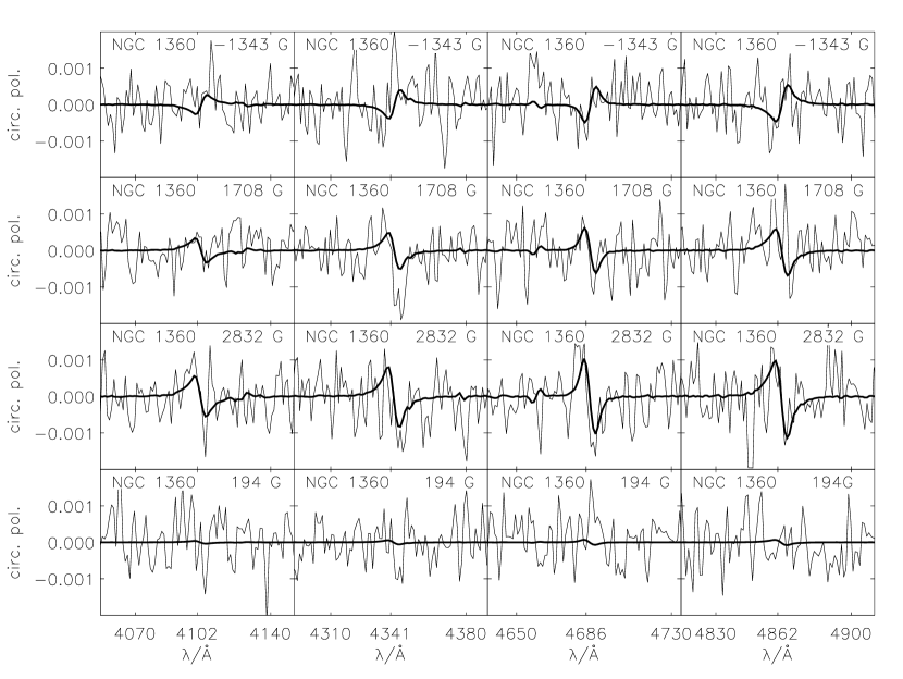
Figure 2: Circular polarization ($V/I$) in the four observation blocks of of the central star of NGC 1360 in the vicinity of the strong spectral lines H$\delta+$He II, H$\gamma+$He II, He II 4686, H$\beta+$He II compared to the prediction by the low-field approximation (Eq. 2) using a longitudinal magnetic field of $-1343$ G, $1708$ G, $2832$ G, and $194$ G, respectively

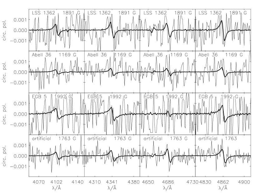
Figure 3: Circular polarization ($V/I$) observed in the central stars of LSS 1362, Abell 36, and EGB 5 in the vicinity of the strong spectral lines H$\delta+$He II, H$\gamma+$He II, He II 4686, H$\beta+$He II compared to the prediction by the low-field approximation (Eq. 2) using a longitudinal magnetic field of $1891$ G, $1169$ G, and $1992$ G. In the lower level we show an example for a fit to one of the artificial spectra with a noise level of 0.0005 and an assumed magnetic field of 1500 G. The fit results in $B=1763$ G

Figure 4: Result of the fits with simulated data having the same noise level as the observations of NGC 1360 for input magnetic fields between 0 and 3000 G, in steps of 500 G. From center line to outside: mean fit result, 1$\sigma$ error range, 99% confidence level, and smallest and largest fit result during the 1000 simulations which were performed for each predescribed magnetic field.

The longitudinal component of the magnetic field for each measurement was determined by comparing the observed circular polarization for an interval of $\pm 20$  Å around the four strongest absorption lines H$\beta+$He II, He II 4686, H$\gamma+$He II, H$\delta+$He II with the prediction of Equation 2. As in Aznar Cuadrado et al. (2004) we determined $\langle B_{z}\rangle$ by a $\chi^{2}$-minimization procedure. Following Press et al. (1986) we determined the statistical error from the rms deviation of the observed circular polarization from the best-fit model. The $1\sigma$ (68.3%) confidence range for a degree of freedom of 1 is the interval of $B_{z}$ where the deviation from the minimum is $\Delta\chi^{2}=1$; the 99% confidence interval corresponds to $\Delta\chi^{2}=6.63$. This statistical error does not take into account any systematic errors, particularly the blending of Balmer lines with He II lines mentioned above. Only the He II 4686 line is not effected by blending. Although not blended, the weaker He II lines do not give any significant information; they have large statistical errors and therefore a very low weight.

For each of the observation blocks, Table 2 summarizes our fit results for all four spectral lines and the weighted means $B_{z}=(\sum B_{z,i}w_{i})/\sum w_{i}$ with $i$ corresponding to the lines and $w_{i}=1/\sigma_{i}^{2}$. The total probable error is given by $\sigma=(\sum w_{i})^{-1/2}$. We list both the total $\Delta\chi^{2}=1$ and $\Delta\chi^{2}=6.63$ error range.

Table 2: Magnetic fields derived from the four strongest lines in our sample of central stars of planetary nebulae. The error margins correspond to a $1\sigma$ (68.3% confidence) and $6.6\sigma$ (99% confidence) level.

Target	Date	$B$/G				$B$/G
		H$\delta+$He II	H$\gamma+$He II	He II 4686	H$\beta+$He II	total
NGC 1360	03/11/03	$-493\pm 835$	$2483\pm 688$	$-1114\pm 427$	$-1355\pm 413$	$-1343\pm 259$
		$(\pm 2153)$	$(\pm 1772)$	$(\pm 1101)$	$(\pm 1066)$	$(\pm 668)$
NGC 1360	14/12/03	$342\pm 624$	$3553\pm 528$	$1726\pm 426$	$768\pm 543$	$1708\pm 257$
		$(\pm 1607)$	$(\pm 1361)$	$(\pm 1099)$	$(\pm 1399)$	$(\pm 664)$
NGC 1360	15/12/03	$3146\pm 735$	$2082\pm 695$	$3714\pm 389$	$1324\pm 557$	$2832\pm 269$
		$(\pm 1895)$	$(\pm 1790)$	$(\pm 1002)$	$(\pm 1437)$	$(\pm 695)$
NGC 1360	16/12/03	$2548\pm 1024$	$1303\pm 505$	$-1176\pm 591$	$316\pm 438$	$194\pm 277$
		$(\pm 2638)$	$(\pm 1302)$	$(\pm 1522)$	$(\pm 1128)$	$(\pm 2548)$
EGB 5	14/12/03	$577\pm 1171$	$2875\pm 1022$	$484\pm 4707$	$2171\pm 837$	$1992\pm 562$
		$(\pm 3016)$	$(\pm 2633)$	$(\pm 12121)$	$(\pm 2156)$	$(\pm 1449)$
LSS 1362	15/12/03	$-299\pm 1295$	$2089\pm 729$	$3608\pm 894$	$1550\pm 531$	$1891\pm 371$
		$(\pm 3335)$	$(\pm 1878)$	$(\pm 1848)$	$(\pm 1368)$	$(\pm 912)$
Abell 36	26/01/04	$1863\pm 1144$	$-448\pm 949$	$1842\pm 1134$	$1553\pm 719$	$1169\pm 466$
		$(\pm 2946)$	$(\pm 2444)$	$(\pm 2920)$	$(\pm 1852)$	$(\pm 1202)$

From our statistic a significant magnetic field was found in three of the four NGC 1360 observations and in the (single) observations of EGB 5, LSS 1362, and Abell 36. However, in the latter case the value of the best fit is just outside the 99% confidence range.

NGC 1360 clearly shows the effect of rotation between the observations: $-1343,1708,2832,$ and $194$ G. The difference in time between the three observations was 42, 0.8, and 1.0 days. Werner et al. (2003) have derived an upper limit for the rotational velocity of 20 km/sec from the with of iron lines, leading to a period larger than 0.75 days for a radius of 0.3  $\rm R_{\odot}$, which is compatible with our result. The successors of CPNs (white dwarfs) are also rotating slowly (Koester et al. 1998), so that we do not expect any smearing out of the polarization signal during the observing blocks.

3.1 Statistical significance of our measurements

Since the amplitude of a polarization signal for $B\approx 1$ kG is usually smaller than the $1\sigma$ noise level of the observed polarization spectra, doubts about the significance of our result clearly originate when visually looking at the fitted polarization spectra. For this reason we have started a simulation using synthetic polarization spectra to which Gaussian noise of the same level as in our observation was added.

In the case of NGC 1360 the noise in the single observed polarization spectra has $\sigma_{\rm noise}=0.0005$. For given magnetic fields of $0,\dots,3000$ G in steps of $500$ G, we calculated 1000 artificial polarization “measurements” and treated them in the same way as our real observations.

Figure 4 shows that the averaged weighted mean for the four strong spectral lines is very close to the given value of the magnetic field. It also shows that for an assumed magnetic field of $B=0$ G, only one result reaches 900 G. If we conservatively assume that the systematic error is 500 G, two of the four observing blocks of NGC 1360 have a much larger measurement (1708 and 2822 G), and one (-1342 G) is only marginally below this extremely pessimistic criterion. Of all the simulations, 99% with an assumed $B=0$ G have fitted field strengths below 660 G. On the other hand, if we assume a magnetic field of 1000 G, the fits to the artificial spectra result in values between $280$ G and 2110 G, with 99% of them lying between 342 and 1670 G.

The lower panels in Fig 3 show an example of one of the 1000 artificial spectra for an assumed magnetic field of 1500 G, which is close to the 1708 G value for NGC 1360 measured from the second observing block. It makes it clear that, as already demonstrated by Aznar Cuadrado et al. (2004), visual inspection is misleading, since the eye does not take into account an average small excess of right- and left-handed polarization on different sides of the line core, respectively, which contributes to our $\chi^{2}$ analysis. The standard deviation of all 1000 fits is 254 G, very close to our formal $1\sigma$ error for 1708 G, which is 258 G. We therefore conclude that in the case of NGC 1360 the statistical errors from our $\chi^{2}$ analysis are indeed realistic in order to judge how accurately the magnetic field can be determined.

A somewhat different situation occurs in the case of LSS 1362 ($B_{\rm fit}=1891$ G), where the noise level of $\sigma_{\rm noise}=0.00085$ is larger. If we assume that no magnetic field exists, four of the 1000 simulations result in a fitted magnetic field strength exceeding 1891 G. If, in order to account for a possible systematic error, we set the limit at 1500 G, 16 (1.6%) of the simulations provide a larger field strength. The standard deviation for an assumed field strength of 2000 G is 646 G, about 75% larger than the formal $1\sigma$ error from the $\chi^{2}$ analysis. Therefore the probability that LSS 1362 has a magnetic field of more than 1000 G is very high.

In the case of Abell 36, where we measured a magnetic field of $1169\pm 466$ G, the situation is more uncertain: for $\sigma_{\rm noise}=0.00067$ we find that for an assumed magnetic field of 0 G 144 (14.4%) of all artificial polarization spectra mimic a magnetic field $>1169$ G, 555 (55.5%) a magnetic field larger than 669 G (if we again estimate the maximum systematic error to be 500 G). Therefore, we would not regard the derived magnetic field as very significant.

Although we formally measured a magnetic field of $1992\pm 562$ in EGB 5, the case for a kilogauss magnetic field is probable but not with the high certainty indicated by the error range from the $\chi^{2}$ analysis. For 0 G and $\sigma_{\rm noise}=0.0012$ we find that 64 (6.4%) models exceeded 1992 G, and 142 (14.2%) the limit of 1492 G, taking into account systematic uncertainties. Due to the higher measured value, this is a clearer case than that of Abell 36.

Our simulations with artificial polarization spectra clearly show that much more realistic error estimations can be obtained compared to the formal errors from the $\chi^{2}$ analysis. They show, however, that our determinations of magnetic fields are significant in the case of NGC 1360 and LSS 1362 even though the maximum polarization signal does not exceed the noise level.

4 Parameters of the target stars and nebulae

Atmospheric parameters for the central stars of NGC 1360, Abell 36, and LSS 1362 were derived by Traulsen et al. (2005) from HST STIS and optical spectra. For EGB 5 $T_{\rm eff}$ and $\log g$ were determined by Lisker et al. (2004). From these values, masses and radii for the central stars were estimated, as well as the masses and radii on the main sequence and of the white dwarf successors. For this purpose, mass-radius relations by Wood (1994) were used. In the case of EGB 5 no such values could be derived, since its central star (a hot subdwarf) is a result of binary evolution (Karl et al. 2003). The value of these parameters together with a designation of the planetary nebular morphology is listed in Table 3.

If we assume complete conservation of magnetic flux through the stellar surface from the main sequence to the white dwarf stage, we can estimate the magnetic field strength of the precursors and successors. The magnetic field strength measured from the third observing block in the central star of NGC 1360 of 2800 G would translate into a field strength of 50 G on the main sequence while the field strength will be enhanced to 2 MG is the star will reach the white dwarf stage. For Abell 36 (1170 G) and LSS 1362 (1900 G) the values are 9.3 G, 0.35 MG, 24 G, and 0.43 MG, respectively.

This is surprising, because magnetic fields of 0.35-2.0 MG would be detectable from Zeeman splitting in high-resolution and high-signal-to-noise spectra, e.g. from the SPY survey (Napiwotzki et al. 2003) and in the majority of the sample stars such high magnetic field strengths can be excluded. Therefore, we have to assume that our assumption of full conservation of magnetic flux is invalid. This might be a hint that the magnetic field is not strongly concentrated to the degenerate stellar core, where the time scale for the decay should be of the order of $10^{10}$ years (Chanmugam & Gabriel 1972; Fontaine et al. 1973). It could instead be present in the envelope, where it might be destroyed by convection or mass-loss.

Table 3: Characteristics of our program stars and their nebulae. The last column gives the references for stellar parameters and PN shape. The main-sequence (MS) mass is inferred from Weidemann’s (2000) initial-final mass relation. The MS radius is estimated using Allen (1976). The future white dwarf (WD) radius is estimated from the mass-radius relation of Wood (1994). EGB 5 is not on a post-AGB evolutionary track as a result of close-binary evolution (Karl et al. 2003).

Object	Teff	log $g$	mass	MS mass	radius	MS radius	WD radius	PN shape	ref.
	[K]	(cgs)	[M⊙]	[M⊙]	[R⊙]	[R⊙]	[R⊙]
NGC 1360	97 000	5.3	0.65	2.7	0.30	2.3	0.011	elliptical	A, B
Abell 36	113 000	5.6	0.60	2.7	0.21	2.3	0.012	irregular	A, B
LSS 1362	114 000	5.7	0.60	2.0	0.18	1.6	0.012	ellip.ring	A, C
EGB 5	34 000	5.85	0.48∗		0.14			elliptical	D

References: A: Traulsen et al. (2005), B: Phillips (2003), C: Heber et al. (1988), D: Lisker et al. (2004)

^∗Canonical mass of a hot subdwarf is assumed.

5 Discussion and conclusions

We have detected magnetic fields in 50%-100% of our small survey for magnetic fields in central stars of planetary nebulae, depending on how conservatively the criteria for statistical significance are set. This provides very strong support for theories which explain the non-spherical symmetry (bipolarity) of the majority of planetary nebulae by magnetic fields. In this first survey we have not performed a cross check with any spherically-symmetric nebulae, although this is planned as a follow-up.

Although based on only four objects, our extremely high discovery rate demands that magnetic flux must be lost during the transition phase between central stars and white dwarfs: if the magnetic flux was fully conserved, our four central stars will have fields between 0.35 and 2 MG when they become white dwarfs. Although the number of white dwarfs with magnetic fields is still a matter of debate, with a range between about 3 and 30%, even the latter value, which includes objects with kG field strengths (Aznar Cuadrado et al. 2004), is far off our high number. Liebert et al. (2003) quantified the incidence of magnetism at the level of $\sim$ 2 MG or greater to be of the order of $\sim$10%. This argument would not change by much if we consider that we have so far only looked at central stars with non-spherical symmetric nebulae. An almost 100% probability of magnetic fields larger that 100 kG can be excluded by the data from the SPY survey (Napiwotzki et al. 2003) as well as the sample from Aznar Cuadrado et al. (2004). It is also worth mentioning that our central stars have typical white dwarf masses (0.48-0.65 $\rm M_{\odot}$) and are not particularly massive. White dwarfs with MG fields tend to be more massive than non-magnetic objects (Liebert 1988).

If the magnetic field is located deep in the degenerate core of the central star, it is very difficult to imagine a mechanism to destroy the ordered magnetic fields. Therefore, it would be more plausible to argue that the magnetic field in the central stars is present mostly in the envelope where it can be affected by convection and mass-loss. For central stars hotter than 100 000 K we do, however, not expect convection; only in the central star of EGB 5 we cannot exclude such a mechanism.

If we assume that the magnetic fields are fossil and magnetic flux was conserved until the central-star phase, we estimate that the field strengths on the main sequence were 9-50 G, which are not directly detectable. Therefore, our measurement may indirectly provide evidence for such low magnetic fields on the main sequence.

Polarimetry with the VLT has led to discovery of magnetic fields in a large number of objects in the final stage of stellar evolution: white dwarfs (Aznar Cuadrado et al. 2004), hot subdwarf stars (O’Toole et al. 2005), and now in central stars of planetary nebulae. Although we have now provided a good basis for the theoretical explanation of the planetary nebula morphology – which can more quantitatively be correlated with additional observations in the future – new questions about the number statistics of magnetic fields in the late stages of stellar evolution have been raised.