Self-Consistent Dynamic Models of Steady Ionization Fronts:
I. Weak-D and Weak-R Fronts
Abstract
We present a method for including steady-state gas flows in the plasma physics code Cloudy, which was previously restricted to modeling static configurations. The numerical algorithms are described in detail, together with an example application to plane-parallel ionization-bounded regions. As well as providing the foundation for future applications to more complex flows, we find the following specific results regarding the effect of advection upon ionization fronts in regions:
1. Significant direct effects of advection on the global emission properties occur only when the ionization parameter is lower than is typical for regions. For higher ionization parameters, advective effects are indirect and largely confined to the immediate vicinity of the ionization front.
2 The overheating of partially ionized gas in the front is not large, even for supersonic (R-type) fronts. For subsonic (D-type) fronts we do not find the temperature spike that has been previously claimed.
3. The most significant morphological signature of advective fronts is an electron density spike that occurs at the ionization front whenever the relative velocity between the ionized gas and the front exceeds about one half the ionized isothermal sound speed. Observational evidence for such a spike is found in [] images of the Orion bar.
4. Plane-parallel, weak-D fronts are found to show at best a shallow correlation between mean velocity and ionization potential for optical emission lines even when the flow velocity closely approaches the ionized sound speed. Steep gradients in velocity versus ionization, such as those observed in the Orion nebula, seem to require transonic flows, which are only possible in a diverging geometry when radiation forces are included.
Subject headings:
gas dynamics, H II regions, numerical methods1. Introduction
The classic early work on the effects of dynamics on the emission structure of regions was carried out by Harrington (1977), who studied weak-D fronts in which the gas motions are always subsonic with respect to the front. Within the fully ionized interior of the region the gas was found to be close to thermal and ionization equilibrium. Significant non-equilibrium effects induced by the dynamics are confined to the edge of the region, near the ionization front, where there exist large gradients in the radiation-field intensity and in the physical conditions of the gas such as temperature and degree of ionization. Harrington found that the dynamics only had a small effect on the integrated forbidden line spectrum of the models he considered. However, there are various reasons to revisit such calculations now.
First, ionization fronts are now studied in a diverse range of astrophysical contexts in which the classical, spherically symmetric, subsonic expansion studied by Harrington may be the exception rather than the rule. Transonic photoevaporation flows seem to be a ubiquitous feature of photoionized regions, ranging in scale from cometary knots in planetary nebula (López-Martín et al., 2001) and photoevaporated circumstellar disks in regions (O’Dell, 2001, and references therein) up to champagne flows in giant extragalactic regions (Scowen et al., 1998) and the photoevaporation of cosmological mini halos (Shapiro & Raga, 2001). In such flows, non-equilibrium effects will be somewhat more important than in subsonic weak-D fronts due to the higher velocities involved. Sankrit & Hester (2000) made a first attempt at detailed modeling of the emission structure of the flow from the head of the columns in M16, using static equilibrium models for the ionization structure.
Second, continuous improvement in the spatial resolution and wavelength coverage of observations, together with advances in theoretical and observational atomic physics, now allow a much more detailed comparison between model predictions and spatially resolved observations of a multitude of emitting species. In this context, even moderate and localized changes in the predicted spectrum due to dynamical effects can be important.
Third, a dynamical treatment allows the self-consistent calculation of the velocity field, which allows comparison with high-resolution spectral line profile observations that provide further constraints on the models. Furthermore, it permits a unified treatment of the entire flow from cold, molecular gas, through the photon-dominated or photodissociation region (PDR), and into the ionized region. Previous studies of non-equilibrium models of PDRs (London, 1978; Natta & Hollenbach, 1998; Stoerzer & Hollenbach, 1998) have tended to treat the PDR in isolation without considering the region in any detail. Richling & Yorke (2000) presented numerical radiation-hydrodynamic simulations of the photoevaporation of proplyd disks but the physics of the PDR was calculated in a simplified manner.
In common with most other photoionization codes, Cloudy (Ferland et al., 1998; Ferland, 2000) has traditionally calculated static equilibrium models in which time-dependent effects are neglected, such as isochoric (constant density) or isobaric (constant pressure) configurations. The task of combining hydrodynamics with detailed simulation of the plasma microphysics can be approached from one of two angles. One method would be to add the atomic physics and radiative transfer processes to an existing time-dependent hydrodynamic code. The other, which is the method pursued in this work, is to add steady-state dynamics to an existing plasma physics code.
The current paper is the first in a series of three that will present detailed results from our program to include a self-consistent treatment of steady-state advection in a realistic plasma physics code. This first paper introduces the methodology employed in the series as a whole and then concentrates on the restricted problem of “weak” ionization fronts in a plane-parallel geometry. The second paper of the series includes the molecular reaction networks necessary for modeling the neutral/molecular PDR, while the third paper considers “strong D” ionization fronts, where the gas accelerates through a sonic point, as found in divergent geometries such as the photoevaporation of globules.
We first discuss the general problem of advection in ionization fronts (section 2). We then describe the modifications that have been made to the Cloudy photoionization code in order to treat steady-state flow (section 3). Results from a small sample of representative models are presented in section 4 and the application of our results to observations of the Orion nebula is discussed in section 5. Further technical details of the physical processes and computational algorithms are presented in a series of appendices.
2. Advection in Ionization Fronts
The classification of ionization fronts depends on the behavior of the gas velocity in the frame of reference in which the ionization front is fixed (Kahn, 1954; Goldsworthy, 1961). In this frame, the gas flows from the neutral side of the front (denoted upstream) towards the ionized side (denoted downstream). If the upstream gas velocity on the far neutral side is subsonic with respect to the front then the front is said to be D-type, while if it is supersonic the front is said to be R-type. A further distinction is made between those fronts that contain an internal sonic point, which are said to be strong, and those that do not, which are said to be weak. For example, a weak-R front will have supersonic velocities throughout the front, whereas in a strong-D front the gas starts at subsonic velocities on the neutral side, accelerating through the front to reach a supersonic exhaust velocity on the ionized side. When the downstream gas velocity is exactly sonic the front is said to be critical. There is also the possibility of a recombination front, in which the sense of the gas velocity is reversed and the flow is from the ionized side towards the neutral side, with a similar range of possible structures (Newman & Axford, 1968; Williams & Dyson, 1996). If the gas is magnetized, then the classification becomes more complicated since there are now three wave speeds to take into account (Alfvèn speed plus fast and slow magnetosonic speeds) instead of just the sound speed. Thus, one may have a slow-mode D-critical front, a fast-mode weak-R front, etc (Redman et al., 1998; Williams et al., 2000; Williams & Dyson, 2001).
These classification schemes were developed for plane-parallel fronts but will be approximately valid so long as the radius of curvature of the front greatly exceeds its thickness. This is usually the case since ionization fronts are in general very thin compared with the sizes of regions unless the ionization parameter is small (see below). What type of ionization front actually obtains in a given situation depends on the upstream and downstream boundary conditions of the front, in particular the upstream gas density and the downstream gas pressure and ionizing radiation field, together with the large-scale geometry of the flow, which need not be plane-parallel.
Since the gas velocity through the front is high for an R-type front, so is the flux of neutral particles that must be ionized for a given upstream density, which in turn requires a high ionizing flux at the downstream boundary. As a result, R-type fronts are usually transient phenomena accompanying temporal increases in the ionizing flux, such as the “turning on” of an ionizing source. In the most common case, the front will be propagating rapidly through slowly moving gas. In the limit of an extreme weak-R front, the gas velocity in the ionization front frame and density are constant throughout the flow.
D-type fronts are more common and the limit of an extreme weak-D front corresponds to a static constant pressure front in ionization equilibrium. Weak-D fronts require a high downstream pressure and therefore are likely to be found in cases where the ionization front envelops the ionizing source. Strong-D and D-critical fronts, on the other hand, are consistent with the free escape of the downstream gas and hence apply to divergent photoevaporation flows, for example, from globules.
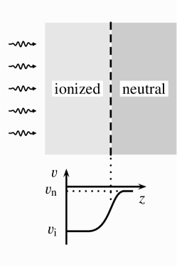
Advection of material through the ionization front may be expected to have various effects on the emission properties of a nebula. In order to simplify the discussion, we will consider a plane-parallel nebula, illuminated at one face by a given radiation field and in a frame of reference in which the ionization front is at rest. This is illustrated in Figure 1a. The gas is supposed to enter the front from the neutral side with velocity and to leave on the ionized side with velocity . Results from this simplified model are described in § 2.2 but we first discuss the relation between this model and real regions.
2.1. Physical Context of Advective Fronts
In this section, we consider two typical scenarios in which advective ionization fronts may be encountered and investigate to what extent they may approximated as steady flows in the frame of reference of the ionization front. In this discussion we follow Shu (1992) in denoting gas velocities in the frame of reference of the ionizing star by , gas velocities in the frame of reference of the ionization front by , and pattern speeds of ionization and shock fronts by .
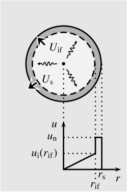
2.1.1 Classical Strömgren Sphere
The evolution of a classical Strömgren-type region in a constant density medium has been described by many authors (e.g., Goldsworthy, 1958; Spitzer, 1978; Shu, 1992; Dyson & Williams, 1997). If the ionizing source turns on instantaneously, then the ionization front is initially R-type and propagates supersonically through the surrounding gas with little accompanying gas motion. By the time the ionization front reaches the initial Strömgren radius (where the rate of recombinations in the ionized region approximately balances the ionizing luminosity of the source), the front propagation velocity has slowed to the order of the sound speed in the ionized gas and the front becomes D-type, preceded by a shock that accelerates and compresses the neutral gas. The initial R-type phase is very short (of order the recombination timescale), and consequently is of little observational importance. The structure of the region during its subsequent D-type evolution is shown in Figure 1b.
(a)
(b)
(c)
The propagation speed of the shock is roughly equal to that of the ionization front and also to the velocity of the gas in the neutral shell:
| (1) |
whereas the ionized gas expands homologously with a velocity that increases linearly with radius, reaching half the speed of the ionization front at the front itself:
| (2) |
Hence, the velocity of the ionized gas immediately downstream of the ionization front in the ionization front frame is
| (3) |
The ionization front propagates very slightly faster than the gas in the neutral shell, giving a small upstream neutral gas velocity in the ionization front frame of
| (4) |
where , are the isothermal sound speeds in the neutral and ionized gas, respectively. The evolution of the ionization front propagation speed can be described in terms of its radius as
| (5) |
where is the initial Strömgren radius. The Mach number reached by the ionized gas just inside the ionization front, measured in the frame of reference in which the front is stationary, is given by . This is plotted in Figure 2 as a function of ionization front radius. During the lifetime of a typical O star (and assuming an ambient density of order ), the radius of a classical region will expand by roughly a factor of 4, so, as can be seen from Figure 2, –0.5 is typical of the majority of the evolutionary lifetime.

2.1.2 Photoevaporation Flow
Photoevaporation flows are very common in ionized regions, occurring whenever the ionization front is convex from the point of view of the ionizing source, thus allowing the ionized gas to freely stream away from the front. Examples include bright-rimmed globules and proplyds in regions and cometary knots in planetary nebulae. On a larger scale, blister-type regions can also be considered photoevaporation flows (Bertoldi & Draine, 1996).
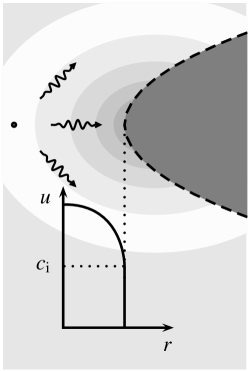
Figure 1c show the structure of an idealized photoevaporation flow, roughly corresponding to the equilibrium cometary globules of Bertoldi & McKee (1990). The neutral gas is assumed to be approximately at rest with respect to the ionizing source and the ionization front to be D-critical with . The ionization front eats slowly into the neutral gas with , and the Mach number reached by the ionized gas at the front will be . Outside the front, the ionized gas accelerates as an approximately isothermal wind, as observed around the Orion proplyds (Henney & Arthur, 1998).
2.2. Direct and Indirect Effects of Advection
In order to provide some physical insight into advective ionization fronts and to guide the interpretation of the numerical simulations, we have developed a simple analytic model for a plane-parallel weak-D ionization front, in which the gas temperature is assumed to be a prescribed monotonic function of the hydrogen ionization fraction, . With this assumption, and considering mass and momentum conservation, it is possible to find algebraic solutions for the density, gas velocity, and sound speed as functions of (see Appendix A). These solutions form a one-parameter family characterized by the maximum Mach number of the gas in the rest-frame of the ionization front, reached asymptotically as . If we now take into consideration the ionization balance and radiative transfer, one can find a solution for , the ionization fraction as a function of physical depth, by solving a pair of ordinary differential equations.
Apart from the maximum Mach number, , the solutions are found to depend on two dimensionless parameters, and . The first of these, (defined in equation A18), is roughly the ratio of recombination length to mean-free-path of ionizing photons in a D-critical front and is not expected to vary greatly between regions, having a typical value of . The second parameter, (defined in equation A17), is roughly the ratio of the thickness of the fully ionized slab to the thickness of the ionization front and is proportional to the ionization parameter at the ionized face: , where . The global importance of advection for the system as a whole can be characterized by the parameter , defined as the ratio of the flux of hydrogen atoms through the ionization front to the flux of ionizing photons at the illuminated face of the slab (equations A10 and A19). For small values of , its value can be approximated as . This can be understood as follows: the local effects of advection at the ionization front itself are always substantial (so long as is not too small), being of order . On the other hand, the partially-ionized zone occupies only a small volume compared with the fully ionized gas unless the ionization parameter is small, so the global effects of advection are reduced by a factor of .
(a)

(b)

Detailed results are calculated in Appendix A for both a low ionization parameter model () and a high ionization parameter model (). The structure of these models for different values of is shown in Figure 3. In the low- model, the direct global effects of advection are expected to be significant and indeed the thickness of the ionized slab is reduced by 50% as approaches unity. In the high- model (more representative of typical regions), the direct global effects of advection are expected to be negligible since . However, we find that even in this case the thickness of the ionized slab varies by about 5% as is varied between 0 and 1. This is due to a pronounced peak that develops in the electron density distribution at the ionization front for (for a static model the electron density declines monotonically through the front). We also find that the ionization front becomes substantially sharper as is increased, which is due to a decrease in the ionization fraction for a given value of the optical depth to ionizing radiation. Both these indirect effects of advection have significant effects on the emissivity profiles of optical emission lines (see Figure 19 of Appendix A), especially those such as [] and [] that form close to the ionization front. One can also calculate the spectral profiles of emission lines from the models, as shown in Figures 20 and 21 of the Appendix. Again, it is lines that form in the partially ionized zone that show the most interesting behavior. These may show RMS line widths roughly equal to the sound speed and significant velocity offsets, both due to the gas acceleration in the ionization front. The derived widths are roughly four times the thermal width of lines emitted by light metals.
Although this analytic model has provided insight into some of the effects of advection, it is obviously deficient in many respects. Many physical processes have been ignored and in particular the use of a fixed temperature profile does not allow for the fact that itself may be affected by the advected flow.
3. Adding Dynamics to Cloudy
In order to study the structure of advective ionization fronts in greater detail, we need to include a wide range of additional physics. This could be done in a variety of ways, for example by integrating through the steady state equations or by including source terms in a time-dependent hydrodynamic simulation. In each case, an implicit treatment of the source terms is necessary, as the many physical processes with timescales shorter than the dynamical timescale lead to the problem being very stiff.
In the present work, we have chosen to adapt the photoionization code, Cloudy, which already includes a comprehensive treatment of the physical source terms. Cloudy, in common with other traditional plasma codes, searches for equilibrium solutions of the ionization equations. In order to treat steady advective flows, we have included advective source and sink terms in the equilibrium balance equations. The effect of this is that the equilibrium search phase now in fact determines the implicit solution of the advective equations, and so treats short-timescale processes in a stable manner.
In this section, we present the basic equations and outline the methods which we use to solve them.
3.1. Equations
Cloudy takes into account the conservation equations for each species and also the heating and cooling balance under the simplifying assumptions of constant density or constant pressure. This procedure can be summarized as balancing source and sink terms for the ionization and energy equations. For the ionization equation in the static case this can be expressed as
| (6) |
where is the rate of change of the volume density of a particular ionization state, which in equilibrium is equal to zero. The are the rates for ionization (where is a higher state than ) and recombination (where is a lower state than ). and cater for processes not included within the ionization ladder, and are respectively the source of ions from such processes and the sink rate into them. A detailed discussion of the solution method for the ionization networks in the equilibrium case is given in Appendix B.
The general Cloudy solution method works by a series of nested iterations. The innermost loop is the ionization network, external to this is the electron density iteration, which enforces charge neutrality, then the temperature loop, which enforces thermal balance. Finally, an optional outermost iteration loop varies the density to achieve pressure (or more generally momentum flux) balance. The whole system is iterated until convergence within a given tolerance.
Once dynamics is included, the continuity and momentum equations must be added to the set of equations to be solved, kinetic and internal energy transport and pressure work must be taken into account, and advection terms must be added to the ionization balance equations. For example, for a plane-parallel steady-state flow (the simplest case, but one that is applicable to blister regions), the equations to solve in flux conservative form are
| (7) |
| (8) |
| (9) |
| (10) |
Here, is an acceleration e.g., gravity or radiation driving, is the specific enthalpy , where is the specific internal energy, and is heating minus cooling. Here the specific internal energy includes only the thermal energy of translation, so , as transfers from other physical energy components (ionization energy, binding energy, vibration and rotation energy of molecules, etc.) are treated as explicit heating and cooling terms in the underlying thermal balance scheme.
The advection terms have the general form of (for steady state), where is the advection velocity. This can be written as
| (11) |
3.2. Differencing Scheme
Although it is possible to solve the ionization equations in an explicitly time-dependent way, this is not the best way to proceed. The photoionization terms in the steady-state solution will often have very short timescales, so stability constraints would limit the time step to this short photoionization timescale, and hence cause an extremely slow convergence of the iterative scheme. Instead, we take advantage of the current algorithm used by Cloudy and difference the equations implicitly. Such an implicit scheme has the advantage that the timestep is not limited to the shortest ionization or recombination time, which is clearly unsatisfactory for an astrophysical system in which the dynamical timescales are general much longer than the ionization or recombination timescales.
At iteration , the advection terms may be approximated based on the value in the present zone and an upstream value in the previous full iteration as
| (12) |
where is the value of at position at the th iteration of the scheme, and is an adjustable advection length. For the first iteration no upstream values are available so no advection terms are included in the equations. It is useful to define the look-back operator
| (13) |
for values, such as , given per unit material. Values specified per unit volume need to be scaled to a conserved variable before the look back is applied, so that
| (14) |
This may be thought of as a first-order Lagrange-remap solution for the advection equation.
For the scheme discussed in Appendix B for the ionization ladder, the advective terms may then be included simply as an additional source term,
| (15) |
and sink rate
| (16) |
in the linearized form of the equations, and iterated to find the non-linear solution as in the time-steady case.
The energy balance equation may be treated in a similar manner. Using the mass conservation equation (eq. 7), we have from equation (9)
| (17) |
which may be differenced as
| (18) |
The terms on the left side of this equation may then be treated as additional heating and cooling terms in the temperature solver.
The continuity and momentum equations are more easily dealt with. The continuity equation is taken into consideration simply by eliminating the velocity in terms of in all equations using the substitution
| (19) |
which comes from integrating the general form of equation 7 where indicates plane parallel, cylindrical or spherical geometry, respectively. The initial condition is given at the illuminated face.
The dynamical pressure, which appears in the momentum equation, is taken into account by adding the ram pressure term to the total pressure.
Varying the Advection Length
The advection length, , in this scheme determines the manner in which different processes are treated. The differencing we have chosen has the effect that processes far more rapid than are treated as in static equilibrium, while slower processes are followed exactly. The correct steady-state solution is found in the limit , but the smaller the advection length chosen, the longer the system will take to reach an equilibrium state. The natural procedure is then to use a first iteration solution by ignoring the advection terms, and then gradually decrease until , where is the size of a spatial zone in the simulation, at which stage the treatment of advection will be as accurate as that of photoionization.
In order to track the convergence of the models and to determine when to reduce the advective timestep, we monitor the behavior of two error norms, and . Both are calculated as the squared norm over all zones, , and ionic/molecular species, . The first of these norms is the convergence error, defined as
| (20) |
which measures the difference between the model solutions for the last two iterations. The second is the discretization error, defined as
| (21) |
which measures the accuracy of the present estimate of the advective gradients in the solution compared to an estimate with half the advection length.
If , then the solution is converged with the present , while if the errors in the Lagrangian estimate of the gradient of the value are still significant, then the timestep should be decreased. Cutting when produces substantial improvements in the rate of convergence of the advective solutions. However, it can still take a substantial number of iterations to reach equilibrium for large advection velocities.
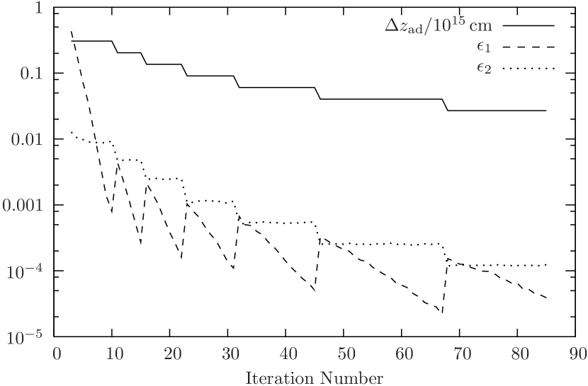
An example of the way in which , , and vary during a model calculation is given in Figure 4 (which corresponds to model ZL009 discussed in the following section). It can be seen that while remains constant, the convergence error, , decreases with each iteration, while hardly changes after the first iteration for a given . When falls to a low enough value, then all physical processes that occur on timescales longer than have converged, so the advection length can be reduced. This has the effect of lowering but also temporarily increases due to the release of shorter-timescale processes from strict local equilibrium, so several iterations must be carried out at the new value of . This procedure is continued until has fallen to a sufficiently low value.
4. Results
In this section we present results for selected advective ionization fronts calculated using Cloudy, all using a plane-parallel slab geometry. The principal input parameters for the models are the hydrogen number density, , gas velocity, , hydrogen-ionizing photon flux, , all specified at the illuminated face. The spectral distribution of the incident radiation field was assumed to be a black body with effective temperature, . All these parameters are shown in Table 1 for the three models presented here. The gas-phase elemental abundances for all the models were set at the standard ISM values (Baldwin et al., 1996) and Orion-type silicate and graphite grains were included (Baldwin et al., 1991). Since this paper is concerned with the effects of advection on the ionization front, all molecules were turned off and the integration was stopped when the electron fraction fell below . The inclusion of molecular processes in the PDR will be described in a following paper. The models also include an approximate treatment of a tangled magnetic field (see Appendix C), characterized by the field strength at the illuminated face, .
One further physical process was disabled in these models: the radiative force due to the absorption of stellar continuum radiation (principally by dust grains). This was done for purely pragmatic reasons, since the inclusion of this process for high ionization parameter models makes it very difficult to set the approximate desired conditions at the ionization front by varying conditions at the illuminated face. Models that do include this process are discussed further in section 5.2.
The first two models, ZL009 and ZH007, are weak-D fronts with low and high ionization parameter, respectively, with parameters similar to the toy models discussed in Appendix A. The velocity at the ionized face, , was set somewhat below the isothermal sound speed in order to avoid the possibility of gas passing through a sonic point during an intermediate iteration (transonic fronts will be considered in a following paper). The third model, ZH050, is a weak-R front in which the gas velocity relative to the front is supersonic throughout. Such R-type fronts are likely to be transient and thus of limited observational significance. Nevertheless, this model is useful since it provides a stringent test of our simulations in the limit of high advective velocities.
As well as the advective models, we also calculate equivalent static models for each of the three cases considered, which have constant pressure for comparison with the weak-D fronts or constant density for comparison with the weak-R front.
| Parameter | ZL009 | ZH007 | ZH050 |
|---|---|---|---|
| none | |||
| 9.9 | 6800 | 6800 | |
| 8.1 | 13.8 | 13.8 | |
| 2.2 | 0.0015 | 0.008 |
4.1. Low Ionization Parameter, Weak-D


This model, ZL009, has physical parameters that are inspired by those of cometary globules in planetary nebulae such as the Helix, although the geometry is plane-parallel rather than spherically divergent. The ionization parameter of the model is very low (), which accentuates the global effects of advection and also leads to the ionization front thickness being comparable to the Strömgren thickness of the ionized layer.
As can be seen from Figure 5, the advection has large effects on the model structure as would be expected given the large value of . The depth of the ionized region is reduced by more than a factor of two with respect to the static model, with concomitant reductions in the brightness of the hydrogen recombination lines (see Table 2). The collisional lines of [], [], and [] are also reduced in intensity, albeit to a lesser degree ([] emission from this model is negligible due to the low ionization parameter). Interestingly, the intrinsic Balmer decrement is increased in the advective model, which gives (reddening by internal dust is not included in the line ratios given in Table 2). This is because the temperature at low ionization fractions is significantly higher in the advective model, which leads to a non-negligible collisional contribution to the Balmer emission that preferentially excites H. The temperature in the more highly ionized zone is also increased somewhat by the effects of advection.
| Model ZL009 | Model ZH007 | |||||||||
| Line Intensity | Line Intensity | |||||||||
| Line | Static | Advect | Static | Advect | ||||||
| [] | ||||||||||
| [] | ||||||||||
| [] | ||||||||||
| [] | ||||||||||
Also listed in Table 2 are the mean velocities and full-width-half-maxima of the different emission lines, calculated assuming that the model is observed face on. The emission line profiles are illustrated in Figure 7. The contribution from each computational zone to the line profile is thermally broadened using the local temperature and the atomic weight of the emitting species. As a result, the line is significantly broader than the collisionaly excited metal lines. The [] line is blue shifted with respect to [] and [], which is due to the acceleration of gas through the ionization front, as can be seen in Figure 5a. The line has two components: a broad blue-shifted component due to emission from the ionized flow, and a narrow component at zero velocity, caused by a subsidiary peak in the electron density that occurs at low ionization fractions where the temperature changes sharply.
For the [] line, the thermal broadening and the gas acceleration both contribute in equal amounts to the predicted line width. For the lighter metal lines, the acceleration broadening remains roughly the same but the thermal width is increased somewhat. For , the thermal broadening dominates.
In this model, the gas velocity and Mach number increase monotonically as the gas flows from the neutral to the ionized side, reaching a maximum Mach number of at the illuminated face. As a result, emission lines from more highly ionized species are more blue-shifted (see Table 2). However, the effect is slight with only velocity difference between [] and [].
4.2. High Ionization Parameter, Weak-D


This model, ZH007, has physical parameters (see Table 1) inspired by the central region of the Orion nebula (Baldwin et al., 1991). The density is only slightly higher than in ZL009 but the ionizing flux is much higher, resulting in a far higher ionization parameter (). The ionization front is much thinner than the depth of the fully ionized slab. The local advection parameter, (see Section 2 and Appendix A), is somewhat higher than in the previous model due to the hotter gas temperature and softer ionizing spectrum but the much higher value of that accompanies the higher ionization parameter means that the global advection parameter, , is very small.
The structure of the advective model as a function of depth into the slab from the illuminated face is shown by solid lines in Figure 8. For some panels, an equivalent constant-pressure, static model is also shown (dashed lines). The indirect effects of advection are much greater than the direct loss of 0.1% of the incident ionizing flux due to the ionization of fresh gas. The largest effect is a roughly 3% increase in the mean density in the ionized zone (the densities at the illuminated faces are set equal in the static and advective models) due to the varying importance of ram pressure as the velocity varies through the slab. Due to the difference in density dependence of recombination and dust absorption, this leads to a slight decrease in the ionized column density together with an increase in the emission measure, caused by a reduction in the fraction of ionizing photons that are absorbed by dust grains.
Figure 9 shows some of the same quantities as in Figure 8 but this time plotted against the electron fraction, . This effectively ‘zooms in’ on the ionization front transition itself, allowing one to appreciate details of the structure that are not apparent in the plots against depth. Note that the more neutral gas is on the left in Figure 9, whereas it was on the right in Figure 8. In Figure 9b, which shows the temperature profiles, it can be seen that the initial heating of the gas as it is ionized is more gradual in the advective model than in the static model due to the photo-heating timescale being longer than the dynamic timescale. However, once the ionization fraction exceeds about 20% the photo-heating rate exceeds the static equilibrium model because the neutral fraction at a given value of the ionizing flux is higher than in the static case. This produces a characteristic overheating, which is often seen in advective fronts. In the current case it is relatively modest, producing an extended plateau for –0.9. For the gas approaches static thermal equilibrium again and the two curves coincide with temperature variations determined by radiation hardening and the varying importance of the diffuse field. Figure 9c shows the variation in the gas density and it can be seen that the density on the far neutral side is significantly higher in the advective model. This is a result of the lack of ram pressure on the neutral side (see Figure 9e), which means the thermal pressure must increase to compensate. The magnetic field at the illuminated face in this model was set to be , implying a negligible contribution to the total pressure in the ionized gas. However, on the far neutral side, where the density is higher the field is much larger (assumed to grow with compression as , see Appendix C), so that the magnetic pressure becomes appreciable, limiting the density in the cold gas. The inferred in the neutral gas is similar to observed values in the neutral veil of Orion (Troland et al., 1989).
The line emissivities as a function of depth for the ZH007 model are shown in Figure 10. The main change between the static and advective models is the sharp peak at the ionization front that is seen in the emissivity of lines from singly-ionized species such as []. This peak is due to the electron density peak seen in Figure 3 and discussed in Appendix A.
The integrated emergent emission line spectrum (Table 2) is barely affected by the advection. As a result of the increase in emission measure discussed above, although the ionization front moves appreciably inward (Figure 8d), the Balmer line flux is actually slightly higher in the advective model than in the static model. On the other hand, lines that form in the ionization front itself, such as [] and [], are somewhat reduced in intensity in the advective model due to the narrowing of the ionization front by advection (see discussion in Appendix A).
Unlike in the the low ionization parameter model of the previous section, in this model the velocity and Mach number do not increase monotonically from the neutral to the ionized side. Instead, the maximum Mach number (), which also corresponds to the maximum velocity, occurs at the He0/He+ front. Although this does not correspond to the maximum temperature, it is a maximum in the sound speed due to the decrease in the mean mass per particle when He is ionized. There is a second, slightly lower, maximum in the sound speed, Mach number, and velocity just inside the H ionization front where radiation hardening causes a temperature maximum. The velocity also starts to increase again very close to the illuminated face.
4.3. High Ionization Parameter, Weak-R
This model, ZH050, is identical to ZH007 except that the gas velocity at the illuminated face is set to , producing a weak-R front. The model structure as a function of depth is shown in Figure 12 and as a function of electron fraction in Figure 13. In both cases, the advective model is now compared with a constant-density static model as opposed to the constant-pressure model that was used for comparison with the weak-D models. As can be seen from Figure 12a and c the velocity and density are roughly constant across the front, as is expected in the weak-R case. The extremal Mach number in the front (which for R-type fonts is a minimum, see Appendix A) is , which occurs on the ionized side of the front (see Fig. 13c) at .
4.4. Temperature Structure of the Ionization Fronts
Figure 12b shows that our weak-R model has a pronounced temperature spike at the ionization front, together with a smaller spike at the He ionization front. Figure 13b shows that this is a more extreme manifestation of the overheating in the ionization front that was seen in the weak-D model (Fig. 9b). However, even in this case of a rapidly propagating front we do not find the overheating to be very great, reaching a maximum temperature of only . Other authors have found more pronounced over-heating effects in dynamic ionization fronts (Rodriguez-Gaspar & Tenorio-Tagle, 1998; Marten & Szczerba, 1997) but for different values of the physical parameters. Marten & Szczerba found temperatures as high as behind R-type fronts moving at a substantial fraction of the speed of light, which would be difficult to model using our steady-state code. Rodriguez-Gaspar & Tenorio-Tagle studied the time-dependent evolution of an region after the turning-on of an O star, finding temperatures of order behind the ionization front soon after its transition from R to D-type. Their higher temperatures may be due to these authors including fewer cooling processes than are included in Cloudy (for further discussion, see Williams & Dyson, 2001, and references therein). The greater width of the temperature spike in the Rodriguez-Gaspar & Tenorio-Tagle models is due to the fact that they were considering lower densities, so the gas moves further from the ionization front in the time it takes to cool to the equilibrium temperature.


5. Discussion
In this section, we look for evidence of advective effects in one of the closest and best-studied regions, the Orion nebula. We concentrate on the clearest signatures of advection to emerge from our simulations: the electron density spike and the ionization-resolved kinematics.
5.1. Electron Density Structure of the Orion Bar
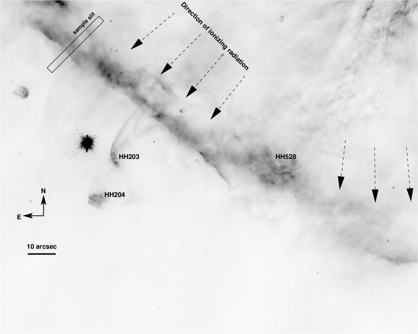

One firm prediction of the advective model that differs from the static case is the existence of a sharp electron density peak at the position of the ionization front. This peak manifests itself most clearly in the emission of the [] line (see Figure 10), producing a narrow emissivity peak at the edge of the broader peak that comes from the neutral Helium zone. In Figure 14 we show an [] image of the bright bar region in the Orion nebula that shows evidence of just such a structure.111This image is based on data obtained with the WFPC2 instrument on the Hubble Space Telescope, provided by C. R. O’Dell. The bar is believed to be a section of the principal ionization front in Orion that is seen almost edge-on. It can be seen as a diffuse strip of [] emission () stretching from the top-left to bottom right of the image. The principal source of ionizing radiation is the O7V star Ori C, located off the image to the NW. A sharp, bright edge to the emission can be seen on its SE side along a considerable fraction of the bar, which may correspond to the electron density peak.
The geometry of the nebula in the vicinity of the bar is far more complicated than the plane-parallel geometry assumed in the models, making a quantitative comparison difficult. The bar probably consists of at least two overlapping folds in the ionization front and its appearance is also affected by protruding fingers of neutral gas and interactions with the HH 203/204 and HH 528 jets. However, the straight region of the bar to the NE of the HH 203/204 bowshocks show a relatively simple structure, which we will attempt to compare with our model predictions. We present in Figure 15 emission line spatial intensity profiles along a short section of narrow slit parallel to the bar, with position as indicated in Figure 14. Comparison of Figure 15 with the model profiles of Figure 10 shows good general agreement.
The electron density in the bar region has been measured from the [] line ratio to be around (Wen & O’Dell, 1995; García Díaz & Henney, 2003), whereas model ZH007 predicts a value of for the []-derived density. On the other hand, the incident ionizing flux can be estimated to be about , which is half that of the model ZH007. Thus the model has the same ionization parameter as the bar and the results can be directly compared by multiplying the model lengths by a factor of two such that the spatially broad component to the [] emission is predicted to have a thickness of , in reasonable agreement with what is observed. The electron density peak at the ionization front is predicted to have a thickness of , which is also very close to the observed thickness of the narrow ridge in [] (note that this thickness is fully resolved by the HST, which has an angular resolution of at optical wavelengths).
5.2. Velocity-Ionization Correlation in the Orion Nebula
The mean velocity of different optical emission lines from the core of the Orion nebula has long been known to correlate with the ionization potential of the parent ion (Kaler, 1967; O’Dell et al., 1993; Henney & O’Dell, 1999; O’Dell et al., 2001; Doi et al., 2004). Lines from more highly ionized species such as are blue-shifted by approximately with respect to the molecular gas of OMC-1, which lies behind the nebula, with intermediate-ionization species such as [] being found at intermediate velocities.
The results of section 4 show that just such a correlation can be qualitatively reproduced by our models. However, on closer inspection, many significant differences are revealed between the model results and the Orion observations. A much clearer velocity-ionization correlation exists in model ZL009 (low ionization parameter) then in ZH007 (high ionization parameter, more pertinent to the Orion nebula), as can be seen from Table 2 and Figures 7 and 11. This is not surprising since the emission in the high ionization parameter model is dominated by ionized equilibrium gas, where velocity changes are rather small and are driven by variations in the thermal balance (the complex interplay of radiation hardening and the excitation of different coolant lines) rather than being directly caused by ionization changes. Furthermore, both the magnitude of the velocity shifts seen in the models and the broadening induced by the gas acceleration are somewhat smaller than is observed in Orion.
In order to better reproduce the observations, what is required is a means of continuing the acceleration of the gas inside the body of the nebula, where hydrogen is fully ionized. There are two means by which this might be achieved: first, by including the continuum radiation force upon the ionized gas/dust mixture, or, second, by considering a transonic strong-D ionization front in a non-plane, divergent geometry.

The results of a model that includes the continuum radiation force are shown in Figure 16. The thick line in the lower panel shows the integral along the radiation propagation direction of the radiative force per unit volume, , that acts on the material in the flow.222The dust-gas drift velocity is always much slower than the flow velocity in these models, so it is valid to suppose that the gas and dust dynamics are perfectly coupled. In response to this radiative forcing, the total pressure increases with depth and, since the flow is subsonic, the gas pressure and density increase in the same direction. By mass conservation, this leads to an acceleration of the gas towards the illuminated face, as can be seen in Figure 16a (compare Figure 8a, where this process is absent).
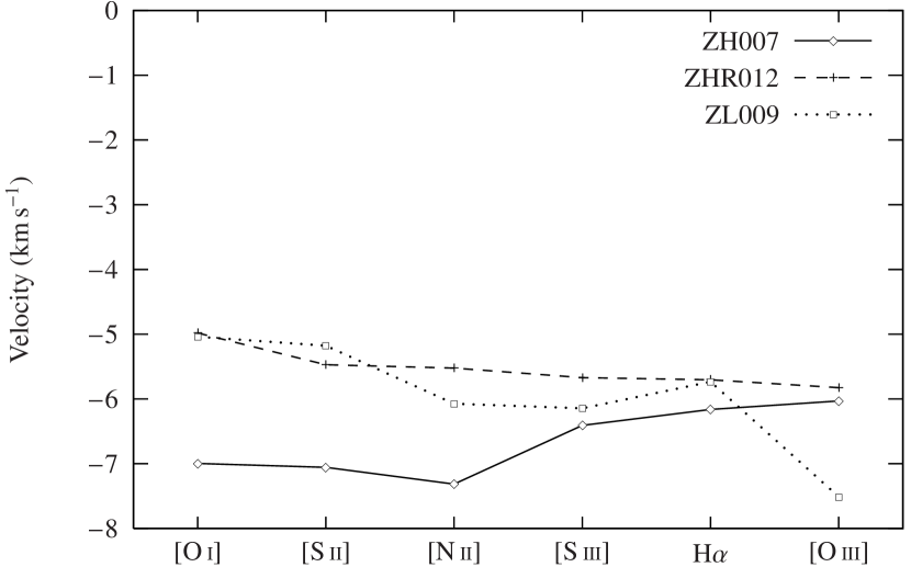
However, this acceleration of the fully-ionized gas does not have a very large effect on the mean velocity of the emission lines, as can be seen from Figure 17. This is because the higher-velocity gas represents only a small fraction of the total emission, even for the [] line. Although the model ZHR012 does show a clear relation between velocity and ionization (unlike ZH007), the gradient is very small, being less than between [] and [], compared with an observed difference of 5 to in the Orion nebula. Also, any deviations from a strictly face-on orientation of the observer would tend to reduce the observed gradients.
In order to reproduce the observed kinematics of the Orion nebula, one needs a strong acceleration of the gas in the region between the hydrogen and helium ionization fronts, since this is the region where the ionization of heavy elements such as oxygen and sulfur is changing most swiftly. We have shown that it is not possible to achieve this with a plane-parallel model. In such a geometry, gas acceleration requires either a gradient in the sound speed or the application of a body force, neither of which are present with the required magnitude in the relevant region. Strong changes in the sound speed only occur at greater depths, in the hydrogen ionization front, while the effective gravity associated with continuum radiation pressure acts mainly at shallower depths, where the heavy-element ionization is not changing.
On the other hand, as we will show in a following paper, the requisite acceleration is a natural consequence of models in which the flow is divergent (either spherical or cylindrical) rather than plane-parallel. Although such models are obviously relevant to such objects as proplyds (Henney & O’Dell, 1999) and photoevaporating globules (Bertoldi & McKee, 1990), it is not so apparent that they should apply to the large-scale emission from the Orion nebula, which has been traditionally visualized as a bowl-like cavity on the near side of the molecular cloud OMC-1. However, three-dimensional reconstruction of the shape of the ionization front (Wen & O’Dell, 1995) indicates that the radius of curvature of the front is larger than its distance from the ionizing star. In such a case, the divergence of the radiation field can lead to a (weaker) divergence of the flow (Henney, 2003). Another possibility is that the mean flow is the superposition of multiple divergent flows from the many bar-like features that have been found in the nebula (O’Dell & Yusef-Zadeh, 2000).
6. Conclusions
In this paper, we have developed a method for including the effects of steady material flows in the plasma physics code Cloudy (Ferland, 2000), which was previously capable of modeling only static configurations. We have presented a detailed description of the numerical algorithms and an example application to the restricted problem of plane-parallel ionization-bounded regions where the flow does not pass through a sonic point (weak fronts). The most important conclusions from our study are as follows:
-
1.
The local effects of advection are most important in those regions of the flow where physical conditions are strongly varying over short distances, such as in the hydrogen ionization front.
-
2.
The global effects of advection on an region depend on the relative thicknesses of the ionization front and the region as a whole, which is a function of the ionization parameter. Only for low values of the ionization parameter, such as are found in cometary knots of planetary nebulae, do we find a significant direct effect of advection on the emission properties integrated over the entire the region. For higher ionization parameters, more typical of regions around O stars, the effects of advection are indirect and more localized.
-
3.
One such indirect effect is a modification of the temperature structure in the ionization front due to the overheating of partially ionized gas. However, we find the magnitude of this effect to be much less than has previously been claimed (Osterbrock, 1989; Rodriguez-Gaspar & Tenorio-Tagle, 1998), probably due to our more realistic treatment of heating and cooling processes. For weak D-type fronts (subsonic flows), the temperature reached in the front does not exceed the equilibrium temperature in the fully ionized gas (see Figure 9b). Even for supersonic R-type fronts, the peak temperature is only about 20% higher than the equilibrium ionized value (see Figure 13b). The temperature increase causes an increase in the peak emissivity of the [] line, but the total emission of this line tends to be less than in an equivalent static model because advection acts to sharpen the ionization front and hence decreases the width of the zone where [] is emitted.
-
4.
Another indirect effect of advection in high ionization parameter regions is the production of a sharp spike in the electron density, which occurs at the ionization front whenever the peak Mach number in the flow exceeds about 0.5. This spike does not occur in static models and its existence can be shown analytically to be a consequence of the exchange between thermal pressure and ram pressure as the gas is accelerated through the front (Appendix A, Figure 18). As such, it can serve as a useful diagnostic for the presence of advection in ionization fronts, best observed in the [] line, for which advective models predict a two-component structure (Figure 10b): a broad peak of emission from the equilibrium H+-He0 zone plus a narrower peak from the spike at the ionization front. Just such a structure is seen in HST images of the Orion bar (Section 5.1), suggesting that advection is important in that region.
-
5.
Finally, the advective models provide a mapping between the ionization state of the gas and its velocity and can hence be used to predict kinematic profiles of different emission lines, which can be compared with spectroscopic observations. We make such a comparison in the case of the Orion nebula but find that the plane-parallel models presented in this paper are utterly incapable of explaining the observed kinematics (Section 5.2). The observations seem to demand a strong acceleration of the gas in the region between the hydrogen and helium ionization fronts, whereas the only acceleration mechanisms that can act in the plane-parallel models either occur at greater depths (gas heating in the hydrogen ionization front) or at shallower depths (effective gravity due to continuum radiation pressure).
The work presented in this paper forms a basis for further development of dynamic photoionization models that will be covered in two following papers. In the first, the inclusion of chemistry and dissociation/formation processes allows a unified treatment of the entire flow from cold, molecular gas, through the PDR, and into the region. Previous work by Stoerzer & Hollenbach (1998) indicates that advection can have a significant effect on the position of the molecular hydrogen dissociation front. In the second, divergent, transonic flows from strong-D fronts are modeled, which can explain the kinematic observations discussed in paragraph 5 above.
References
- Baldwin et al. (1996) Baldwin, J. A., Crotts, A., Dufour, R. J., Ferland, G. J., Heathcote, S., Hester, J. J., Korista, K. T., Martin, P. G., O’Dell, C. R., Rubin, R. H., Tielens, A. G. G. M., Verner, D. A., Verner, E. M., Walter, D. K., & Wen, Z. 1996, ApJ, 468, L115+ [ADS]
- Baldwin et al. (1991) Baldwin, J. A., Ferland, G. J., Martin, P. G., Corbin, M. R., Cota, S. A., Peterson, B. M., & Slettebak, A. 1991, ApJ, 374, 580 [ADS]
- Bertoldi & Draine (1996) Bertoldi, F. & Draine, B. T. 1996, ApJ, 458, 222
- Bertoldi & McKee (1990) Bertoldi, F. & McKee, C. F. 1990, ApJ, 354, 529
- Doi et al. (2004) Doi, T., O’Dell, C. R., & Hartigan, P. 2004, AJ, 0, 0
- Dyson & Williams (1997) Dyson, J. E. & Williams, D. A. 1997, The physics of the interstellar medium, The graduate series in astronomy (Bristol: Institute of Physics Publishing)
- Ferland (2000) Ferland, G. J. 2000, in Astrophysical Plasmas: Codes, Models, and Observations, (Eds. S. J. Arthur, N. Brickhouse, and J. Franco) Revista Mexicana de Astronomía y Astrofísica (Serie de Conferencias), Vol. 9, 153–157 [ADS]
- Ferland et al. (1998) Ferland, G. J., Korista, K. T., Verner, D. A., Ferguson, J. W., Kingdon, J. B., & Verner, E. M. 1998, PASP, 110, 761 [ADS]
- García Díaz & Henney (2003) García Díaz, M. T. & Henney, W. J. 2003, in Winds, Bubbles and Explosions, (Eds. S. J. Arthur and W. J. Henney) Revista Mexicana de Astronomía y Astrofísica (Serie de Conferencias), Vol. 15, 201–201
- Goldsworthy (1958) Goldsworthy, F. A. 1958, Reviews of Modern Physics, 36, 1062
- Goldsworthy (1961) —. 1961, Phil. Trans. A, 253, 277
- Harrington (1977) Harrington, J. P. 1977, MNRAS, 179, 63
- Henney (2003) Henney, W. J. 2003, in Winds, Bubbles and Explosions, (Eds. S. J. Arthur and W. J. Henney) Revista Mexicana de Astronomía y Astrofísica (Serie de Conferencias), Vol. 15, 175–180
- Henney & Arthur (1998) Henney, W. J. & Arthur, S. J. 1998, AJ, 116, 322 [ADS]
- Henney & O’Dell (1999) Henney, W. J. & O’Dell, C. R. 1999, AJ, 118, 2350 [ADS]
- Kahn (1954) Kahn, F. D. 1954, Bull. Astron. Inst. Netherlands, 12, 187
- Kaler (1967) Kaler, J. B. 1967, ApJ, 148, 925
- López-Martín et al. (2001) López-Martín, L., Raga, A. C., Mellema, G., Henney, W. J., & Cantó, J. 2001, ApJ, 548, 288 [ADS]
- London (1978) London, R. 1978, ApJ, 225, 405
- Marten & Szczerba (1997) Marten, H. & Szczerba, R. 1997, A&A, 325, 1132 [ADS]
- Natta & Hollenbach (1998) Natta, A. & Hollenbach, D. 1998, A&A, 337, 517 [ADS]
- Newman & Axford (1968) Newman, R. C. & Axford, W. I. 1968, ApJ, 151, 1145
- O’Dell (2001) O’Dell, C. R. 2001, ARA&A, 39, 99 [ADS]
- O’Dell et al. (2001) O’Dell, C. R., Ferland, G. J., & Henney, W. J. 2001, ApJ, 556, 203 [ADS]
- O’Dell et al. (1993) O’Dell, C. R., Valk, J. H., Wen, Z., & Meyer, D. M. 1993, ApJ, 403, 678
- O’Dell & Yusef-Zadeh (2000) O’Dell, C. R. & Yusef-Zadeh, F. 2000, AJ, 120, 382
- Osterbrock (1989) Osterbrock, D. E. 1989, Astrophysics of gaseous nebulae and active galactic nuclei (Mill Valley, CA: University Science Books)
- Press et al. (1992) Press, W. H., Teukolsky, S. A., Vetterling, W. T., & Flannery, B. P. 1992, Numerical recipes in FORTRAN. The art of scientific computing (Cambridge University Press)
- Redman et al. (1998) Redman, M. P., Williams, R. J. R., Dyson, J. E., Hartquist, T. W., & Fernandez, B. R. 1998, A&A, 331, 1099 [ADS]
- Richling & Yorke (2000) Richling, S. & Yorke, H. W. 2000, ApJ, 539, 258 [ADS]
- Rodriguez-Gaspar & Tenorio-Tagle (1998) Rodriguez-Gaspar, J. A. & Tenorio-Tagle, G. 1998, A&A, 331, 347 [ADS]
- Sankrit & Hester (2000) Sankrit, R. & Hester, J. J. 2000, ApJ, 535, 847 [ADS]
- Scowen et al. (1998) Scowen, P. A., Hester, J. J., Sankrit, R., Gallagher, J. S., Ballester, G. E., Burrows, C. J., Clarke, J. T., Crisp, D., Evans, R. W., Griffiths, R. E., Hoessel, J. G., Holtzman, J. A., Krist, J., Mould, J. R., Stapelfeldt, K. R., Trauger, J. T., Watson, A. M., & Westphal, J. A. 1998, AJ, 116, 163 [ADS]
- Shapiro & Raga (2001) Shapiro, P. R. & Raga, A. C. 2001, in Revista Mexicana de Astronomia y Astrofisica Conference Series, Vol. 10, 109–114
- Shu (1992) Shu, F. H. 1992, Physics of Astrophysics, Vol. II (University Science Books)
- Spitzer (1978) Spitzer, L. 1978, Physical processes in the interstellar medium (New York: Wiley-Interscience)
- Stoerzer & Hollenbach (1998) Stoerzer, H. & Hollenbach, D. 1998, ApJ, 495, 853 [ADS]
- Troland et al. (1989) Troland, T. H., Heiles, C., & Goss, W. M. 1989, ApJ, 337, 342
- Wen & O’Dell (1995) Wen, Z. & O’Dell, C. R. 1995, ApJ, 438, 784
- Williams & Dyson (1996) Williams, R. J. R. & Dyson, J. E. 1996, MNRAS, 279, 987 [ADS]
- Williams & Dyson (2001) —. 2001, MNRAS, 325, 293 [ADS]
- Williams et al. (2000) Williams, R. J. R., Dyson, J. E., & Hartquist, T. W. 2000, MNRAS, 314, 315 [ADS]
Appendix A Simplified Analytic Model for Weak-D Ionization Fronts
In this appendix, we develop a simple analytic model for a plane-parallel ionization front in order to explore the most important effects of advection upon the front structure. The principal simplification involved is the assumption that the gas temperature, , follows a unique prescribed function of the hydrogen ionization fraction, . It is a generic property of ionization fronts that the temperature tends to increase as one passes from the neutral to the ionized side of the front. In the analytic model, we assume that the increase is monotonic and has the form:
| (A1) |
where is the limiting temperature in the ionized gas (), is the limiting temperature on the far neutral side (), and is a parameter controlling the sharpness of the transition. In reality, for moderate to high ionization parameters, the hardening of the radiation field as one approaches the ionization front causes the temperature to have a maximum for somewhat less than unity (see, for example, Figure 9b). However, for weak-D fronts, equation (A1) is sufficient to capture the main effects of advection.333For D-critical/strong-D fronts, on the other hand, the position of the temperature maximum is critical.Also, it turns out that advection itself will modify the curve (see Section 4) but, again, we ignore this complication in the analytic model. We further simplify the model by only considering the ionization of hydrogen and ignoring the effects of radiation pressure, dust, and magnetic fields.
With these approximations, the gas pressure is given by
| (A2) |
where is the hydrogen number density. For a static front, the gas pressure will be constant, so it is a simple matter to calculate the variation of gas density, , and electron density, , with ionization fraction:
| (A3) |
These are all plotted as solid lines in Figure 18. In this and all following examples, we use temperature-law parameters of and , which agrees within 10–20% with the temperature profiles of all the weak-D models in section 4. It can be seen that, although the gas density declines with increasing , the electron density is a monotonically increasing function of (this is always true, whatever the value of ).

In order to calculate the structure of a non-static, dynamic front it is necessary to consider the conservation of mass and momentum, which are given, in plane-parallel geometry, by
| (A4) |
where is the gas velocity and and are the (constant) mass and momentum fluxes. It is convenient to define the dimensionless variable :
| (A5) |
which, by equations (A4), is related to the isothermal Mach number () via
| (A6) |
with the inverse relation
| (A7) |
in which the sign applies to a subsonic flow and the sign to supersonic flow.
Equation (A6) shows that everywhere and that corresponds to the sonic point: . A given ionization front can be characterized by the parameter , which is the minimum value of anywhere in the front. This is achieved when the isothermal sound speed attains its maximum value , and, in the case of the weak-D fronts considered here, corresponds to the maximum value of the (subsonic) Mach number: .444For R-type fronts, on the other hand, is the minimum Mach number. For D-critical and strong-D fronts, and is no longer a turning point in , not even a point of inflexion, although is still a maximum in . For a temperature profile such as equation (A1), occurs at and the sound speed varies with as
| (A8) |
It can be seen that all weak-D fronts with a given form a one-parameter family, characterized by their maximum Mach number . For a given , the corresponding can be calculated from (A6) and then from (A5) we have , which can be inserted into (A7) to give , from whence we also have , , and . Hence, the full structure of the ionization front as a function of can be found algebraically. The results are plotted in Figure 18 for various weak-D fronts between and .
For , the velocities are everywhere very subsonic and the density structure is hardly any different from the static case (lower panels). In this regime, the velocity rises approximately as . There is hence an initial brisk acceleration for , driven largely by the increase in , followed by a slower, almost constant, acceleration, driven largely by the increase in ion fraction. For higher , the gas density contrast between the ionized and neutral sides increases and for this causes there to be a maximum in at an intermediate value of . Solutions with also show a second episode of steep acceleration as .
In order to apply these results, it is necessary to find the mapping between the ionization fraction, , and physical position within the ionization front. For this, it is necessary to introduce more parameters than have so far been considered. The ionized gas is assumed to have an inner boundary , at which the ionizing flux is , and with being the distance into the ionized gas, measured from the illuminated face, in the direction of decreasing . Globally, the flux of ionizing photons at must be balanced by the recombinations per unit area, integrated throughout the structure, plus the (constant) flux of hydrogen nuclei through the front:
| (A9) |
where is the recombination coefficient, which we approximate as a power-law in the gas temperature: . The global importance of advection on the ionization balance can be characterized by the relative magnitude of the two terms on the RHS of this equation, so we define a dimensionless “global advection parameter”:
| (A10) |
We also define a characteristic “Strömgren distance” as
| (A11) |
in terms of which, (A9) becomes
| (A12) |
At each point, , within the structure we also have the local ionization equation:
| (A13) |
where is the local value of the ionizing flux and is the mean photo-absorption cross-section for ionizing photons, evaluated by integrating over the ionizing spectrum at that point. The attenuation of the ionizing radiation is expressed by
| (A14) |
Equations (A13) and (A14) can be reexpressed in dimensionless form as
| (A15) |
and
| (A16) |
with dimensionless variables:
Equations (A15) and (A16) also make use of two dimensionless parameters:
| (A17) |
and
| (A18) |
in terms of which the global advection parameter, , can be expressed as
| (A19) |
and whose significance is explored more fully in section 2. These two differential equations can be integrated numerically to find the full solution for the ionization front structure in physical space. Note that for the static case (), (A15) is undefined and we instead have simply that the term in square brackets is zero.
We now present sample results from solving equations (A15) and (A16) using parameters appropriate to an region illuminated by an O star. We approximate the reduction in photoabsorption cross-section due to the hardening of the ionizing radiation field as . This is a good fit to the exact result from assuming the ionizing spectrum of a blackbody and , from which we also obtain . We also assume , , which give . For the parameter , we adopt the values and , corresponding to a low and a high ionization parameter, respectively, with the second being more representative of typical regions. The results are shown in Figure 3. In each case, curves of the electron density and gas velocity are shown for models with (right to left) , , , , , . For the direct effects of advection are considerable, since , so that for the higher Mach numbers a substantial fraction of the incident ionizing flux is consumed by ionization of new atoms, which pushes the ionization front to the left.
It can also be seen that the advection decreases the width of the ionization front. In the static front, the width is determined by the mean free path of ionizing photons in the partially ionized gas, which gives , whereas in the advective fronts the ionization fraction at a given value of the ionizing flux is smaller, leading to a sharper front (4 times narrower in the near-critical case). Also, the electron density in the advective models has a peak at the ionization front, which is not seen in the static models. For , we have , so the direct effects of advection on the global properties of the model should be very small. Nonetheless, the ionization front position varies by about 5% between the static model and the model, which is due to the effect of the electron density peak.
In order to investigate the effects of advection on the emission-line properties of the nebula, we consider a generic recombination line with emissivity
| (A20) |
where is the number density of the recombining ion, and a generic collisionally excited line with emissivity
| (A21) |
where is the excitation energy of the upper level and is the collisional de-excitation coefficient. The ion density can be assumed to be for singly-ionized ions and for neutral atoms.

The results are shown in Figure 19, which compares the line emissivities as a function of radius for the model at two values of : 0.0 and 0.99. The total emission from all the lines is significantly reduced in the nearly D-critical model with respect to the static model due to the smaller depth of the ionized zone. On the other hand, the relative intensities integrated over the entire structure change by less than 10%. The peak of the neutral collisional line is much sharpened in the advective model due to the narrowing of the ionization front. In addition, the singly-ionized collisional line and the recombination line both show peaks in their emissivity at the ionization front, which are due to the electron density peak there (see Figure 3).
The line emissivity can be combined with the velocity structure of the front to create synthetic emission line profiles. We assume that the front is observed face-on from the ionized side, so that the lines are all blue-shifted with respect to the neutral gas, which is assumed to be stationary. We calculate the emergent intensity profile, , of an emission line ignoring any optical depths effects:
| (A22) |
where is the observed velocity and is the thermal Doppler width, calculated at each point in the structure assuming typical atomic weights of 16 for the collisional neutral line, 14 for the collisional ionized line, and 1 for the recombination line.
(a)

(b)

The resultant profiles are shown in Figure 20 for the collisional lines.555The recombination line has a very similar emissivity profile to the singly ionized collisional line and the low atomic weight only serves to smear out the details of the line profile. The increasing blue-shift of both lines with increasing maximum Mach number is evident. For the singly-ionized line, there is hardly any dependence of linewidth on the advection strength because most of the emission comes from the almost fully ionized gas, which shows only small velocity gradients. For the neutral line, on the other hand, the nearly critical model shows a much broader, double-humped line. The redder component of the line is due to the emissivity peak around and is little changed between and , whereas the bluer component in the model comes from the nearly fully ionized gas and is hence relatively stronger in the model with the higher ionization parameter ().
(a)

(b)

The behavior of the mean velocity, , and RMS666For a Gaussian line profile the full-width-half-maximum, , is related to the RMS width by . velocity width, , of the collisional lines as a function of is shown in Figure 21.
Appendix B Treatment of ionization ladders
The rate of change of the fractional abundance of a particular ionization state is given by
| (B1) |
where the are the rates for ionization (where is a higher state than ) and recombination (where is a lower state than ). and cater for processes not included within the ionization ladder, and are respectively the source of ions from such processes and the sink rate into them.
In previous versions, Cloudy treated the ionization ladders in isolation, with , and only for processes coupling neighboring ionization states,
| (B2) |
In this case, equation (B1) in equilibrium () gives the equations
| (B3) | |||||
| (B4) | |||||
| (B5) | |||||
| (B6) |
for the abundances of an -state ionization ladder. These equations yield a simple expression for the relative abundances of neighboring ionization states,
| (B7) |
The overall abundance of each ionization level can be found using this relation together with a sum rule for the conserved total abundance of the species.
This analysis does not apply if we require a time-dependent solution, or there are more complex interactions between levels (such as the Auger effect), or external sources and sinks of ions (resulting, for example, from molecular processes).
If we assume a general form for all these additional terms, we are left with a computationally expensive matrix problem to solve. However, the largest coefficients in the matrix derived from equation (B1) will either be the ionization and recombination rates, for which we know that a simple solution is possible, or possibly the time-dependent terms (as, for instance, in non-equilibrium cooling behind a shock). This suggests that we should be able to find a solution to the ladder equations efficiently using iterative techniques.
We rewrite equation (B1) as
| (B8) |
We separate the matrix into two parts, a tridiagonal component and the remainder . The components of will in general be far smaller than those of , so we can use the iterative scheme
| (B9) |
to converge to the solution to the ionization state. In particular, in the nonlinear system we are treating, the coefficients in and will themselves be functions of the ionization state of the gas, and so it suffices to take a single step of the iterative scheme (B9) before these values are updated.
There is one problem with this treatment. In the limit of small advection, becomes singular. In this limit, the solution we require is the null eigenvector of , and as in the previous treatment we can set its magnitude using an additional normalization constraint. However, the rounding error in the summation of ionization and recombination terms on the diagonal of can lead to the numerical solution of equation (B9) having negative abundances for states which are substantially less abundant than their neighbors. The ease with which the solution (B7) is found suggests that this is not unavoidable. By re-writing the standard tridiagonal solver in Press et al. (1992) to treat matrices in the particular form of (and providing the ionization, recombination and diagonal sink vectors to this revised algorithm without summation), a near-cancellation is avoided. The resulting scheme gives solutions which are manifestly positive, given the physical limits on the signs of the various vector elements.
Appendix C Magnetic Field
Magnetic field effects can now be included in Cloudy simulations by specifying the magnetic field strength and geometry at the illuminated face. Both an ordered field and a ‘tangled’ field may be specified, although currently the ordered field is restricted to plane-parallel slab models with advection. The tangled field may be used in any geometry and with advective or static models.
The tangled field is assumed to provide an isotropic magnetic pressure. In addition to the field strength at the illuminated face, , the effective magnetic adiabatic index, , must also be specified. This determines the response of the field to compression of the gas:
| (C1) |
A value implies a constant magnetic field strength throughout the model, whereas (the default) corresponds to conservation of magnetic flux and is what would be expected in the absence of dynamo action or magnetic reconnection.
For the ordered field one must specify a component that is parallel to the integration direction through the slab and a component that is transverse to the integration direction. The parallel component is constant throughout the slab, while the transverse component is a function of the varying gas velocity, :
| (C2) |
where is a characteristic speed (Williams & Dyson, 2001):
| (C3) |
Magnetic pressure is included in the gas equation of state, having the form
| (C4) |
The magnetic contribution to the enthalpy density is given by
| (C5) |