Star Formation in Isolated Disk Galaxies.
I. Models and Characteristics of Nonlinear Gravitational Collapse

Abstract

We model gravitational collapse leading to star formation in a wide range of isolated disk galaxies using a three-dimensional, smoothed particle hydrodynamics code. The model galaxies include a dark matter halo and a disk of stars and isothermal gas. Absorbing sink particles are used to directly measure the mass of gravitationally collapsing gas. They reach masses characteristic of stellar clusters. In this paper, we describe our galaxy models and numerical methods, followed by an investigation of the gravitational instability in these galaxies. Gravitational collapse forms star clusters with correlated positions and ages, as observed, for example, in the Large Magellanic Cloud. Gravitational instability alone acting in unperturbed galaxies appears sufficient to produce flocculent spiral arms, though not more organized patterns. Unstable galaxies show collapse in thin layers in the galactic plane; associated dust will form thin dust lanes in those galaxies, in agreement with observations. We find an exponential relationship between the global collapse timescale and the minimum value in a galaxy of the Toomre instability parameter for a combination of stars and gas $Q_{\rm sg}$. Furthermore, collapse occurs only in regions with $Q_{\rm sg}<1.6$. Our results suggest that vigorous starbursts occur where $Q_{\rm sg}\ll 1$, while slow star formation takes place at higher values of $Q_{\rm sg}$ below 1.6. Massive, or gas-rich, galaxy has low initial $Q_{\rm sg}$, giving high star formation rate, while low-mass, or gas-poor galaxy has high initial $Q_{\rm sg}$, giving low star formation rate.

1 INTRODUCTION

Stars are the fundamental building blocks of galaxies. They form at widely varying rates in different galaxies (Kennicutt 1998a). The mechanisms that control star formation in galaxies continue to be debated (e.g., Shu et al. 1987; Elmegreen 2002; Larson 2003; Mac Low & Klessen 2004). Gravitational collapse is opposed by gas pressure, supersonic turbulence, magnetic fields, and rotational shear. Gas pressure in turn is regulated by radiative cooling and stellar and turbulent heating; turbulence is driven by supernova explosions, spiral density waves, and magnetorotational instabilities; and magnetic fields are generated by galactic dynamos.

Despite this complexity, disk galaxies follow two simple empirical laws. First, the Schmidt law, which relates the global star formation rate to the total gas surface density (Schmidt 1959; Kennicutt 1989, 1998b). Second, stars form far more vigorously above a critical gas surface density threshold (Martin & Kennicutt 2001). These two observations appear to both be explainable by the action of large-scale gravitational instability (Li, Mac Low, & Klessen 2005). The action of gravitational instability is also suggested by the observation that thin dust lanes in galaxies only form in gravitationally unstable regions (Dalcanton, Yoachim, & Bernstein 2004).

How does gravitational instability control star formation in galaxies? The nonlinear development of gravitational instability requires numerical modeling to understand. There have been many simulations of disk galaxies, including isolated galaxies, galaxy mergers, and galaxies in a cosmological context with different assumptions about the nature and distribution of dark matter (e.g., Katz & Gunn 1991; Navarro & Benz 1991; Katz 1992; Friedli & Benz 1993; Friedli, Benz, & Kennicutt 1994; Steinmetz & Mueller 1994; Mihos & Hernquist 1994; Navarro, Frenk, & White 1995; Barnes & Hernquist 1996; Sommer-Larsen, Gelato, & Vedel 1999; Steinmetz & Navarro 1999; Springel 2000; Sommer-Larsen & Dolgov 2001; Barnes 2002; Sommer-Larsen, Götz, & Portinari 2003; Springel & Hernquist 2003; Governato et al. 2004; see Robertson et al. 2004 for a recent review as well as further results). However, in these simulations, gravitational collapse and star formation are either not resolved, or are followed with empirical recipes tuned to reproduce the observations a priori. The mechanisms that produce the empirical star formation laws have remained uncertain. Recent cosmological simulations by Kravtsov (2003) show that the global Schmidt law occurs naturally in self-consistent galaxy models, more or less independent of the strength of feedback, and that the Schmidt law is related to the overall density distribution of the interstellar medium. However, the strength of gravitational instability was not measured in the galaxies formed in Kravtsov’s models, so the relationship between gravitational instability and star formation was not made explicit.

Gravitational stability against local axisymmetric perturbations in a thin, differentially rotating disk of collisionless particles can be shown with a linear perturbation analysis (Toomre 1964) to require that (Toomre 1964):

$$Q=\frac{\kappa\sigma}{3.36G\Sigma}>1,$$ (1)

where $\kappa$, $\sigma$ and $\Sigma$ are the epicyclic frequency, velocity dispersion, and surface density of the disk, respectively. In the case of gas, the constant 3.36 is replaced by $\pi$ (Safronov 1960; Goldreich & Lynden-Bell 1965). These early studies focused on a single-component of the disk (see also Quirk 1972). Jog & Solomon (1984) extended this to a two-fluid treatment in order to introduce different velocity dispersions for gas and stars, but used the collisional formalism for both. Rafikov (2001) derives a stability criterion treating stars as a collisionless population and the gas as collisional. He shows that the dispersion relation in this case differs from that for single component or two-fluid models. The combined stability criterion for stars and gas is $Q_{\rm sg}>1$. Rafikov (2001) shows that

$$\frac{1}{Q_{\rm{sg}}}=\frac{2}{Q_{\rm s}}\frac{1}{q}\left[1-e^{-q^{2}}I_{0}(q^{2})\right]+\frac{2}{Q_{\rm g}}\xi\frac{q}{1+q^{2}\xi^{2}}\,,$$ (2)

where the parameters for stars and gas individually are

$$Q_{\rm s}=\frac{\kappa\sigma_{\rm s}}{\pi G\Sigma_{\rm s}}\mbox{ and }Q_{\rm g}=\frac{\kappa c_{\rm g}}{\pi G\Sigma_{\rm g}}\,,$$ (3)

the quantities $q=k\sigma_{\rm s}/\kappa$ and $\xi=c_{\rm g}/\sigma_{\rm s}$, $\sigma_{\rm s}$ is the radial velocity dispersion of stars, $c_{\rm g}$ is the sound speed of the gas, $\Sigma_{\rm s}$ and $\Sigma_{\rm g}$ are the surface densities for stars and gas, $I_{0}$ is the Bessel function of order 0, and $k$ is the dimensionless wavenumber of the perturbation. (Note that for notational convenience Rafikov (2001) defined $Q_{\rm s}=3.36/\pi Q$ for the stars.)

In order to investigate gravitational instability in disk galaxies and consequent star formation, we model isolated galaxies with a wide range of masses. Each galaxy is composed of a dark matter halo, and a disk of stars, with different initial fractions of isothermal gas. In this paper, we present the galaxy models and computational methods, and the star formation morphology associated with gravitational instability. Preliminary results on the global Schmidt law and star formation thresholds were presented by Li et al. (2005). In future work we will give more detailed results on them, as well as discussing local Schmidt laws and cluster mass spectra. In § 2 we describe our computational methods, galaxy models and parameters. In § 3 we investigate the gravitational instability in these galaxies. Results are then presented for collapse morphology (§ 4), time evolution (§ 5), spatial distribution of gravitational collapse and star formation (§ 6), and correlations between distance and age separation (§ 7). In § 8 we discuss the assumptions used in the simulations and the observational implications of our work. We summarize in § 9.

2 COMPUTATIONAL METHODS

2.1 Code

In our models, we follow collisionless stars and dark matter with a tree-based N-body algorithm, and collisional, dissipative gas dynamics with smoothed particle hydrodynamics (SPH). The Lagrangian SPH algorithm follows the local mass density (Monaghan 1992). Fluid properties are sampled by an ensemble of particles, and flow quantities are obtained by averaging over neighboring particles with a smoothing kernel. Its Lagrangian nature allows a locally changing resolution to follow the mass density as particles freely move. SPH can resolve large density contrasts in star-forming regions. We use the publicly available, three-dimensional, parallel, N-body/SPH code GADGET v1.1 (Springel, Yoshida, & White 2001). This code follows gravity using the Barnes-Hut 1986 tree algorithm. It uses individual and adaptive timesteps for all particles, and combines this with a scheme for dynamical tree updates. It is parallelized using the orthogonal, recursive, bisection algorithm (Dubinski et al. 1996) for domain decomposition. It has been successfully used in simulations ranging from grand cosmological scale to galactic scale. GADGET was originally designed to model interacting galaxies (its name is a rough acronym for Galaxies with Dark matter and Gas intEracT; Springel et al. 2001), and it has excellent properties for this problem.

2.2 Sink Particle Implementation

We have modified GADGET v1.1 to include absorbing sink particles that replace high density gas regions Jappsen et al. (2004). In SPH simulations, the evolution of dense, highly resolved regions can take prohibitively long due to the very small timesteps required by the Courant condition. Sink particles are designed to circumvent this problem (Bate, Bonnell, & Price 1995). The implementation of sink particles in the code includes two parts: creation and accretion. We follow the procedures of (Bate et al. 1995). A region of gravitationally bound, converging gas above some critical density is replaced by a single, massive particle that interacts gravitationally and inherits the mass, and linear and angular momentum of the gas. It accretes surrounding gas particles that pass within its accretion radius and are gravitationally bound. The accretion radius is chosen to be comparable to the Jeans radius of cores at the critical density and remains fixed throughout. Boundary conditions at the surface of the sink particle are computed by extrapolating hydrodynamic properties to get the correct pressure gradients.

In additon to the above procedures used in a serial code as in Bate et al. (1995), our implementation of sink particles in a parallel code takes into account the domain boundaries, as described in detail in Jappsen et al. (2004). The parallel version of GADGET distributes the SPH particles onto the individual processors using a spatial domain decomposition, so that each processor hosts a rectilinear piece of the computational volume. If the position of a sink particle is near the boundary of a domain, the accretion radius overlaps with domains on other processors. Following the paradigm for SPH particles in GADGET v1.1, the sink particle data is then broadcast to all processors. Every processor searches for gas particles in its domain that lie within the accretion radius of the sink particle and processes them, passing data back to the processor holding the sink.

We have done a standard test of the collapse of a rotating, isothermal sphere with a small $m=2$ perturbation (Boss & Bodenheimer 1979; Bate et al. 1995). As gravitational collapse proceeds, a rotationally supported, high-density bar forms, embedded in a disk-like structure. The two ends of the bar become gravitationally unstable, resulting in the formation of a binary system. Sink particles form as the binary cores collapse. We see no further subfragmentation (see also Truelove et al. 1997).

This test supports the validity of our implementation of the sink particles. However, there are small deviations of the sink particle parameters such as creation time, mass, and positions as we vary the number of the processors. The unmodified GADGET v1.1 also shows such small deviations as processor number is changed. These variations are due to the differences in the extent of the domain on each processor. When the force on a particular particle is computed, the force exerted by distant groups of particles is approximated by their lowest multipole moments. Each processor constructs its own Barnes-Hut 1986 tree, though, so small differences in the tree walks result in small differences in the force calculations. Also, the parallel code allows a fluctuation of the number of neighbors for the smoothing kernel from 40 to 45, which also contributes to the variations. Nevertheless, Jappsen et al. (2004) show that these differences are only at the 0.1% level, and the overall results are not influenced by change in processor number.

Each sink particle defines a control volume with a fixed radius of 50 pc. They are created when the gas density exceeds 1000 cm^-3 in a converging flow, and the gas is gravitationally bound. The choice of critical density was ultimately determined by the limitations of available computational resources. However, we do note that in our isothermal models, the pressure at the critical density $P/k\simeq 10^{7}$ K. Radiative cooling is certain at these temperatures and pressures, If we allow for cooling down to the 10–100 K temperatures typical of molecular clouds, this pressure corresponds to densities of $10^{5}$–$10^{6}$ cm^-3. Stars form rapidly from gravitationally bound gas at this density. Use of sink particles allows us to directly follow the gravitationally collapsing gas and accurately measure the collapsed mass available for star formation.

2.3 Sink Particle Interpretation

In the present simulations, we interpret the creation of sink particles as representing the formation of molecular gas and stellar clusters. We neglect recycling of gas from molecular clouds back into the warm atomic and ionized medium represented by SPH particles in our simulation, however, an important limitation that will have to be addressed in future work.

To quantify star formation, we assume that individual sinks represent dense molecular clouds that form stars at some efficiency. Observations by Rownd & Young (1999) suggest that the local star formation efficiency (SFE) in molecular clouds remains roughly constant. Kennicutt (1998b) found SFE of 30% for starburst galaxies that Wong & Blitz (2002) showed are dominated by molecular gas. We take this global SFE to be a measure of the SFE in individual molecular clouds as it appears most gas in these galaxies has already become molecular. We therefore adopt a fixed local SFE of $\epsilon$ = 30% to convert the mass of sinks to stars, while making the simple approximation that the remaining 70% of the sink particle mass remains in molecular form.

The long-term evolution of the mass included in sink particles in our simulations is not simulated. The gas that does not form stars will probably not remain in molecular form for long, as molecular cloud lifetimes may be as short as 10 Myr (Fukui et al. 1999; Ballesteros-Paredes, Hartmann, & Vázquez-Semadeni 1999). However, so long as that gas remains in a region subject to gravitational instability, it will be subject to further episodes of collapse and star formation, particularly after the short-lived massive stars formed in each episode cease producing ionizing radiation and stellar winds. The star clusters that form in sink particles, in turn, will lose stars by tidal stripping and similar effects (e.g. Fall & Zhang 2001). Both of these effects should be treated in future work.

2.4 Galaxy Models

Our galaxy models consist of a dark matter halo, and an initially exponential disk composed of stars and isothermal gas. In these models we include no bulges. The galaxy structure follows the analytical work by Mo, Mao, & White (1998) as implemented numerically by Springel & White (1999) and Springel (2000). The galaxy models and parameters are listed in Table 1. We characterize our models by $V_{200}$, the rotational velocity at the virial radius $R_{200}$ where the overdensity above the cosmic average is 200. We have run models of galaxies with rotational velocity $V_{200}$ = 50–220 km s^-1, with gas fractions of 20–90% of the disk mass for each velocity.

A Milky Way-size galaxy has $V_{200}$ = 160 km s^-1 at a virial radius $R_{200}\approx$ 230 kpc, disk mass fraction $m_{\rm d}\approx 6\%$ , and gas fraction $f_{\rm g}\approx 7\%$ of the disk mass (Dubinski Mihos & Hernquist 1996; Dehnen & Binney 1998; Springel 2000; Widrow & Dubinski 2005). The Milky Way also has a bulge and is interacting with the Magellanic Clouds, so none of the simulations presented here exactly reproduces it. Instead, our goal is to do a parameter study to investigate the dominant physics that controls gravitational collapse and star formation in galaxies.

We adopt standard values for the Hubble constant $H_{0}=70$ km s^-1 Mpc^-1, the halo concentration parameter $c=5$ and spin parameter $\lambda=0.05$. The spin parameter used is a typical one for galaxies subject to the tidal forces of the cosmological background (Springel 2000). Reed et al. (2005) suggest a wide range of $c$ for galaxy-size halos. However, this parameter is based on a simple model of the halo formation time (Navarro, Frenk, & White 1997), which has a poorly known distribution (Mo et al. 1998). Springel & White (1999) suggest that $c=5$ is theoretically expected for flat, low-density universes. In order to study the effects of the velocity dispersion of the gas in the galaxy, we choose two values of the effective sound speed, one suggested by observations of $c_{s}=6$ km s^-1 (low temperature models), and a higher value $c_{s}=15$ km s^-1 (high temperature models).

2.5 Computational Parameters

Resolution is important in numerical simulations. In N-body/SPH simulations, three numerical criteria are known that must be satisfied to prevent numerical artifacts and produce results with physical meaning: (i) Jeans criterion. In a self-gravitating medium, the local thermal Jeans mass at each density must be resolved by the SPH kernel (Bate & Burkert 1997; Whitworth 1998). Truelove et al. (1997) enunciated the equivalent condition for grid-based algorithms. (ii) Gravity-hydro balance criterion. In SPH simulations, gravity and hydrodynamic forces must have equal resolution, which requires that the gravitational softening length must not fall below the minimum hydrodynamic smoothing length $h$ (Bate & Burkert 1997). (iii) Equipartition criterion. If the masses of two populations of particles are unequal, the more massive particles will heat up the less massive ones by two-body interactions (Steinmetz & White 1997). To avoid the two-body heating problem, every particle type must have mass $m_{\rm p}$ and gravitational softening length $\epsilon_{\rm p}$ related by $(Gm_{\rm p}/\epsilon_{\rm p})^{1/2}<V_{\rm th}$, where $V_{\rm th}$ is the thermal velocity dispersion.

We set up our simulations to satisfy the above three numerical criteria, with the computational parameters listed in Table 2 and Table 3. We choose the particle number for each model such that they not only satisfy the criteria, but also all runs have at least $10^{6}$ total particles. The gas, halo and stellar disk particles are distributed with number ratio $N_{\rm g}$ : $N_{\rm h}$ : $N_{\rm d}$ = 5 : 3 : 2. The gravitational softening lengths of the halo $\epsilon_{\rm h}=40$ pc and disk $\epsilon_{\rm d}=10$ pc, while the softening length of the gas $\epsilon_{\rm g}$ is given in Table 2 for each high $T$ model and in Table 3 for the low $T$ case studies that we ran. The kernel number is the number of kernel masses used to resolve a Jeans mass $M_{\rm J}$, $N_{\rm k}=M_{\rm J}/(N_{\rm ngb}m_{\rm g})$, where $m_{\rm g}$ is again the gas particle mass, and $N_{\rm ngb}\sim 40$ is the number of neighbors in a smoothing kernel. The minimum spatial and mass resolutions in the gas are given by the gravitational softening length $\epsilon_{\rm g}$ and twice the kernel mass ($\sim 80m_{g}$). The most unstable value of the Toomre criterion for gravitational instability that couples stars and gas, $Q_{\rm sg}$ is calculated according to equation (2), using both the low $T$ and high $T$ sound speeds. This minimum value is derived using the wavenumber $k$ that gives the lowest $Q_{sg}$ at each radius, and then taking the overall minimum.

2.6 Resolution Study

Resolution of the Jeans length is vital for simulations of gravitational collapse (Truelove et al. 1997; Bate & Burkert 1997). Exactly how well the Jeans length must be resolved remains a point of controversy, however. We have found the Bate & Burkert (1997) criterion sufficient in a study of gravoturbulent fragmentation in a uniform medium with a resolution study using up to $10^{7}$ SPH particles (Jappsen et al. 2004). The question for SPH models is the value of the kernel number $N_{\rm k}$ sufficient to resolve collapse. Bate & Burkert (1997) suggested that $N_{\rm k}\geq 2$ is sufficient.

In order to directly test the resolution needed for our problem, we have carried out a resolution study on low T models G100-1 and G220-1, with three resolution levels having total particle numbers $N_{\rm tot}=10^{5}$ (R1), $8\times 10^{5}$ (R8) and $6.4\times 10^{6}$ (R64). The particle numbers are chosen such that the maximum spatial resolution increases by a factor of two between each pair of runs. The parameters of the resolution study are listed in Table 4. In the discussion of our results, we also describe the results of this resolution study as applicable.

3 GRAVITATIONAL INSTABILITY IN DISK GALAXIES

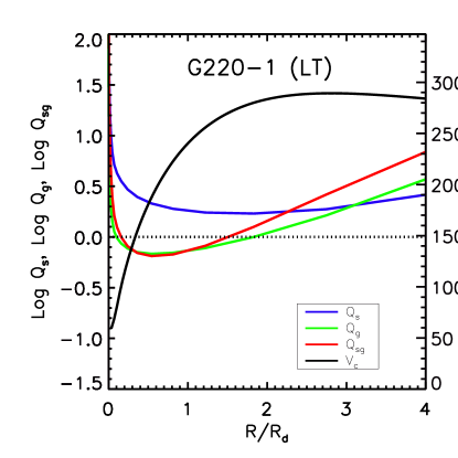
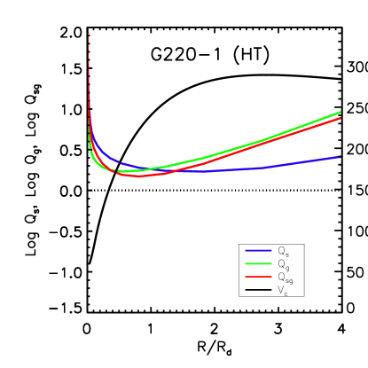
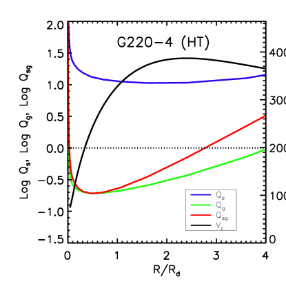
Figure 1: The initial gravitational instability and rotation curve of (top panels) low $T$ galaxy models G100-1 and G220-1 with different rotation velocities, and (bottom panels) high $T$ models G220-1 and G220-4 with different gas fractions. (Model parameters are given in Table 1.) Shown are the radial profiles of the instability parameters, $Q_{\rm s}$ for stars (blue), $Q_{\rm g}$ for gas (green), and $Q_{\rm sg}$ for stars and gas together (red), respectively. The black line is the curve of rotational velocity $V_{\rm c}$, with scale given on the right. $R_{\rm d}$ is the radial disk scale length, given in Table 1. The line of marginal stability $Q=1$ is also shown.

The isolated galaxy models in our simulations cover a wide range of total mass and gas fraction. The models with disk fraction $m_{\rm d}$ = 0.05 have flat rotation curves out to the virial radius, while in models with $m_{\rm d}$ = 0.10, the rotation curves drop slightly after a few disk scale lengths, as shown in Figure 1. This Figure also shows the radial profiles of the Toomre instability parameters for stars $Q_{\rm s}$, gas $Q_{\rm g}$, and the combination $Q_{\rm sg}$ for several selected models with different mass, sound speed, and disk gas fraction. They are calculated from equations (2)–(4) using the initial conditions, taking the most unstable wavenumber $k$ at each radius. Note that $Q_{\rm s}$ is shown, rather than Toomre’s Q for the stars, so a factor $3.36/\pi=1.07$ should be divided out when compared to commonly quoted $Q$ values (e.g. in Kennicutt 1989; Martin & Kennicutt 2001). Axisymmetric gravitational instability occurs when $Q<1$ (or, in the stellar case $Q_{\rm s}<1.07$).

All three Q-curves have a similar dependence on galactic radius, dropping to a minimum point at radius $R_{\rm min}$ and then rising. The stellar $Q_{\rm s}$ varies slowly, while in many galaxies $Q_{\rm g}$ and $Q_{\rm sg}$ vary more dramatically with radius. Comparison of the models with the same gas fraction but different total mass (top row) shows that the minimum value of $Q_{\rm g}$ and $Q_{\rm sg}$ decrease as galaxy mass increases, while the size of the unstable region where $Q_{\rm sg}<1$ increases with the mass of the galaxy. Comparison of the models with the same total mass but different gas fraction (bottom row) shows that the minimum values of $Q_{\rm g}$ and $Q_{\rm sg}$, decrease as gas fraction increases, while the size of the unstable area increases with gas fraction. Gas-rich, massive galaxies are more unstable than gas-poor, low-mass galaxies. The more unstable the galaxy, the smaller $R_{\rm min}/R_{\rm d}$ is. For example, G220-4 has $R_{\rm min}\approx$ 0.4 $R_{\rm d}$, while G100-1 has $R_{\rm min}\approx$ 1.4 $R_{\rm d}$. The size of the unstable regions range from $<2\ R_{\rm d}$ in small galaxies to $\approx 5\ R_{\rm d}$ in the most unstable galaxies.

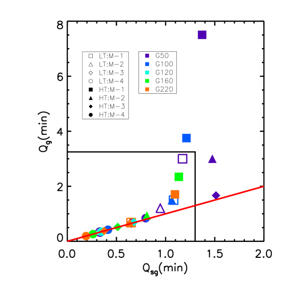
Figure 2: Comparison of minimum initial $Q_{\rm g}$ and $Q_{\rm sg}$ for both low $T$ (open symbols) and high $T$ (filled symbols) models described in Tables 2 and 3, as shown in the legend. Labels from M-1 to M-4 are submodels that indicate increasing gas fraction, as given in Table 1. The color of the symbol indicates the rotational velocity for each model. The red line indicates $Q_{\rm g}=Q_{\rm sg}$. The rectangle encloses galaxies that form stars in the first 3 Gyrs in the simulations.

The Toomre parameter typically measured is $Q_{\rm g}$ (e.g., Kennicutt 1998a), while instability is actually determined by $Q_{\rm sg}$. A comparison of the minimum initial $Q_{\rm g}(min)$ and $Q_{\rm sg}(min)$ for all our models is shown in Figure 2. When less than unity, $Q_{\rm g}(min)\approx Q_{\rm sg}(min)$, as shown also in Figure 1. For values above unity, though, $Q_{\rm g}(min)\gg Q_{\rm sg}(min)$. Insofar as our empirical initial conditions reproduce real galaxies, this suggests that $Q_{\rm g}$ and $Q_{\rm sg}$ are equivalent in strongly unstable galaxies, but in stable or marginally stable galaxies, $Q_{\rm g}$ alone may be insufficent to describe the stability of the system, because it does not take into account the destabilizing effect of the stellar disk mass. In small galaxies such as dwarfs, or in gas-poor galaxies, stars tend to be more important than gas in causing gravitational instability in disks. Both stars and gas may need to be measured to fully characterize gravitational instability in galactic disks.

Star formation is closely related to the value of $Q_{\rm sg}(min)$, as shown by the rectangle in Figure 2. The most unstable model in the sample, G220-4 (high T) with $Q_{\rm sg}(min)\approx 0.2$, has the most violent starburst, while the stable models outside the rectangle do not form any stars in the first 3 billion years. The critical value for star formation, $Q_{\rm sg}\approx 1.6$ will be derived with equation (7) in § 5 below. When $Q_{\rm sg}>1.6$, it is hard to form stars in a galaxy.

4 STAR FORMATION MORPHOLOGY

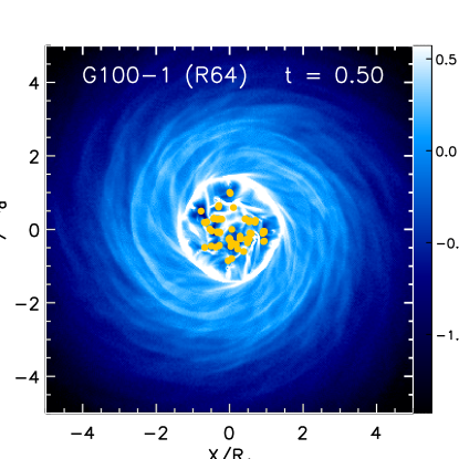
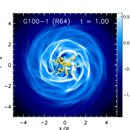
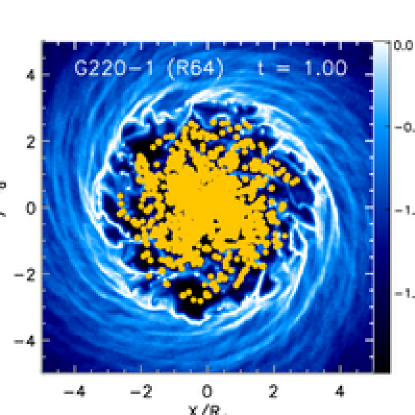
Figure 3: Star formation in the highest resolution (R64, with $N_{\rm tot}=6.4\times 10^{6}$) low $T$ models, with differing rotational velocities and total mass G100-1 (left column) and G220-1 (right column). The blue-white image shows atomic gas surface density as indicated by the color bars, while the yellow dots are sink particles representing both molecular gas and stars. Time $t$ is given in units of gigayears.

Figure 3 shows sink particle locations in several of our low T galaxy models, superposed on the atomic gas column density distribution. Again, keep in mind that sink particles represent regions of gravitational collapse that include both molecular gas and stars. To produce the gas column density image, the atomic gas density (SPH particles not accreted into sinks) is projected to the x-y plane and then smoothed with an adaptive kernel that always includes at least 32 gas particles. The columns in Figure 3 show time evolution while the rows show different models.

Figure 3 shows that spiral structure develops in each galaxy model, but it consists only of flocculent spiral arms (with numerous short arms), not grand design (with two long symmetric arms, such as M51), or multiple arm (with several long arms, such as our Milky Way) patterns. This suggests that gravitational instability does not cause isolated galaxies to form long spiral arms. We discuss this further in § 8. Gravitational collapse resulting in star formation occurs as the gas density increases in the spiral arms. Collapse occurs first in the higher density regions near the galactic center, and then extends over time to larger radii.

Star formation depends on the mass of the galaxy. Small galaxies such as G100-1 form stars slowly, while massive ones such as G220-1 have vigorous starbursts at early time. The size of the star-forming region relative to the scale of the galaxy increases with galaxy mass as well. For example, at $t=1$ Gyr, star clusters form only within $1\ R_{\rm d}$ in G100-1, but in G220-1, they form out to $3\ R_{\rm d}$.

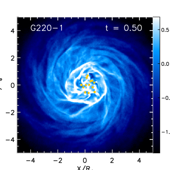
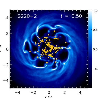
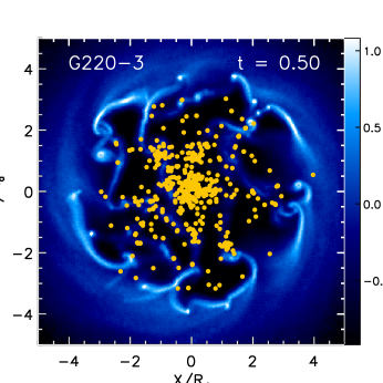
Figure 4: Same as Figure 3, but for high T models with the same total mass but different gas fractions, $f_{\rm g}$ = 0.2, 0.5, 0.9 of the disk mass for G220-1, 2, 3, respectively, and disk fraction $m_{\rm d}=0.05$ of the total mass.

Star formation also depends on the gas fraction of the galaxy disk. Figure 4 shows models at one time with the same total mass but different gas fractions. As the galaxy becomes more gas rich, collapse becomes more vigorous, and the relative size of the star formation region increases. The high density regions in the spiral arms collapse most quickly, aligning star formation with the arms. For example, at $t=0.5$ Gyr, clusters form within $1\ R_{\rm d}$ in G100-1, while in G100-4 they form out to 5 $R_{\rm d}$.

Taken together, Figures 3 and 4 illustrate that rapid, widespread star formation takes place in massive or gas-rich, unstable galaxies, while slow, centralized star formation occurs in more stable galaxies.

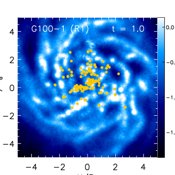
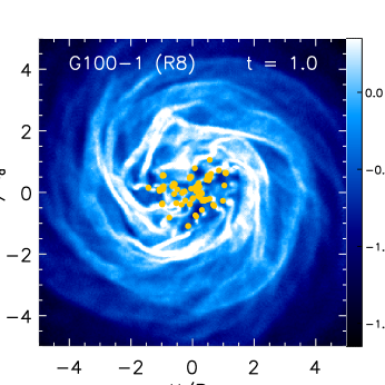
Figure 5: Gas surface density maps from the resolution study, showing versions of G100-1 (LT) with total particle number of $N_{\rm tot}=10^{5}$ (R1), $8\times 10^{5}$ (R8) and $6.4\times 10^{6}$ (R64). Model R1, which is underresolved according to the criterion of Bate & Burkert (1997), shows strong spurious fragmentation. On the other hand model R8, which is marginally resolved, shows only minor differences with the highest-resolution model R64, suggesting the criterion is adequate.

Figure 5 shows the maps of gas surface density from our resolution study of model G100-1. In the low resolution run R1 where the Bate & Burkert (1997) mass resolution criterion is not satisfied, strong spurious fragmentation occurs. However, models R8 and R64, which comply with the three criteria, look similar, and both look different from the first one. This suggests that the mass-resolution criterion of Bate & Burkert (1997) is adequate for our problem. We will confirm this by examination of resolution effects on several other diagnostics that we study below.

As galaxies become more strongly gravitationally unstable the number of clusters formed also increases (Figure 6). Unstable galaxies, with higher rotational velocites $V_{\rm c}$ or higher gas fractions (higher submodel numbers in most cases) produce more clusters than their more stable, small or gas poor counterparts. The low $T$ models are more unstable than their high $T$ counterparts, and they also produce more clusters for the same galactic parameters.

To check whether the cluster numbers shown in Figure 6 have numerically converged, we compare in Figure 7 the cluster number in the runs of the resolution study of models G100-1 and G220-1. Moving from run R1 to run R8, increasing linear resolution by a factor of two, shows a change by a factor of two in cluster number. However, further increase in resolution shows rather smaller variations of $\approx 30$%, but in random directions, suggesting that convergence effects are being overwhelmed by cosmic variance caused by chaotic dynamics (see discussion of Figure 6 in Klessen, Heitsch, & Mac Low 2000).

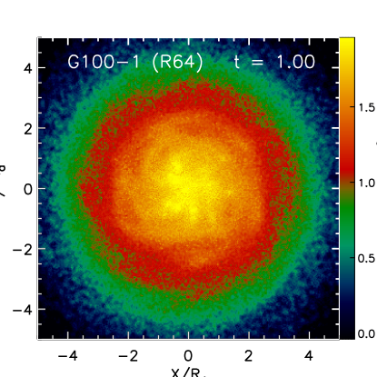
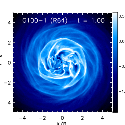
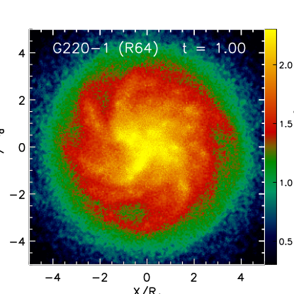
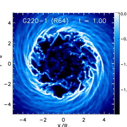
Figure 8: Comparison of the old stellar disk (left column) and the atomic gas disk (right column) of LT models G100-1 and G220-1 at $t=1$ Gyr. Both models have $N_{\rm tot}=6.4\times 10^{6}$. The images are the surface densities of stars and gas, respectively, as shown by the color bars. The sink particles, which represent both molecular gas and stars, are not included in these images.

The old stellar disk and the gas disk evolve differently. A comparison of the two is shown in Figure 8, showing their different morphologies. The stellar disk does not evolve much over time in any of our models, probably because of its lack of dissipation. In contrast, the gas disk evolves quickly, as seen in model G220-1. High density regions formed by gravitational instability collapse, turning atomic gas into molecular gas and stars, as represented by the sink particles (not shown in Fig. 8). The resulting disk has a gas distribution that is mostly atomic in the outer disk but molecule-dominated in the central region (better seen in Fig. 3), agreeing with observations by Wong & Blitz (2002).

5 STAR FORMATION HISTORY

Star formation occurs at different times in different galaxies. Some galaxies appear to have formed the bulk of their stars shortly after formation, while some, even after billions of years, are still forming stars (Kennicutt 1998a). Stars form at different times and with different global efficiencies in different model galaxies as well. Because we neglect both gas recycling and galaxy interactions, our models cannot represent the full star formation history of any real galaxy. Instead, they represent physics experiments that give the response of gravitational instability to the chosen initial conditions in each model. The results of these experiments do, however, appear very relevant to explaining the behavior of real galaxies.

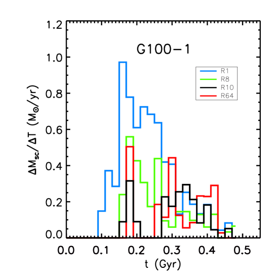
Figure 10: Same as Figure 9, but for resolution study of model G100-1 with R1 (blue), R8 (green), and R64 (red). The standard resolution of R10 is also shown (black).

Figure 9 shows the star formation history over the first 500 Myrs of representative models, measured by the mass of gas accreted into sink particles over periods of 20 Myr, multiplied by our assumed local SFE of 30%. This figure has the same arrangement as Figure 1. Comparison of models with the same gas fraction but different total mass, and models with the same total mass but different gas fraction, illustrates that the star formation timescale and the mass of gas turned into stars depend strongly on the total mass and the gas fraction of the galaxy. Stars form early and efficiently in unstable galaxies, in contrast to late and slow formation in more stable ones. Figure 10 demonstrates that failing to resolve the Jeans length can lead to a factor of two overestimate in the star formation rate, as can be seen by comparison of R1 to the higher resolutions. Once the Jeans length is resolved, the time history is generally well converged, although details vary between models with different resolution.

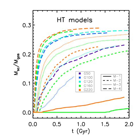
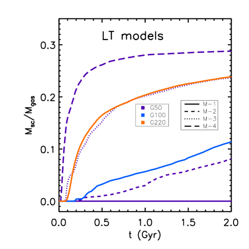
Figure 11: Time history of the mass in star clusters $M_{\rm sc}$ in all (a) high $T$ and (b) low $T$ galaxy models in Table 2 and 3, scaled by initial total gas mass $M_{\rm gas}$. Again $M_{\rm sc}$ is taken as 30% of the mass of the sink particles. M-1 to 4 indicate submodels with increasing gas fractions, as given in Table 1.

Figure 11 shows integrated time histories of star formation normalized by the initial total gas mass $M_{\rm sc}(t)/M_{\rm gas}$. (Note that the global SFE can never exceed our assumed local SFE of 30%.) These histories reflect the same dependence on stability as the differential histories shown in Figure 9. Fast star formation occurs early and goes on until all the gas has collapsed into sink particles after a few hundred megayears, while slow star formation occurs late and tends to last over many gigayears.

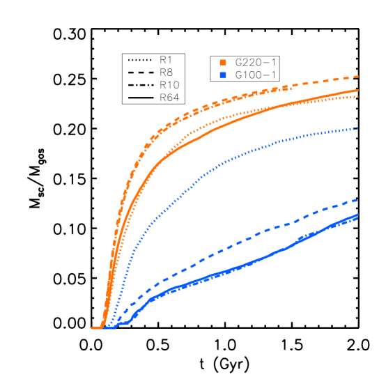
Figure 12: Same as Figure 11 but for resolution study of models G100-1 and G220-1, with resolution levels of R1 (dotted line), R8 (dashed line), and R64 (solid line). The standard resolution R10 model is also shown (dash-dotted line).

In agreement with Figure 9, Figure 12 shows that spurious fragmentation can dominate the accreted mass (multiplied in the Figures by our assumed SFE) in our low-resolution model R1, but that the accreted mass has converged to within 10% in model R8 as compared to model R64. The integrated mass converges better than the differential mass shown in Figure 10, suggesting that the variations seen there reveal fluctuations in a process that produces a more stable average behavior. Both models of G100-1 and G220-1 show convergence of the integrated mass accreted in runs that satisfy the three numerical criteria, suggesting that our standard criteria are sufficient for the problem studied here.

The mass curves in Figure 11 appear to have a functional behavior of the form

$$\frac{M_{\rm sc}}{M_{\rm gas}}=M_{0}\left[1-\exp(-t/\tau_{\rm SF})\right]\,,$$ (4)

where $M_{0}$ is the maximum fraction of initial total gas turned into star clusters, and $\tau_{\rm SF}$ is the star formation timescale. Again, bear in mind that this is a description of the physical response of a galactic disk to the initial conditions for each model, not a description of the star formation history of a real galaxy interacting with its cosmic environment.

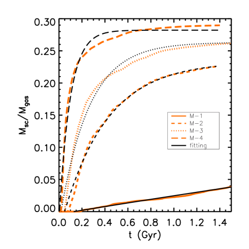
b

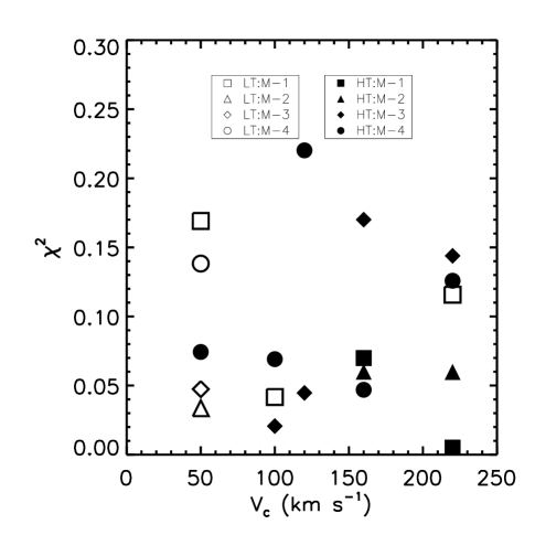
Figure 13: Same as Figure 11 but with fits to equation (4). a: Examples of fits to high $T$ model G220. b: The relative goodness of the fits indicated by $\chi^{2}$, as defined in the text.

Figure 13(a) demonstrates that equation 4 fits models of G220 rather well. Figure 13(b) shows the statistical relative goodness of the fits, indicated by the parameter $\chi^{2}=\sum(y_{i}-y_{f})^{2}$, where $y_{i}$ are points drawn from the simulation history, while $y_{f}$ are analytic values from the best-fit parameters in equation (4).

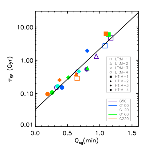
b

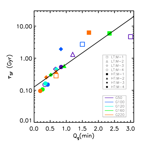
Figure 14: Star formation timescale $\tau_{\rm SF}$ correlates with the initial disk instability (a) $Q_{\rm sg}$ (from Li et al. 2005) and (b) $Q_{\rm g}$ for both low $T$ (open symbols) and high $T$ (filled symbols) models. The solid lines are least-squares fits to the data.

The star formation timescale $\tau_{\rm SF}$ appears to be closely correlated with the minimum initial values of the gravitational instability parameters $Q_{\rm g}(min)$ and $Q_{\rm sg}(min)$ (Li et al. 2005). Figure 14 shows the relations between $\tau_{\rm SF}$ and $Q_{\rm sg}(min)$ and $Q_{\rm g}(min)$ for all high-resolution models. An exponential function describes both relations rather well, with the correlation being rather better to $Q_{\rm sg}(min)$ than to $Q_{\rm g}(min)$. The best fits are

$$\tau_{\rm SF} = \left(34\pm 7\mbox{Myr}\right)\exp\left[Q_{\rm sg}(min)/0.24\right],$$ (5)

$$\tau_{\rm SF} = \left(127\pm 9\mbox{Myr}\right)\exp\left[Q_{\rm g}(min)/0.61\right].$$ (6)

In stable galaxies with large $Q_{\rm sg}$, $\tau_{\rm SF}$ is large, and stars form slowly over a long time. They resemble normal disk galaxies. In unstable galaxies with small $Q_{\rm sg}$, $\tau_{\rm SF}$ is small, and vigorous star formation occurs until the gas is used up or the galaxy is stabilized again. They resemble starburst galaxies. Typical observed starburst times of order $10^{8}$ yr are consistent with our fits for $\tau_{\rm SF}$ in unstable galaxies (Kennicutt 1998a).

For a Milky Way-size disk model, $M_{\rm 200}\approx 1.3\times 10^{12}\ M_{\odot}$, $m_{\rm d}\approx 6\%$ , and $f_{\rm g}\approx 7\%$ (Dubinski et al. 1996; Dehnen & Binney 1998; Widrow & Dubinski 2005), the calculated minimum initial Toomre Q parameter of $Q_{\rm sg}(min)\approx 1.2$ with effective sound speed $c_{\rm s}=6$ km s^-1. The predicted star formation timescale according to Figure 14 is around 5.2 Gyrs. If a bulge with mass of $\sim 10^{10}M_{\odot}$ and size of $\sim 2$ kpc is included in the model, the resulting minimum initial $Q_{\rm sg}(min)\approx 1.23$, which gives $\tau_{\rm SF}\simeq 6$ Gyrs, agreeing well with observations.

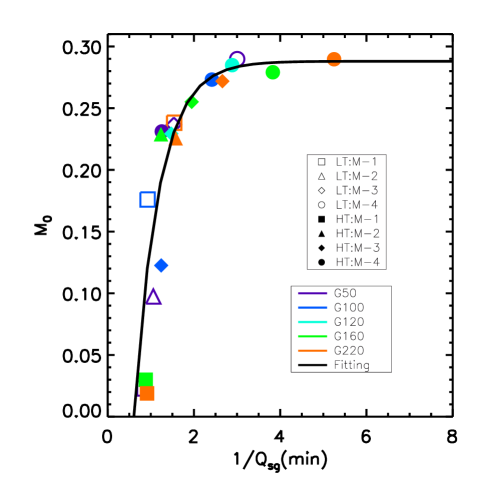
b

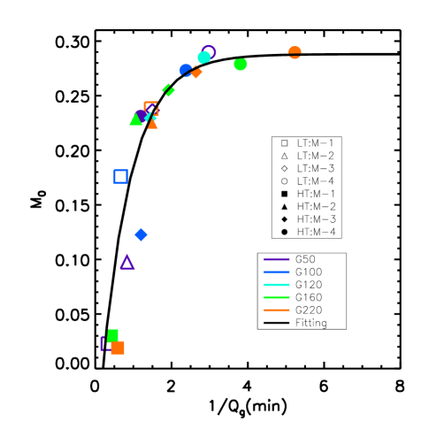
Figure 15: The maximum fraction $M_{0}$ of gas accreted onto clusters as a function of (a) $Q_{\rm sg}(min)$ and (b) $Q_{\rm g}(min)$. Solid lines indicate best fits of the form given in equation (7).

Figure 15 shows the final fraction of total gas formed into stars $M_{0}$ as a function of the minimum initial instability parameters $Q_{\rm sg}(min)$ and $Q_{\rm g}(min)$. The solid line is the best fit to both the low $T$ and high $T$ models, which gives:

$$M_{0} = 0.29\{1-2.88\exp\left[-1.74/Q_{\rm sg}(min)\right]\},$$ (7)

$$M_{0} = 0.29\{1-1.28\exp\left[-1.28/Q_{\rm g}(min)\right]\}\,.$$ (8)

(Note that our assumption of a local SFE of 30% gives an upper limit to $M_{0}$ of 0.3.) In order for a galaxy to form stars, $M_{0}$ should be positive. This gives the empirical constraints $Q_{\rm sg}<1.6$ and $Q_{\rm g}<5.2$.

6 RADIAL AND VERTICAL DISTRIBUTIONS

Figure 16 shows the radial distribution of gravitational collapse and star formation in different low $T$ models. The arrangement of the panels is the same as in Figure 1 for direct comparison. Star formation takes place in the unstable regions outlined by the Q-curves in Figure 1.

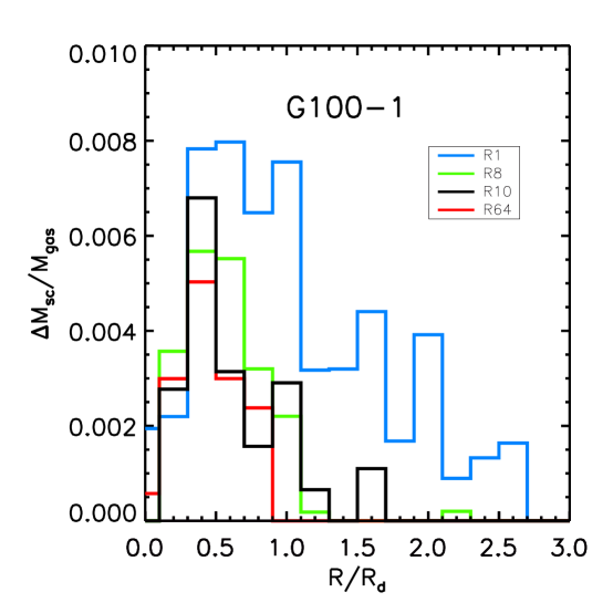
Figure 17: Same as Figure 16 but for resolution study of model G100-1, with R1 (blue), R8 (green), and R64 (red). The standard resolution R10 is also shown (black).

The most unstable radius, where $Q_{\rm sg}$ reaches a minimum, coincides with the radial peak of star formation in most models. The normalized size of the star formation region $R_{\rm SF}$ increases with the mass, or the gas fraction of the galaxy. For example, $R_{\rm SF}\approx$ 2 $R_{\rm d}$ in G100-1, but expands to $\approx$ 5 $R_{\rm d}$ in G220-4. Figure 17 shows that the underresolved R1 model produces too much star formation at most radii, but that for the standard resolution R10 model the radial distribution of clusters has converged quite well.

Figure 18 shows the vertical distribution of collapse and star formation in the same models as in Figure 16. The bin size of the histogram is $0.1H_{\rm d}$, where the vertical disk scale length of the stars $H_{\rm d}=0.2\ R_{\rm d}$ as set up in the models. The vertical thickness of the star forming region also depends on the mass and gas fraction of the galaxy. In small, or gas-poor galaxies, stars form in a wide spatial distribution along the vertical direction ($Z\approx 1\ H_{\rm d}$). As the galaxy becomes more unstable, star formation becomes more vigorous and is more concentrated in a narrow range in the galactic plane ($Z<0.3\ H_{\rm d}$).

Both Figures 16 and 18 illustrate that the spatial distribution of star formation in isolated disk galaxies depends on the gravitational stability of the galaxy. In unstable galaxies, most of the gas turns into stars quickly. The star formation regions reach several disk scale lengths, but vertically they concentrate in the galactic plane. In more stable galaxies, only a small fraction of the gas forms stars, over a long period. The star formation region is radially concentrated in the central region but vertically extended out of the galactic plane.

The correlation is quantified in Figure 19, which shows that the normalized vertical scale height of star clusters, $H_{\rm sc}/H_{\rm d}$ increases linearly with the minimum initial disk instability $Q_{\rm sg}(min)$. $H_{\rm sc}$ is calculated from the variance of the vertical distribution of the star clusters. Regions of gravitational collapse will form molecular clouds with high extinction in addition to stellar clusters. The distribution of sink particles thus also roughly traces the distribution of molecular gas, as briefly discussed by Li et al. (2005). Our result that unstable galaxies have smaller $H_{\rm sc}$ than stable galaxies thus implies that they also have thinner dust lanes. This result agrees well with the observations by Dalcanton et al. (2004), who find that thin dust lanes only form in nearby galaxies with $V_{\rm c}\geq 120$ km s^-1. They find that gas-poor modern galaxies are typically Toomre unstable using the Rafikov (2001) criterion when $V_{\rm c}\geq$ 120 km s^-1.

7 CORRELATED STAR FORMATION

Observations of star clusters in the Large Magellanic Cloud have shown that there is a correlation between spatial separation $\Delta S$ and age difference $\Delta T$. Efremov & Elmegreen (1998) show that $\log\Delta T\sim 0.35\log\Delta S$, and argue that this correlation is due to the hierarchical structure of turbulence (see also Nomura & Kamaya 2001).

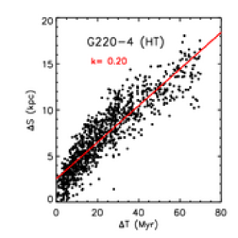
Figure 20: Linear correlation between separations of cluster pairs $\Delta S$ and their age differences $\Delta T$ in models G100-4, G160-4, and G220-4 at model times equal to their characteristic star formation timescales $\tau_{\rm SF}$. The clusters shown here have age 10 Myr $<T<100$ Myr. The red lines represent least squares fits, with slopes $k$ given in each panel.

Figure 3 shows that the distribution of star clusters in our models also appears structured rather than smooth. Figure 20 shows that for any random reference cluster, the separation $\Delta S$ of the cluster pairs is linearly correlated to their relative age $\Delta T$. Neighboring clusters tend to form coevally, while distant pairs tend to form at different times. This behavior is seen in all of our models.

For comparison with our models, the data used by Efremov & Elmegreen (1998) is replotted on a linear scale in Figure 21. Their $\Delta S$ is converted from degrees to kpc in the original plots (Figure 1 of Efremov & Elmegreen 1998), by using the mean distance to the Large Magellanic Cloud of 45 kpc given in the same paper. Only data with $\Delta S\leq 1^{\circ}$ (corresponding to 0.78 kpc) is plotted here to maintain consistency with the original fits. We see that this data can be well fit by a linear correlation, similarly to our model results.

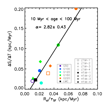
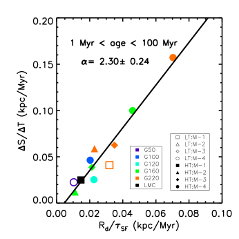
Figure 22: The correlation between $\Delta S/\Delta T$ and the galaxy properties $R_{\rm d}/\tau_{\rm SF}$, for clusters with different ages $T$ in all models. a: For 10 Myr $<T<100$ Myr, b: for 1 Myr $<T<100$ Myr, and c: for 1 Myr $<T<1000$ Myr. The black line is the least-square fit to the data, while the black square represents the fits shown in Figure 21 to the observed star clusters in the Large Magellanic Cloud from Efremov & Elmegreen (1998).

Our models suggest that a linear $\Delta S$–$\Delta T$ correlation is the natural result of gravitational collapse in a differentially rotating disk. It occurs for all ages of clusters in all of our models, as is demonstrated in Figure 22. This Figure further shows that the linear slope of the $\Delta S$–$\Delta T$ relation is directly proportional to the star formation rate $\tau_{\rm SF}^{-1}$ derived in §5 multiplied by the disk scale length $R_{\rm d}/\tau_{\rm SF}$. The stronger the instability, the more frequently clusters form, and so the greater distance $\Delta S$ one must traverse to find clusters with a given age difference $\Delta T$.

The Large Magellanic Cloud has a halo mass of $M_{\rm halo}\approx 1.6\times 10^{10}M_{\odot}$, gas mass $M_{\rm gas}\approx 1\times 10^{9}M_{\odot}$, and radial disk scale length $R_{\rm d}=1.47$ kpc (van der Marel 2001; Alves 2004). It is close to our model G50-4, so we estimate it to have a comparable star formation timescale $\tau_{\rm SF}$ for the current episode of $\sim 100$ Myr. With this estimate, our fits to the data drawn from Efremov & Elmegreen (1998) fall on the correlation derived from our models strikingly well, as shown in Figure 22. (Note that even a substantially larger value of $\tau_{\rm SF}$ would not markedly change this conclusion.)

These correlations survive among clusters as old as 1 Gyr, as shown in Figure 22(c). This suggests that the observed $\Delta S$–$\Delta T$ correlation is simply the result of gravitational interaction. Interstellar turbulence in the galactic disk cannot determine cluster positions as long as 1 Gyr after cluster formation. The mixing time—the generalization to supersonic flow of the eddy turn-over time—is an order of magnitude shorter (de Avillez& Mac Low 2002; Klessen & Lin 2003), so turbulent structures will be uncorrelated on those timescales.

Unstable galaxies have a high slope of $\Delta S$ versus $\Delta T$, which appears to imply fast star formation, while more stable galaxies have slower star formation and smaller slopes.

8 DISCUSSION

The simulations presented here model the nonlinear development of gravitational instability in isolated galaxies. They represent the response of the galactic disks to the initial conditions imposed in each case, but do not directly represent the star-formation history of real galaxies interacting with their environment. Nevertheless, we think our models yield useful insights into the behavior of real galactic disks. Furthermore, in the simulations presented here, we do not include explicit feedback, magnetic fields, or gas recycling from star-forming regions, all of which will affect the detailed star formation history and gas evolution, so they will eventually have to be considered. However, we believe each will have minor effects on the questions considered here, for reasons that we now describe.

The assumption of an isothermal equation of state for the gas actually implies substantial feedback to maintain the effective temperature of the gas against radiative cooling and turbulent dissipation. Real interstellar gas has a wide range of temperatures. However, the rms velocity dispersion generally falls within the range 6–12 km s^-1 (e.g., Scalo & Elmegreen 2004). Direct feedback from the starburst may play only a minor role in quenching subsequent star formation (e.g. Kravtsov 2003; Monaco 2004), perhaps because most energy is deposited not in the disk but above it as superbubbles blow out (e.g. Fujita et al. 2003; de Avillez & Breitschwerdt 2004). At least three effects may conspire to maintain the velocity dispersion in the observed narrow range. First, radiative cooling drops precipitously in gas with sound speed $\lesssim$ 10 km s^-1 as it becomes increasingly difficult to excite the Lyman $\alpha$ line of hydrogen. Second, the energy input $\dot{E}$ from supernovae at the observed Galactic rate drives a flow with rms velocity dispersion of $\sim$ 9.5 km s^-1 (de Avillez 2000), and the rms velocity dispersion depends only on $\dot{E}^{1/3}$ (Mac Low 1999; Mac Low & Klessen 2004), so a wide range of star formation rates leads to a narrow range of velocity dispersions. Third, magnetorotational instabilities may maintain a velocity dispersion of order 6 km s^-1 even in the absence of any other feedback (Sellwood & Balbus 1999; Dziourkevitch, Elstner, & Rüdiger 2004).

Kim & Ostriker (2001) have demonstrated that swing and magneto-Jeans instabilities operating in a gaseous disk occur at a Toomre instability criterion of $Q_{\rm g}\approx 1.4$, suggesting that magnetostatic support is unimportant. Another longstanding question is how fragmentation can proceed in the presence of a magnetic field. Material collects from considerable distance in our models. If it is constrained to flow along field lines, collapse can still occur in so long as the mass-to-flux ratio remains supercritical along each field line. So long as the local mass-to-flux ratio remains supercritical, the magnatic field can retard the contraction but not prevent it (Heitsch et al. 2001; Vázquez-Semadeni et al. 2004).

In our simulations, we do not include any gas recycling so that sink particles form until the gas is consumed. However, in reality there are at least three sources of gas that ultimately need to be taken into account. First, in our picture, the bulk of the cold, molecular gas, which is primarily contained in giant molecular clouds, is already gravitationally unstable and either forming stars or being dispersed on a free-fall time (Hartmann, Ballesteros-Paredes, & Bergin 2001). Some fraction of that dispersed mass may rejoin the diffuse, gravitationally stable gas, while the rest will participate within tens of megayears in further star formation not taken into account by our assumed SFE. Second, the massive stars in newly-formed clusters evolve quickly, and at the end of their lives eject part of their mass back into the interstellar gas, supplying a gas reservoir for the next cycle of star formation until all the mass is locked up in low mass stars or compact objects. Finally, galaxies are not isolated objects, but accrete further mass from interactions and the intergalactic medium. Our models do not take this into account, but form the basis for models that do. For a first example, see Li, Mac Low, & Klessen (2004).

There have been many models of the formation of spiral structure (e.g., Lin & Shu 1966; Roberts 1969; Toomre 1977; Sellwood & Carlberg 1984; Binney & Tremaine 1987; Elmegreen, Elmegreen, & Leitner 2003) that offer a general picture that spiral structure is a combination of sheared features from star formation and density waves in the gas and stars. The wide variety of spiral structure observed in different galaxies is due to the wide range of the swing amplifier that depends on the response of the galactic disk to the perturbation from gravitational instability, tidal forces, or bar formation. Grand-design spiral structures are usually thought to be produced by perturbations or interactions (e.g., Kormendy & Norman 1979), as seen also in our simulations of galaxy mergers using models similar to the ones described here (Li et al. 2004).

Elmegreen & Thomasson (1993) showed grand design spiral arms forming in isolated galaxies in 2D simulations with resolutions from 42 $\times$ 64 to 84 $\times$ 128 grid cells. However, their models assume a very large disk mass fraction $m_{\rm d}$ = 0.2, so that the rotation curve falls sharply at large radii, rather than remaining constant as is typically observed. Moreover, their model uses a very cold disk with a hot stellar population in the central part to produce a Q-barrier. This produces a highly unstable disk that forms stars in a violent starburst. Their simulations using galaxy models having parameters more typical of normal spirals, and without the Q-barrier, show flocculent features only. Furthermore, their inability to resolve the Jeans length probably induces spurious fragmentation and artificial spiral arms (Truelove et al. 1997), as we demonstrated in Figure 5. Our 3D simulations with high resolution, and more realistic galaxy models with $m_{\rm d}\leq 0.1$ and flat rotation curves (shown in Figure 1) show clear flocculent arms. Elmegreen et al. (2003) proposed a turbulent origin for flocculent spiral arms, but our results suggest that gravitational instability in the absence of external perturbations can fully explain them.

Our resolution study demonstrates that the gas density distribution, the number of fragments and the collapsed mass converge sufficiently well when $N_{\rm k}\geq 2$, supporting the validity of the numerical criteria used in our simulations. Simulations of isolated, isothermal disks by Robertson et al. (2004) show large-scale collapse in the galactic center leading to disks far smaller than observed, which they argued was caused by the isothermal equation of state. Our model G100-1 has parameters close to theirs but with an order of magnitude higher particle number that resolves the Jeans length as suggested by the Bate & Burkert (1997) criterion. It does not show this behavior. Similarly, Governato et al. (2004) argue that several long-standing problems in galaxy simulations, such as compact disks, overly efficient star formation, and lack of angular momentum may well be caused by inadequate resolution, or violation of the other numerical criteria.

9 SUMMARY

To summarize our work, we have simulated star formation with sufficient resolution to resolve gravitational collapse in models ofa wide range of disk galaxies with different total mass, gas fraction, and initial gravitational instability.

The gravitational collapse or star formation timescale $\tau_{\rm SF}$ depends exponentially on the initial Toomre instability parameter for the combination of stars and gas in the disk $Q_{\rm sg}$ given by Rafikov (2001). The tight correlation between $\tau_{\rm SF}$ and $Q_{\rm sg}(min)$ suggests that the global star formation rate in isolated disk galaxies is controlled by the nonlinear development of gravitational instability. Quiescent star formation occurs where $Q_{\rm sg}$ is large, while vigorous starbursts occur where $Q_{\rm sg}$ is small. Star formation begins when the gas become unstable, with a rate controlled by $Q_{\rm sg}(min)$. Galaxies with high initial mass or gas fraction are the most unstable, forming stars quickly. The number of star clusters formed also appears to depend on the strength of instability.

Our models show that stars form in gravitationally unstable regions as defined by $Q_{\rm sg}$. The star formation region in strongly unstable galaxies extends multiple disk scale lengths in radius, but is concentrated to less than a tenth of a scale height vertically, while in marginally unstable galaxies it concentrates radially in the central scale length, but extends for more than half a scale height vertically. These results directly agree with the observations of Dalcanton et al. (2004) that unstable galaxies show thin dust lanes, while more stable galaxies show thick dust distributions.

Star clusters do not form uniformly but rather are distributed so that their spatial separation $\Delta S$ and age difference $\Delta T$ correlate linearly with each other. The slope of the correlation depends directly on the star formation rate multiplied by the disk scale length $R_{\rm d}/\tau_{\rm SF}$. Observations of Large Magellanic Cloud clusters by Efremov & Elmegreen (1998) quantitatively agree with this dependence.

In future work we will study global and local Schmidt laws, star formation thresholds, and the mass distribution of the clusters that form in our models.

Table 1: Galaxy Models

Model	$V_{200}$	$R_{200}$	$M_{200}$	$m_{\rm d}$	$f_{\rm g}$	$R_{\rm d}$
G50-1	50.0	71.43	4.15	0.05	0.2	1.41
G50-2	50.0	71.43	4.15	0.05	0.5	1.41
G50-3	50.0	71.43	4.15	0.05	0.9	1.41
G50-4	50.0	71.43	4.15	0.10	0.9	1.07
G100-1	100.0	142.86	33.22	0.05	0.2	2.81
G100-2	100.0	142.86	33.22	0.05	0.5	2.81
G100-3	100.0	142.86	33.22	0.05	0.9	2.81
G100-4	100.0	142.86	33.22	0.10	0.9	2.14
G120-3	120.0	171.43	57.4	0.05	0.9	3.38
G120-4	120.0	171.43	57.4	0.10	0.9	2.57
G160-1	160.0 6	228.57	136.0	0.05	0.2	4.51
G160-2	160.0 6	228.57	136.0	0.05	0.5	4.51
G160-3	160.0 6	228.57	136.0	0.05	0.9	4.51
G160-4	160.0 6	228.57	136.0	0.10	0.9	3.42
G220-1	220.0 0	314.29	353.7	0.05	0.2	6.20
G220-2	220.0 0	314.29	353.7	0.05	0.5	6.20
G220-3	220.0 0	314.29	353.7	0.05	0.9	6.20
G220-4	220.0 0	314.29	353.7	0.10	0.9	4.71

Table 2: Numerical Parameters for High Temperature Models

Model	$N_{\rm tot}$	$\epsilon_{\rm g}$	$m_{\rm g}$	$Q_{\rm sg}$(HT)	$N_{\rm k}$(HT)
G50-1	1.0	10	0.08	1.45	465.8
G50-2	1.0	10	0.21	1.53	177.8
G50-3	1.0	10	0.37	1.52	100.7
G50-4	1.0	10	0.75	0.82	49.7
G100-1	1.0	10	0.66	1.27	56.5
G100-2	1.0	10	1.65	1.07	22.6
G100-3	1.0	10	2.97	0.82	12.5
G100-4	1.0	20	5.94	0.42	6.3
G120-3	1.0	20	5.17	0.68	7.2
G120-4	1.0	30	10.3	0.35	3.6
G160-1	1.0	20	2.72	1.34	13.7
G160-2	1.0	20	6.80	0.89	5.5
G160-3	1.0	30	12.2	0.52	3.1
G160-4	1.5	40	16.3	0.26	2.3
G220-1	1.0	20	7.07	1.11	5.3
G220-2	1.2	30	14.8	0.66	2.5
G220-3	2.0	40	15.9	0.38	2.3
G220-4	4.0	40	16.0	0.19	2.3

Table 3: Numerical Parameters for Low Temperature Models

Model	$N_{\rm tot}$	$\epsilon_{\rm g}$	$m_{\rm g}$	$Q_{\rm sg}$(LT)	$N_{\rm k}$(LT)
G50-1	1.0	10	0.08	1.22	29.8
G50-2	1.0	10	0.21	0.94	11.4
G50-3	1.0	10	0.37	0.65	6.4
G50-4	1.0	10	0.75	0.33	3.2
G100-1	6.4	7	0.66	1.08	24.0
G220-1	6.4	15	7.07	0.65	2.3

Table 4: Resolution Study

$N_{\rm k}$	G100-1	G220-1
R1	0.38	0.035
R8	3.0	0.28
R64	24.0	2.3

Figure 6: Number of stellar clusters (sink particles) formed after 3 Gyr in both low $T$ (open symbols) and high $T$ (filled symbols) models, with properties given in Tables 1–3. Again M-1 to 4 indicate submodels that reflect different gas fractions, as given in Table 1.

Figure 7: Same as Figure 6 but for models of G100-1 (circles) and G220-1 (triangles) with different resolutions, as indicated by the total number of particles $N_{\rm tot}$.

Figure 9: Star formation histories for top panels) low $T$ galaxy models G100-1 and G220-1 with different rotation velocities, and (bottom panels) high $T$ models G220-1 and G220-4 with different gas fractions. $\Delta M_{\rm sc}$ is the mass collapsed into star clusters in a time interval of $\Delta T=$ 20 Myrs (the bin size). The mass of star clusters is taken as 30% of the mass of the sink particles as explained in the text.

a

a

a

Figure 16: Radial distribution of mass in star clusters $\Delta M_{\rm sc}$ in a bin size of 0.2 $R_{\rm d}$, normalized to initial gas mass $M_{\rm gas}$ after 3 Gyrs for (top panels) low $T$ galaxy models G100-1 and G220-1 with different rotation velocities, and (bottom panels) high $T$ models G220-1 and G220-4 with different gas fractions.

Figure 18: Vertical distribution of mass in star clusters $\Delta M_{\rm sc}$ in a bin size of $0.1H_{\rm d}$, normalized to initial gas mass $M_{\rm gas}$ after 3 Gyrs for (top panels) low $T$ galaxy models G100-1 and G220-1 with different rotation velocities, and (bottom panels) high $T$ models G220-1 and G220-4 with different gas fractions. The distance from the plane $Z$ is normalized by the vertical disk scale length $H_{\rm d}$.

Figure 19: Vertical scale height of star clusters formed within 3 Gyrs normalized by the vertical disk scale length, $H_{\rm sc}/H_{\rm d}$, correlates with the initial disk instability $Q_{\rm sg}(min)$.

Figure 21: Linear correlation between separations of cluster pairs $\Delta S$ in the Large Magellanic Cloud and their age differences $\Delta T$, reproduced from Efremov & Elmegreen (1998). a: For 1 Myr $<T<100$ Myr, b: for 10 Myr $<T<100$ Myr, and c: for 1 Myr $<T<1000$ Myr. Only data with $\Delta S\leq 0.78$ kpc, corresponding to $1^{\circ}$ (and indicated by the dotted line), is plotted here to maintain consistency with the original fits.

References

- Alves (2004) Alves, D. R. 2004, ApJ, 601, L151
- Barnes & Hut (1986) Barnes, J., & Hut, P. 1986, Nature, 324, 446
- Barnes (2002) Barnes, J. E. 2002, MNRAS, 333, 481
- Barnes & Hernquist (1996) Barnes, J. E., & Hernquist, L. 1996, ApJ, 471, 115
- Bate et al. (1995) Bate, M. R., Bonnell, I. A., & Price, N. M. 1995, MNRAS, 277, 362
- Bate & Burkert (1997) Bate, M. R., & Burkert, A. 1997, MNRAS, 288, 1060
- Ballesteros-Paredes et al. (1999) Ballesteros-Paredes, J., Hartmann, L., & Vázquez-Semadeni, E. 1999, ApJ, 527, 285
- Binney & Tremaine (1987) Binney, J., & Tremaine, S. 1987, Galactic Dynamics (Princetron University Press, Princeton)
- Boss & Bodenheimer (1979) Boss, A. P., & Bodenheimer, P. 1979, ApJ, 234, 289
- Dalcanton et al. (2004) Dalcanton, J. J., Yoachim, P., & Bernstein, R. A. 2004, ApJ, 608, 189
- de Avillez (2000) de Avillez, M. A. 2000, MNRAS, 315, 479
- de Avillez & Breitschwerdt (2004) de Avillez, M. A., & Breitschwerdt, D. 2004, A&A, 425, 899
- de Avillez& Mac Low (2002) de Avillez, M. A. & Mac Low, M. 2002, ApJ, 581, 1047
- Dehnen & Binney (1998) Dehnen, W. & Binney, J. 1998, MNRAS, 298, 387
- Dubinski (1996) Dubinski, J. 1996, New Astron., 1, 133
- Dubinski et al. (1996) Dubinski, J., Mihos, J. C. & Hernquist, L. 1996, ApJ, 462, 576
- Dziourkevitch et al. (2004) Dziourkevitch, N., Elstner, D., & Rüdiger, G. 2004, A&A, 423, L29
- Efremov & Elmegreen (1998) Efremov, Y. N., & Elmegreen, B. G. 1998, MNRAS, 299, 588
- Elmegreen (2002) Elmegreen, B. G. 2002, ApJ, 577, 206
- Elmegreen et al. (2003) Elmegreen, B. G., Elmegreen, D. M., & Leitner, S. N. 2003, ApJ, 590, 271