Nonhelical turbulent dynamos: shocks and shear

Abstract

Small scale turbulent dynamo action in compressible transonic turbulence is discussed. It is shown that the critical value of the magnetic Reynolds number displays a bimodal behavior and changes from a typical value of 35 for small Mach numbers to about 80 for larger Mach numbers. The transition between the two regimes is relatively sharp. The direct simulations are then compared with simulations where shocks are captured using a shock viscosity that becomes large at locations where there are shocks. In the presence of shear it is shown that large scale dynamo action is possible.

1 Introduction

There are two main classes of dynamos, small scale and large scale dynamos. This distinction is not completely unambiguous because in the presence of shear any small scale field will attain a large scale component in the direction of the shear. Therefore, the class of small scale dynamos is here confined to the case of nonhelical, isotropic and homogeneous turbulent flows (§2). With shear, however, even nonhelical dynamos can produce large scale fields (§3).

Members of the large scale dynamo class include turbulent flows with sufficient amounts of helicity and/or shear such that a large scale field is generated. Here, a large scale field is the component that survives after averaging. The averaging procedure has to be defined appropriately and depends on circumstances and also on what kind of field is generated. In the presence of a shear flow, ${\bm{U}}_{0}(x,z)=(0,U_{0},0)$, for example, a useful average (denoted by an overbar) will be

$$\overline{\bm{B}}={1\over L_{y}}\int_{0}^{L_{x}}{\bm{B}}\,{\rm d}{}y.$$ (1)

This definition will obviously preclude the study of nonaxisymmetric fields. In the case of helical turbulence, we have essentially an $\alpha$ effect, i.e. the turbulent electromotive force has a field-aligned component and $\overline{{\bm{u}}\times{\bm{b}}}\cdot\overline{\bm{B}}\neq 0$. Here, ${\bm{b}}={\bm{B}}-\overline{\bm{B}}$ is the fluctuating magnetic field and ${\bm{u}}={\bm{U}}-\overline{\bm{U}}$ is the fluctuating velocity. In unbounded space, for example, the mean field can have any orientation. Even in a triply-periodic domain there are still three ultimate field configurations, corresponding to Beltrami waves with variation in any of the three coordinate directions. The appropriate mean field is then best defined as a two-dimensional average over the other two coordinate directions.

Ideally, when defining averages we want to conform with the Reynolds rules (e.g. Krause & Rädler 1980). In particular, we want to make sure that the average of an average gives the same average (which is not the case for a running mean), and that average and derivative operators commute (not the case for averages over non-periodic directions, including time averages). We also want the average of a product of fluctuating and mean quantities to vanish (which is not the case for spectral filtering). Therefore, for many practical purposes, equation (1) is the preferred choice, avoiding any of the aforementioned problems.

A more formal characteristics of a successful large scale dynamo is therefore one where the ratio

$$q\equiv\langle\overline{\bm{B}}^{2}\rangle/\langle{\bm{B}}^{2}\rangle\gg R_{\rm m}^{-1}.$$ (2)

Here, angular brackets denote volume averages. Values of $q$ around 0.7 are typical under ideal conditions (see §3). Spiral galaxies tend to have $q\geq 0.2$ (e.g. Beck et al. 1996). For the sun the value of $q$ is unclear, but we would still classify it as a large scale dynamo even if $q$ was as small as 0.01, say.

In the following we give a brief overview of recent progress in the fields of small scale and large scale dynamos. In this review we focus on numerical results.

2 Small scale dynamos

Small scale dynamos are generally much harder to excite than large scale dynamos. In fact, for unit magnetic Prandtl numbers ($\mbox{Pr}_{\rm M}\equiv\nu/\eta=1$) the critical value of the magnetic Reynolds number, $R_{\rm m}=u_{\rm rms}/(\eta k_{\rm f})$, is 35 for the small dynamo (e.g., Haugen et al. 2004a) and only 1.2 for fully helical dynamos (Brandenburg 2001). Here we should emphasize that there is an advantage in defining $R_{\rm m}$ with respect to the wavenumber instead of the forcing scale (which would make $R_{\rm m}$ larger by $2\pi$) or even the scale of the box (which would make $R_{\rm m}$ larger by the scale separation ratio). The advantage is that with our definition (which is actually quite common in the forced turbulence community) the value of $R_{\rm m}$ can be regarded as a reasonable approximation to $\eta_{\rm t}/\eta$, where $\eta_{\rm t}$ is the turbulent (effective) magnetic diffusivity and $\eta$ is the microscopic value.

In the following we summarize what is now known about the energy spectra in the linear and nonlinear regimes and what happens in the presence of shocks.

2.1 Kazantsev and Kolmogorov spectra

In the kinematic regime, the magnetic field is still weak and so the velocity field is like in the nonmagnetic case, with the usual Kolmogorov spectrum followed by a dissipative subrange. Due to an extended bottleneck effect, only marginally indicated; see Fig. 1 for a simulation by Haugen et al. (2004a) where $\mbox{Pr}_{\rm M}=1$ and $R_{\rm m}=600$. During the kinematic stage, the magnetic field shows a clear $k^{3/2}$ spectrum that is characteristic of the Kazantsev (1968) spectrum that was originally only expected in the large magnetic Prandtl number limit, i.e. for $\mbox{Pr}_{\rm M}\equiv\nu/\eta\gg 1$. During the kinematic phase the spectral magnetic energy grows at all wavenumbers exponentially in time and the spectrum remains shape-invariant.

Figure 1: Left: early spectra of kinetic and magnetic energy, normalized by $\frac{1}{2}u_{\rm rms}^{2}/k_{1}$, during the kinematic stage of run D2. [Adapted from Haugen et al. (2004a).] Right: magnetic, kinetic and total energy spectra. $1024^{3}$ meshpoints. The Reynolds number is $u_{\rm rms}/(\nu k_{\rm f})\approx 960$. [Adapted from Haugen et al. (2003).]

As the magnetic energy increases, the spectrum arranges itself underneath an envelope given by the original kinetic energy spectrum. During this process, the kinetic energy decreases by a certain amount and, above a certain wavenumber, the field can be in super-equipartition with the velocity; see the right hand panel of Fig. 1 for a high resolution run with $1024^{3}$ meshpoints (Haugen et al. 2003). These spectra are, as usual, integrated over shells in $k$ space and normalized such that $\int E_{\rm K}{\rm d}{}k={1\over 2}\langle{\bm{u}}^{2}\rangle$ and $\int E_{\rm M}{\rm d}{}k={1\over 2}\langle{\bm{B}}^{2}\rangle/\mu_{0}$. The magnetic energy displays a nearly flat spectrum in the range $1\leq k\leq 5$, peaks at $k\approx 5$, and begins to exhibit an inertial range in $8\leq k\leq 25$, followed by a dissipative subrange over one decade. In the inertial range $E_{\rm M}(k)/E_{\rm K}(k)$ is about 2.5.

At larger magnetic Prandtl numbers one begins to see the possible emergence of a $k^{-1}$ tail in the magnetic energy spectrum; see Fig. 2. The $k^{-1}$ tail has recently been found in large magnetic Prandtl number simulations with an imposed magnetic field (Cho et al. 2002). The $k^{-1}$ spectrum has its roots in early work by Batchelor (1959) for a passive scalar and Moffatt (1963) for the magnetic case. In the low magnetic Prandtl number case, evidence is accumulating that the critical magnetic Reynolds number continues to become larger (Schekochihin et al. 2004, Boldyrev & Cattaneo 2004, Haugen et al. 2004).

Figure 2: Magnetic energy spectra for runs with magnetic Prandtl numbers ranging from 0.3 to 30. [Adapted from Haugen et al. (2004a).]

Figure 3: Critical magnetic Reynolds number $\mbox{\rm Re}_{\rm M,crit}$ as a function of Ma for simulations with $\mbox{Pr}_{\rm M}=1$ (left) and $\mbox{Pr}_{\rm M}=5$ (right). Note that $\mbox{\rm Re}_{\rm M,crit}$ depends strongly on Mach number for $\mbox{\rm Ma}\approx 1$. The simulations with shock-capturing viscosity give approximately the correct growth rates. The simulations that provide these data points have resolutions ranging from $64^{3}$ to $512^{3}$ mesh points. [Adapted from Haugen et al. (2004b).]

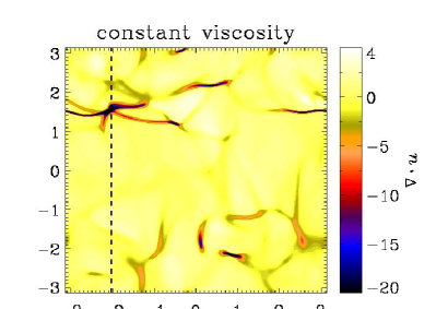
Figure 4: Grey (or color) scale representation of $\mbox{\boldmath$\nabla$}{}\cdot{\bm{u}}$ (left) and $B_{z}$ (right) in an $xy$ cross-section through $z=0$ for $\mbox{\rm Ma}=1.1$ using constant viscosity (Run 3a of Haugen et al. 2004b with $512^{3}$ meshpoints). [Adapted from Haugen et al. (2004b).]

2.2 Do shocks kill dynamos?

In the interstellar medium the flows are generally supersonic and in places even highly supersonic. Naively, one could think of highly supersonic turbulence as being nearly irrotational, in which case the dynamo should actually become much more efficient and the growth rate should increase with Mach number (Kazantsev et al. 1985). This is now known not to be the case: in a mixture of irrotational ($\mbox{\boldmath$\omega$}{}\equiv\mbox{\boldmath$\nabla$}{}\times{\bm{u}}=0$) and solenoidal ($\mbox{\boldmath$\nabla$}{}\cdot{\bm{u}}=0$) flows the critical values of the magnetic Reynolds number for the onset of dynamo action does actually increase as a function of the ratio $\sigma\equiv\langle(\mbox{\boldmath$\nabla$}{}\cdot{\bm{u}})^{2}\rangle/\langle\mbox{\boldmath$\omega$}{}^{2}\rangle$ (Rogachevskii & Kleeorin 1997). However, the ratio $\sigma$ is found to stay finite in the limit of large Mach numbers (Porter et al. 1998, Padoan & Nordlund 1999). This explains the recent finding that minimum magnetic Reynolds number for dynamo action displays a bimodal behavior as a function of the Mach number $\mbox{Ma}=u_{\rm rms}/c_{\rm s}$ (Haugen et al. 2004b). In fact, for $\mbox{Pr}_{\rm M}=1$, they find $R_{\rm m,crit}\approx 35$ for $\mbox{Ma}\ll 1$ and $R_{\rm m,crit}\approx 80$ for $\mbox{Ma}\gg 1$. For $\mbox{Pr}_{\rm M}=5$, the critical values are a bit lower (25 and 50 respectively); see Fig. 3. Indeed, in these simulations the ratio $\sigma$ is always about 1/4. Visualizations of the magnetic field show that the effects of shocks is rather weak; see Fig. 4, where we compare both cases.

It is worth noting that the use of a shock capturing viscosity (not used in the calculations presented in Fig. 4) seems to reproduce the critical values of the magnetic Reynolds number rather well; see the left hand panel of Fig. 3. In Fig. 5 we compare kinetic and magnetic energy spectra for the constant and shock-capturing viscosity solutions. The two show excellent agreement at low wavenumbers. At high wavenumbers there are major differences. The direct simulations show an extended diffusion range which is rather from the diffusive subrange in incompressible simulations (e.g. Kaneda et al. 2003). The large extent of this diffusive subrange in supersonic turbulence is obviously the reason for the tremendously high resolution needed in the direct simulations. Fortunately, as far as dynamo action is concerned, this extended subrange does not need to be fully resolved and it suffices to just cut it off with a shock-capturing viscosity.

Figure 5: Energy spectra for Runs 1a and 1c of Haugen et al. (2004b). The dotted lines give the result using shock-capturing viscosity. [Adapted from Haugen et al. (2004b).]

3 Large scale dynamos

There are some major uncertainties in what exactly are the relevant large scale dynamo mechanisms in galaxies and stars. Simulations have enabled us to make close contact between simulations and theory. We are therefore beginning to see some significant progress in that many of the uncertainties intrinsic to mean field dynamo theory can now be eliminated. However, the anticipated agreement between theory and simulations does not yet extend to the more realistic cases with strong inhomogeneities and anisotropies, for example where the turbulence is driven by convection, supernovae, or by the magneto-rotational instability.

Crucial to improving the agreement between theory and simulations has been the realization that the dominant nonlinear feedback comes from the current helicity term. This term can produce a “magnetic $\alpha$ effect” (which is $\alpha_{\rm M}={\textstyle{1\over 3}}\tau\overline{{\bm{j}}\cdot{\bm{b}}}/\rho_{0}$ in the isotropic case) – even if there is no kinetic $\alpha$ effect. The latter is $\alpha_{\rm K}=-{\textstyle{1\over 3}}\tau\overline{\mbox{\boldmath$\omega$}{}\cdot{\bm{u}}}$ in the isotropic case, where $\mbox{\boldmath$\omega$}{}=\mbox{\boldmath$\nabla$}{}\times{\bm{u}}$ is the vorticity, ${\bm{j}}=\mbox{\boldmath$\nabla$}{}\times{\bm{b}}/\mu_{0}$ the current density, and $\rho_{0}$ the mean density. An example where $\alpha_{\rm M}$ can be generated – even with $\alpha_{\rm K}=0$ – is the shear-current effect of Rogachevskii & Kleeorin (2003, 2004).

Figure 6: Evolution of the energies of the total field $\langle{\bm{B}}^{2}\rangle$ and of the mean field $\langle\overline{\bm{B}}^{2}\rangle$, in units of $B_{\rm eq}^{2}$, for runs with non-helical forcing and open or closed boundaries; see the solid and dotted lines, respectively. The inset shows a comparison of the ratio $\langle\overline{\bm{B}}^{2}\rangle/\langle{\bm{B}}^{2}\rangle$ for nonhelical ($\alpha=0$) and helical ($\alpha>0$) runs. For the nonhelical case the run with closed boundaries is also shown (dotted line near $\langle\overline{\bm{B}}^{2}\rangle/\langle{\bm{B}}^{2}\rangle\approx 0.07$). Note that saturation of the large scale field occurs on a dynamical time scale; the resistive time scale is given on the upper abscissa.

Recently, quantitative comparisons between theory and simulations have shown that whatever mean electromotive force ($\overline{\mbox{\boldmath${\cal E}$}}{}\equiv\overline{{\bm{u}}\times{\bm{b}}}$) is produced by the mean field dynamo, this produces magnetic helicity in the large scale field. Because of magnetic helicity conservation, a corresponding negative contribution in the magnetic helicity of the small scale magnetic field must be generated. This results in the production of a small scale current helicity which enters in the mean field equations as a magnetic alpha effect. To satisfy magnetic helicity conservation at all times, the small scale magnetic helicity equation (or equivalently the evolution equation for $\alpha_{\rm M}$) has to be solved simultaneously with the mean field equations. This reproduces quantitatively the resistively slow saturation of helically forced dynamos in a periodic box (Field & Blackman 2002, Blackman & Brandenburg 2002, Subramanian 2002). The explicitly time-dependent evolution equation for the magnetic $\alpha$ effect was first derived by Kleeorin & Ruzmaikin (1982). Early work by Ruzmaikin (1981) focused attention on the possibility of chaotic dynamics introduced by this effect (see also subsequent work by Schmalz & Stix 1991 and Covas et al. 1997), and the first connection between dynamical and catastrophic quenching was made by Kleeorin et al. (1995).

In order to avoid too much repetition with recent reviews on this subject (e.g., Brandenburg et al. 2002) we discuss here only in a few words the main consequences of the dynamical quenching model. It reproduces quantitatively the resistively slow saturation phase of an $\alpha^{2}$ dynamo in a periodic box (Field & Blackman 2002). Secondly, it reproduces reasonably accurately the saturation amplitude and the cycle period of $\alpha\Omega$ dynamos with a sinusoidal shear profile in a periodic box.

In the case of galaxies the dynamical time scale is $10^{7}\,{\rm yr}$, which puts rather stringent constraints if one wants to explain microgauss field strengths in very young galaxies that are $10^{9}\,{\rm yr}$ old. It is likely that a successful dynamo has to have magnetic helicity fluxes that allow the dynamo to get rid of small scale magnetic helicity to allow for a rapid build-up of a large scale field that tends to have magnetic helicity of the opposite sign (Blackman & Field 2000, Kleeorin et al. 2000). The currently most convincing example where the presence of boundaries has been found to be important is in connection with turbulent dynamos that work mainly in the presence of shear (Brandenburg et al. 2005). Here, the main effect that is thought to be responsible is the so-called shear–current effect where the electromotive force has a component proportional to $\overline{\bm{W}}\times\overline{\bm{J}}$. Here, $\overline{\bm{W}}$ is the vorticity of the mean flow and $\overline{\bm{J}}$ is the mean current density. This effect is technically related to the $\mbox{\boldmath$\Omega$}{}\times\overline{\bm{J}}$ effect (e.g. Krause & Rädler 1980), which is obviously quite distinct from the famous $\alpha$ effect. Another possibility is the Vishniac & Cho (2001) mechanism. However, it has not yet been possible to verify any of them explicitly. Preliminary mean field calculations suggest, however, that the $\overline{\bm{W}}\times\overline{\bm{J}}$ effect produces qualitatively favorable agreement with the direct simulations.

Figure 6 shows that in the presence of closed (i.e. perfectly conducting) boundaries, magnetic energy both of the total field and of the mean field saturates at a much lower level than with open boundaries ($\mbox{\boldmath$n$}{}\times{\bm{B}}=0$). The inset shows the ratio between the energies contained in the mean field to that in the total field. Note that this ratio stays small when the boundaries are closed, but it increases to fairly large values (around 0.7) when the boundaries are open.

4 Conclusions

In many astrophysical bodies some type of large scale dynamo is likely to operate. This dynamo may operate with nonhelical turbulence and shear alone, i.e. without $\alpha$ effect. Small scale dynamos, on the other hand, are an extreme case which requires that there is no shear and no helicity, for example. Both types of dynamos are vulnerable in their own ways: a large scale dynamo requires magnetic and current helicity fluxes in order to be successful, while small scale dynamos may require magnetic Prandtl numbers that are not too small. However, as we have shown in the present paper, small scale dynamos still work in the compressible regime. In fact, it now seems that, once the Mach number exceeds unity, its onset becomes independent of the Mach number. This hypothesis has only been tested for small Mach numbers, so it would be useful to extent these studies to larger values. However, as we have also been able to show, the use of shock-capturing viscosities seems to be a reasonably accurate approximation for this purpose.

References

- [] Batchelor, G. K. 1959, JFM, 5, 113
- [] Beck, R., Brandenburg, A., Moss, D., Shukurov, A., & Sokoloff, D. 1996, ARA&A, 34, 155
- [] Boldyrev, S., & Cattaneo, F. 2004, PRL, 92, 144501
- [] Blackman, E. G., & Field, G. F. 2000, MNRAS, 318, 724
- [] Blackman, E. G., & Brandenburg, A. 2002, ApJ, 579, 359
- [] Brandenburg, A. 2001, ApJ, 550, 824
- [] Brandenburg, A., Dobler, W., & Subramanian, K. 2002, AN, 323, 99
- [] Brandenburg, A., Haugen, N. E. L., Käpylä, P. J., & Sandin, C. 2005, AN, astro-ph/0412364
- [] Cho, J., Lazarian, A., & Vishniac, E. 2002, ApJ, 566, L49
- [] Covas, E., Tworkowski, A., Brandenburg, A., & Tavakol, R. 1997, A&A, 317, 610
- [] Dobler, W., Haugen, N. E. L., Yousef, T. A., & Brandenburg, A. 2003, PRE, 68, 026304
- [] Field, G. B., & Blackman, E. G. 2002, ApJ, 572, 685
- [] Haugen, N. E. L., Brandenburg, A., & Dobler, W. 2003, ApJ, 597, L141
- [] Haugen, N. E. L., Brandenburg, A., & Dobler, W. 2004a, PRE, 70, 016308
- [] Haugen, N. E. L., Brandenburg, A., & Mee, A. J. 2004b, MNRAS, 353, 947
- [] Kaneda, Y., Ishihara, T. Yokokawa, M., Itakura, K., & Uno, A. 2003, Phys. Fluids, 15, L21
- [] Kazantsev, A. P. 1968, Sov. Phys. JETP, 26, 1031
- [] Kazantsev, A. P., Ruzmaikin, A. A., & Sokoloff, D. D. 1985, Sov. Phys. JETP, 88, 487
- [] Kleeorin, N. I., & Ruzmaikin, A. A. 1982, Magnetohydrodynamics, 18, 116
- [] Kleeorin, N. I, Rogachevskii, I., & Ruzmaikin, A. 1995, A&A, 297, 159
- [] Kleeorin, N. I, Moss, D., Rogachevskii, I., & Sokoloff, D. 2000, A&A, 361, L5
- [] Krause, F., & Rädler, K.-H. 1980, Mean-Field Magnetohydrodynamics and Dynamo Theory (Akademie-Verlag, Berlin; also Pergamon Press, Oxford)
- [] Moffatt, H. K. 1963, JFM, 17, 225
- [] Padoan, P., & Nordlund, Å. 1999, ApJ, 526, 279
- [] Porter, D. H., Woodward, P. R., & Pouquet, A. 1998, Phys. Fluids, 10, 237
- [] Rogachevskii, I. & Kleeorin, N. 1997, PRE, 56, 417
- [] Rogachevskii, I., & Kleeorin, N. 2003, PRE, 68, 036301
- [] Rogachevskii, I., & Kleeorin, N. 2004, PRE, 70, 046310
- [] Ruzmaikin, A. A. 1981, Comments Astrophys., 9, 85
- [] Schekochihin, A. A., Cowley, S. C., Maron, J. L., McWilliams, J. C. 2004, PRL, 92, 054502
- [] Schmalz, S., & Stix, M. 1991, A&A, 245, 654
- [] Subramanian, K. 2002, Bull. Astr. Soc. India, 30, 715
- [] Vishniac, E. T., & Cho, J. 2001, ApJ, 550, 752