Regimes of Stability and Scaling Relations for the Removal Time in the Asteroid Belt: A Simple Kinetic Model and Numerical Tests

Abstract

We report on our theoretical and numerical results concerning the transport mechanisms in the asteroid belt. We first derive a simple kinetic model of chaotic diffusion and show how it gives rise to some simple correlations (but not laws) between the removal time (the time for an asteroid to experience a qualitative change of dynamical behavior and enter a wide chaotic zone) and the Lyapunov time. The correlations are shown to arise in two different regimes, characterized by exponential and power-law scalings. We also show how is the so-called ”stable chaos” (exponential regime) related to anomalous diffusion. Finally, we check our results numerically and discuss their possible applications in analyzing the motion of particular asteroids.

1 Introduction

Despite some important breakthroughs in research of transport mechanisms in the Solar system in the past decade, we still lack a general quantitative theory of chaotic transport, which is especially notable for the so-called stable chaotic bodies. In this paper, we sketch a new kinetic approach, which, in our opinion, has a perspective of providing us such a theory sometime in the future.

A kinetic model of transport has already been proposed by [Murray & Holman (1997)]. Although it is an important step forward, this model fails to include a number of important effects. We also wish to emphasize the role of phase space topology in the transport processes. This has only recently been understood in papers by [Tsiganis, Varvoglis & Hadjidemetriou (2000), Tsiganis, Varvoglis & Hadjidemetriou (2002a), Tsiganis, Varvoglis & Hadjidemetriou (2002b), Tsiganis, Varvoglis & Hadjidemetriou (2000, 2002a, 2002b)]. Still, the exact role of cantori and stability islands in various resonances remains unclear. This is one of the issues we intend to explore in this paper. We argue that, due to the inhomogenous nature of the phase space, a separate kinetic equation for each transport mechanism should be constructed; after that, one can combine them to obtain the description of long-time evolution. This is the basic idea of our approach, which leads to some interesting statistical consequences, such as anomalous diffusion and approximate scaling of removal times with Lyapunov times.

2 The kinetic scheme

In order to model the transport, we use the ”building block approach” we have recently developed for Hamiltonian kinetics ([Čubrović (2004), Čubrović 2004]). We use the Fractional Kinetic Equation (FKE), a natural generalization of the diffusion equation for self-similar and strongly inhomogenous media ([Zaslavsky (2002), e. g. Zaslavsky 2002]):

$$\frac{\partial^{\beta}f\left(I,t\right)}{\partial t^{\beta}}=\frac{\partial^{\alpha}}{\partial|I|^{\alpha}}\left[\mathcal{D}\left(I\right)f\left(I,t\right)\right]$$ (1)

Thus, the evolution of the distribution function $f(I,t)$ is governed by the transport coefficient $\mathcal{D}$ (the generalization of the diffusion coefficient) and by the (non-integer, in general) order of the derivatives $\alpha$ ($0<\alpha\leq 2$) and $\beta$ ($0<\beta\leq 1$). The quantity $\mu\equiv 2\beta/\alpha$ is called the transport exponent (for the second moment the following holds asymptotically: $\langle\Delta I^{2}\rangle\propto t^{\mu}$). If $\mu\neq 1$, the transport is called anomalous (in contrast to normal transport or normal diffusion).

We shall now very briefly describe each of the four building blocks; unfortunately, most equations are cumbersome and complicated, so we limit ourselves in this paper (for the sake of conciseness) to merely state the basic ideas and final results of the method. We use the planar MMR Hamiltonians $H_{2BR}=H_{2BR}^{0}+H_{2BR}^{\prime}$ and $H_{3BR}=H_{3BR}^{0}+H_{3BR}^{\prime}$ for two- and three-body resonances, taken from [Murray, Holman & Potter (1998)] and [Nesvorny & Morbidelli (1999)], respectively. Under $H^{0}$ we assume the action-only part of the Hamiltonian. $H_{2BR}$ was modified to account for the purely secular terms; also, both Hamiltonians were modified to include the proper precessions of Jupiter and Saturn:

$$H_{2BR}^{\prime}=\sum_{m=0,1;s=0\ldots k_{J}-k}^{u_{5},u_{6}}c_{msu_{5}u_{6}}\cos\left[m\left(k_{J}\lambda_{J}-k\lambda\right)+sp+\left(u_{5}g_{5}+u_{6}g_{6}\right)t+u_{5}\beta_{J}+u_{6}\beta_{S}\right]$$ (2)

$$H_{3BR}^{\prime}=\sum_{m=0,1;s}^{u_{5},u_{6}}c_{msu_{5}u_{6}}\cos\left[m\left(k_{J}\lambda_{J}+k_{S}\lambda_{S}+k\lambda\right)+sp+\left(u_{5}g_{5}+u_{6}g_{6}\right)t+u_{5}\beta_{J}+u_{6}\beta_{S}\right]$$ (3)

The notation is usual. In $H_{2BR}^{\prime}$, we include all the existing harmonics; in $H_{3BR}^{\prime}$, we include only those given in [Nesvorny & Morbidelli (1999)]. In what follows, we shall consider only the diffusion in eccentricity, i. e. $P$ Delauney variable. Inclusion of the inclination could be important but we postpone it for further work.

We estimate the transport coefficient as:

$$\mathcal{D}=\frac{T_{lib}^{(\alpha-\beta)}}{2}\sum_{s}s^{\alpha}P^{s\alpha}\left(\sum_{u_{5},u_{6}}c^{\prime}_{0su_{5}u_{6}}(\alpha)+jc^{\prime}_{1su_{5}u_{6}}(\alpha)\right)$$ (4)

where $T_{lib}$ denotes the libration period while $c_{msu_{5}u_{6}}^{\prime}$ are coefficients dependent on the exponent $\alpha$ from (1), independent on angles and $P$, which were computed using the algorithm from [Ellis & Murray (2000)], for $H_{2BR}$, or taken from [Nesvorny & Morbidelli (1999)], for $H_{3BR}$. The indicator $j$ can be equal to $0$ or $1$ (i. e. omission or inclusion of the resonant terms), depending on the building block (see bellow). Although we were able to compute also the higher-order corrections to this quasilinear result in some cases, we neglect them in what follows, in order to be able to solve the FKE analytically.

The first class of building blocks we consider are the overlapping stochastic layers of subresonances. In this case, one expects a free, quasi-random walk continuous in both time and space, since no regular structures are preserved. Therefore, the FKE simplifies to the usual diffusion equation, i. e. we have $\alpha=2$, $\beta=1$ in (4); also, $j=1$ (the resonant harmonics are actually the most important ones).

The above reasoning is only valid if the overlapping of subresonances is not much smaller than $1$. Otherwise, the diffusion can only be forced by the secular terms. Also, long intervals between subsequent ”jumps” induce the so-called ”erratic time”, i. e. $\beta$ can be less than $1$, its value being determined by the distribution of time intervals between ”jumps” $p(\Delta t)=1/\Delta t^{1+\beta}$. So, the transport coefficient (4) now has $j=0$, $\alpha=2$ and $\beta<1$.

Our third class of building blocks are the resonant stability islands. To estimate $\beta$ we use the same idea as in the previous case; after that, we compute $\alpha$ from $\beta$ and $\mu$, the transport exponent, which we deduce using the method developed in [Afraimovich & Zaslavsky (1997)]. Namely, analytical and numerical studies strongly suggest a self-similar structure characterized by a power-law scaling of trapping times $\lambda_{T}$, island surfaces $\lambda_{S}$ and number of islands $\lambda_{N}$ at each level. The transport exponent is then equal to $\lambda_{N}\lambda_{S}/\lambda_{T}$. For some resonances and for some island chains, we computed the scaling exponents applying the renormalization of the resonant Hamiltonian as explained in [Zaslavsky (2002)]; in the cases when we did not know how to do this, we used the relation between the transport exponent and the fractal dimension $d_{T}$ of the trajectory in the $(P,p)$ space (the space spanned by the action $P$ and the conjugate angle $p$), which is actually the dimension of the Poincare section of the trajectory:

$$d_{T}=\frac{2\lambda_{T}}{\lambda_{N}\lambda_{S}}$$ (5)

The last remaining class of blocks are cantori. Here, we assume the scaling of gap area on subsequent levels with exponent $\lambda_{S}$ and an analogous scaling in trapping probability with exponent $\lambda_{p}$, which determines the transport exponent as $2\ln\lambda_{p}/\ln\lambda_{S}$; see also the reasoning from [Shevchenko (1998)]. The scaling exponents were estimated analogously to the previous case.

For each building block, we construct a kinetic equation and solve it. We always put a reflecting barrier at zero eccentricity and an absorbing barrier at the Jupiter-crossing eccentricity. The solution in Fourier space $(q,t)$ can be written approximately in the following general form:

$$f_{i}(q,t)=E_{\beta}(-|q^{\alpha}|\star\hat{\mathcal{D}_{i}}t^{\beta})$$ (6)

where $E_{\beta}$ stands for the Mittag-Leffler function and $\hat{\mathcal{D}_{i}}$ denotes the Fourier transform of $\mathcal{D}_{i}$. The index $i$ denotes a particular building block. The key for obtaining the global picture is to perform a convolution of the solutions for all the building blocks. Furthermore, one must take into account that the object can start in different blocks and also that, sometimes, different ordering of the visited blocks is possible. Therefore, one has the following sum over all possible variations of blocks (we call it Equation of Global Evolution - EGE):

$$f(P,t)=\sum\left[p_{1}f_{1}(P,t)\star p_{2}f_{2}(P,t)\star\dots\star p_{i}f_{i}(P,t)\star\dots\right]$$ (7)

To calculate it, one has to know also the transition probabilities $p_{i}$, which is not possible to achieve solely by the means of analytic computations. That is why we turn again to semi-analytic results.

3 Removal times, Lyapunov times and $T_{L}$ – $T_{R}$ correlations

The first task is to determine the relevant building blocks and transitional probabilities. We do that by considering the overviews of various resonances as given in [Moons & Morbidelli (1995), Morbidelli & Moons (1993), Moons, Morbidelli & Migliorini (1998)]. For the resonances not included in these references, we turn again to the inspection of Poincare surfaces of section, integrating the resonant models (2) and (3). In this case, the probabilities are estimated as the relative measures of the corresponding trajectories on the surface of section.

The result of solving the EGE is again a Mittag-Leffler function:

$$f_{global}(q,t)=E_{\gamma}(-|q|^{\delta}t^{\gamma})$$ (8)

The asymptotic behavior of this function, described e. g. in [Zaslavsky (2002)], has two different forms: the exponential one and the power-law one, depending on the coefficients $\gamma$ and $\delta$, which are determined by the probabilities $p_{i}$ and transport coefficients and exponents of the building blocks. In the small $\gamma$ limit, the behavior is exponential and the second momentum scales with $\tau_{cross}$, where $\tau_{cross}$ is the timescale of crossing a single subresonance, which we interpret as the Lyapunov time. When $\gamma$ becomes large and the role of stickiness more or less negligible, one gets a power-law dependance on $\tau_{cross}$, i. e. $T_{L}$. So, we have the expressions:

$$T_{R}\propto\exp\left(T_{L}^{x}\right)\Phi\left(\Lambda_{0},\cos(\ln P_{0}),Q_{0}\right)$$ (9)

for the exponential or stable chaotic regime, and:

$$T_{R}\propto\left(T_{L}^{y}\right)\Phi\left(\Lambda_{0},\cos(\ln P_{0}),Q_{0}\right)$$ (10)

for the power-law regime. The scalings are not exact because the fluctuational terms $\Phi\left(\Lambda_{0},P_{0},Q_{0}\right)$ appear. These terms are log-periodic in $P_{0}$ and can explain the log-normal tails of the $T_{R}$ distribution, detected numerically e. g. in [Tsiganis, Varvoglis & Hadjidemetriou (2000)].

4 Results for particular resonances

We plan to do a systematic kinetic survey of all the relevant resonances in the asteroid belt. Up to now, we have only preliminary results for some resonances.

Table 1 sums up our results for all the resonances we have explored. For each resonance, we give our analytically calculated estimates for $T_{L}$ and $T_{R}$. We always give a range of values, obtained for various initial conditions inside the resonance. If the ”mixing” of the phase space is very prominent, we sometimes get a very wide range, which includes both normal and stable chaotic orbits. One should note that the ”errorbars” in the plot are simply the intervals of computed values – they do not represent the numerical errors. We also indicate if the resonance has a resonant periodic orbit, which is, according to [Tsiganis, Varvoglis & Hadjidemetriou (2002b)], the key property for producing the fast chaos. Bulirsch-Stoer integrator with Jupiter and Saturn as perturbers was used for the integrations.

We have also tried to deduce the age of the Veritas family, whose most chaotic part lies inside the $5-2-2$ resonance. Our EGE gives an approximate age about 9 Myr while, assuming a constant diffusion coefficient (Knežević, personal communication), one gets about 8.3 Myr. The similarity is probably due to the young age of the family: were it older, the effects of non-linearity would prevail and our model would give an age estimate which is substantially different from that obtained in a linear approximation.

Table 1: Analytical and numerical values of the Lyapunov time (in Kyr) and removal time (in Myr). Existence of the periodic orbit in the planar problem for the 2BR is also indicated; the data in this column were taken from [Tsiganis, Varvoglis & Hadjidemetriou (2002b)].

Resonance	$T_{L}$ (Kyr)	$T_{L}^{Num}$ (Kyr)	$T_{R}$ (Myr)	$T_{R}^{Num}(Myr)$	Per. orbit ?
$2:1$	1.1–3.4	2.9–5.2	0.8–19.4	1.1–31.2	Yes
$3:2$	1.4–3.5	3.1–6.2	0.9–19.1	3.2–142.7	Yes
$3:1$	6.2–8.2	6.8–9.4	0.8–8.0	1.0–21.2	Yes
$5:3$	1.9–2.2	1.1–3.5	0.9–4.1	0.8–7.4	Yes
$5:2$	6.9–9.2	8.3–14.4	7.6–13.4	9.2–28.7	Yes
$7:4$	2.7–5.3	1.8–3.9	6.9–23.4	12.2–41.3	Yes
$8:5$	3.7–6.7	4.1–7.6	8.2–18.2	7.3–23.4	No
$7:3$	5.0–6.9	6.9–9.1	16.7–62.2	22.4–91.2	No
$9:5$	5.4–6.8	3.1–5.2	23.2–86.7	11.3–104.2	No
$11:7$	7.1–14.1	3.4–9.7	10.6–73.4	8.4–88.2	Yes
$11:6$	10.8–22.7	10.1–16.5	16.4–330.3	13.2–$\approx 500$	No
$12:7$	11.1–14.7	4.1–15.2	4.6–278.1	5.2–$\approx 1000$	No
$13:7$	65.1–84.6	43.3–76.1	23.2– $\approx 1000$	14.2– $>1000$	No
$13:6$	55.1–77.6	14.6–24.5	41.3– $\approx 1000$	21.1– $>1000$	No
$18:7$	$\approx 500$	300-600	$\approx 20000$	$>1000$	No
$5-2-2$	11.4–13.7	8.4—10.9	$\approx 10000$	$>1000$	No
$2+2-1$	90–160	130–240	$\approx 20000$	$>1000$	No
$6+1-3$	130–150	130–170	$\approx 40000$	$>1000$	No

Figure 1 gives the results from table 1 plotted along the semimajor axis. It can be noted that the agreement is good within an order of magnitude, with some exceptions. Actually, one can see that the disagreement with the simulations is most significant exactly in the resonances with a periodic orbit, which might actually require a completely different treatment of transport.

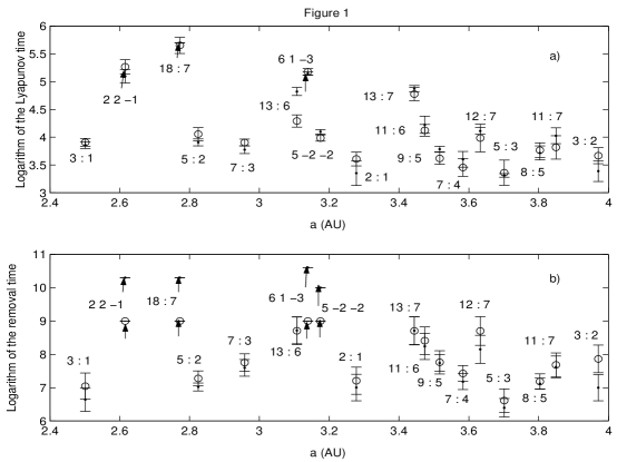
Figure 1: Analytical (points) and numerical (circles) values from table 1, for Lyapunov time (a) and removal time (b). Arrows correspond to extremely uncertain numerical values, usually the values close to or larger than the integration timespan (1 Gyr).

In figure 2, we plot the numerical $T_{L}$ – $T_{R}$ relation for the resonances $5:3$ and $12:7$, examples of normal and stable chaos, respectively. The largest discrepancies in the figure 2a are probably for the objects near the stability islands; in the figure 2b, the fit is completely ruined. To cheque the assumption that this is due to the mixing of populations, we integrate a larger population of objects and divide them into two classes (the criterion being the prominence of anomalous diffusion, see later). For each class, we perform a separate fit with the corresponding $T_{L}$ – $T_{R}$ relation. Now most objects can be classified into one of the two scaling classes. In particular, this shows that the famous stable-chaotic object 522 Helga is probably not a remnant of some larger initial population but rather a member of one of the two populations existing in this resonance.

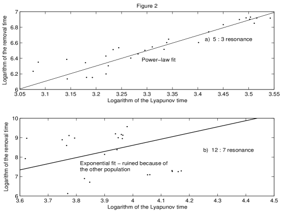
Figure 2: Plot of $T_{L}$ – $T_{R}$ dependance for the resonances $5:3$ (a), fit with a power-law, and $12:7$ (b), fit with the exponential law. The exponential fit also looks linear, due to obviously bad fit quality. See text for comments.

Figure 3: The same as in figure 2b but with two separate plots for the exponential regime population, and for the power-law regime population. Obviously, we have a substantially better fit.

Finally, in figure 4, we give the time evolution of the dispersion in $P$ (i. e. $\langle\Delta P^{2}\rangle$) for a set of clones of 522 Helga, using the procedure described in [Tsiganis, Anastasiadis & Varvoglis (2000)]. Anomalous diffusion is clearly visible. This confirms the stable chaotic nature of this object and shows that we can use the anomalous character of diffusion as an indicator of stable chaos.

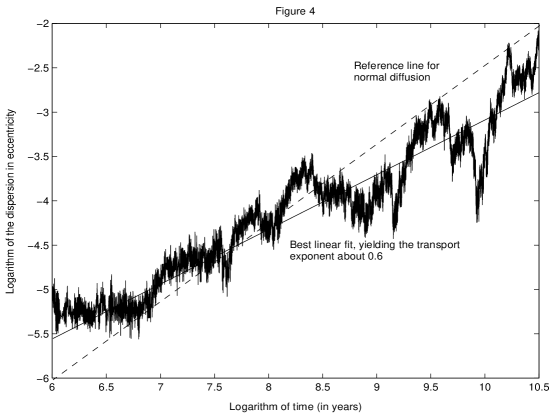
Figure 4: Diffusion in eccentricity for a set of clones of 522 Helga. Domination of anomalous transport is obvious. The reference line for normal diffusion ($\mu=1$) is also plotted.

5 Conclusions and discussion

We have given a kinetic model of chaotic transport in the asteroid belt, based on the concept of convolution of various building blocks. Combining numerical and analytical results, we have shown how the removal time can be calculated and interrelated with the Lyapunov time. We have obtained two regimes for chaotic bodies, the power-law one and the exponential one. Due to the fractal structure of the phase space, however, asteroids from different regimes can be ”mixed” in a small region of the phase space.

We would like to comment briefly on the controversial issue of the $T_{L}$ – $T_{R}$ relation. First of all, the correlations we have found are of statistical nature only and should not be regarded as ”laws” in the sense of [Murison, Lecar & Franklin (1994)]. Furthermore, due to their statistical nature, they cannot be used for any particular object, only for populations. Finally, it is clear that the scalings are non-universal, i. e. the scaling exponents are different for different resonances (possibly also in disconnected regions of a single resonance).

The exponential regime, characterized mainly by anomalous transport through various quasi-stable structures, corresponds to the stable chaotic regime, discussed e. g. in [Tsiganis, Varvoglis & Hadjidemetriou (2000)] and [Tsiganis, Varvoglis & Hadjidemetriou (2002a)]. The reason that the exponential $T_{L}$ – $T_{R}$ correlation was not noticed thus far are in part very large values of $T_{R}$ in this regime, and in part the fact that stable chaotic objects are typically mixed with the objects in the normal chaotic regime. Also, it is interesting to note that the exponential scalings are of the same form as those predicted in [Morbidelli & Froeschlé (1996)] for the Nekhoroshev regime; therefore, it seems that the exponential stability can arise also due to stickyness, not necessarily as a consequence of the Nekhoroshev structure.

Finally, we hope that our research will stimulate further work in this field, since the results presented here are no more than just a sketch of possible general theory.