Adaptive Scheduling Algorithms for Planet Searches

Abstract

High-precision radial velocity planet searches have surveyed over $\sim\!2000$ nearby stars and detected over $\sim\!200$ planets. While these same stars likely harbor many additional planets, they will become increasingly challenging to detect, as they tend to have relatively small masses and/or relatively long orbital periods. Therefore, observers are increasing the precision of their observations, continuing to monitor stars over decade timescales, and also preparing to survey thousands more stars. Given the considerable amounts of telescope time required for such observing programs, it is important use the available resources as efficiently as possible. Previous studies have found that a wide range of predetermined scheduling algorithms result in planet searches with similar sensitivities. We have developed adaptive scheduling algorithms which have a solid basis in Bayesian inference and information theory and also are computationally feasible for modern planet searches. We have performed Monte Carlo simulations of plausible planet searches to test the power of adaptive scheduling algorithms. Our simulations demonstrate that planet searches performed with adaptive scheduling algorithms can simultaneously detect more planets, detect less massive planets, and measure orbital parameters more accurately than comparable surveys using a non-adaptive scheduling algorithm. We expect that these techniques will be particularly valuable for the N2K radial velocity planet search for short-period planets as well as future astrometric planet searches with the Space Interferometry Mission which aim to detect terrestrial mass planets.

1. Introduction

Radial velocity planet searches have surveyed over 2000 nearby solar type stars and discovered over 200 planets. The surveys require many high precision radial velocity observations of each star in the survey, and hence a significant amount of observing time. For example, the N2K project has recently begun surveying the next $\sim 2000$ nearby stars for planets. This project aims to discover dozens of hot Jupiters and hopefully additional transiting planets (Fischer et al. 2004). Given the large target list for the N2K project, it is essential that inferences about the presence of planets and their orbits be made as efficiently as possible. The observing program aims to take three observations of each star on consecutive nights, followed by an additional observation one to a few months later. In many cases, it is clear after a few observations that the radial velocity observations have a dispersion significantly greater than would be expected due to measurement errors only. However, there may still be a large range of possible orbital solutions, and several additional observations will often be required to determine the planetary orbits. Given the considerable observation time required for such planet searches and the value of telescope time, it is important that these surveys be as efficient as possible.

Previous studies have demonstrated that a variety of observing schedules result in comparable efficiencies for detecting planets (Sozzetti 2002, Ford 2004). However, these studies have only considered non-adaptive observing schedules, i.e., schedules that are fully determined before any observations are taken. In this paper, we develop and test the efficiency of adaptive scheduling algorithms. We describe how adaptive scheduling algorithms can help increase the efficiency of planet searches by utilizing the information available from the previous observations to plan future observations.

Adaptive scheduling algorithms can be based on Bayesian inference (Loredo 2004). Within this framework, the need to make decisions is minimized. For example, the experimenter does not say that a planet has been detected, but rather states that the posterior probability for the null hypothesis is some small value. This eliminates the need to chose threshold functions. More importantly, by eliminating decisions and basing the scheduling algorithm on the posterior probability distribution, the posterior probability distribution is not biased by the choice of observing schedule. Additionally, it is straightforward to test new hypotheses which will inevitably be formulated after making some observations. For these reasons, we have developed adaptive scheduling algorithms within the Bayesian framework, always considering all possible models (weighted according to their posterior probability).

It should be noted that the use of adaptive scheduling algorithms — even those based on Bayesian inference— does affect the distribution of the posterior distributions. Indeed, that is the purpose of employing such algorithms. For example, if an adaptive scheduling algorithm is chosen to increase the sensitivity of an observing program for detecting planets, then it is expected that an ensemble of surveys employing the adaptive scheduling algorithm will result in detecting more planets than a comparable ensemble of surveys using a fixed scheduling algorithm. It should be noted that this is also true of non-adaptive scheduling algorithms. For example, an observing program which makes observations over a long duration will be sensitive to planets with orbital periods comparable or less than the survey duration, but there may be ambiguities in determining the orbital period associated with aliasing. If an observing program obtained the same number of observations with the same precision, but performed all the observations during a smaller interval of time, then the shorter survey would be less sensitive to planets with orbital periods longer that the short survey’s duration, but would likely reduce aliasing ambiguities for short period planets. Thus, when analyzing the properties of a population of stars and planets, it is alway important to account for the scheduling algorithm used.

Our approach applies the principles of Bayesian inference and information theory to guide the choice of observation times (and later choice of target stars). Following Loredo (2004), we assume a prior for both the probability that each target star has a planet and the distribution of orbital periods and masses of planets. Second, a small number of observations are taken of each target star. Bayesian inference is used to calculate the posterior probability distribution for all model parameters. Then, the posterior probability distribution for the model parameters is used to calculate the predictive distribution, the posterior probability distribution for the radial velocities at some future time. By comparing the information contained in the predictive distribution at various future times, it is possible to choose observing times at which additional observations would be most valuable. This technique requires performing integration over several variables and in general is extremely computationally intensive. In this paper we describe a relatively fast algorithm for performing the necessary integrations.

While it would be desirable to observe each star in a survey at the optimal times for each particular star, it is more realistic to consider a planet survey which is able to perform a fixed number of observations at specific times. In this case, the information contained in the predictive distributions for several stars can be used to select which target star should be observed at a given time.

We describe the algorithm for choosing observing times of a single star in §2. In §3 we describe a generalized algorithm that allows for multiple target stars, along with simulations which demonstrate the power of adaptive scheduling algorithms. In §4 we present generalizations that allow observing schedules to be optimized for meeting specific goals, such as detecting planets in the habitable zone or maximizing the number of planets detected. Finally, we discuss the implications of our findings and the challenges which remain in §5.

2. Adaptive Scheduling for a Single Target Star

2.1. Priors

For each target star we assume a prior probability, $p(0)$, for the null hypothesis that the radial velocity observations are consistent with a constant radial velocity. We assume a probability, $p(1)=1-p(0)$, that the star has a single planet. For the orbital parameters of any planet, we take prior distributions that are flat in $\log P$, $\log K$, and $\phi_{o}$, where $P$ is the orbital period, $K$ is the velocity semi-amplitude, and $\phi_{o}$ is the phase at a given epoch. These choices are standard for variables which represent magnitudes and angles. We limit the range of orbital parameters to $P_{\min}\leq P<P_{\max}$, $K_{\min}\leq K<\infty$, and $0\leq\phi_{o}<2\pi$ (see §2.3). The choices for the prior distributions are supported by scaling arguments as well as their approximate agreement with the orbital parameters for the known extrasolar planets.

There are a few differences in our prior distributions and the distributions of orbital elements of known extrasolar planets. First, we apply a sharp cutoff for orbital periods less than $P_{\min}$. The OGLE transit searches have discovered planets with orbital periods as short as $1.2$d (Koanacki 2003). While radial velocity searches are very sensitive to such planets, the shortest orbital period discovered by a radial velocity survey is 2.5d (Udry et al. 2003). It is important to recognize the OGLE transit search surveys a much larger number of stars than radial velocity surveys (Gaudi, Seager, & Mallen-Ornelas 2004). Thus, the observations imply that the distribution of orbital periods is roughly flat in $\log P$ for $P\geq 3d$, but there is a very significant reduction in the number of planets at shorter orbital periods (Gaudi, Seager, & Mallen-Ornelas 2004). Therefore, it would be reasonable to apply cutoff for orbital periods $P<P_{\min}$ for any $P_{\min}<3$d, and we choose $P_{\min}=2.5$d. Given recent discoveries, we do not suggest such a large $P_{\min}$ for future studies.

We also apply a sharp cutoff for orbital periods greater than $P_{\max}$. When a planet has an orbital period much longer than $T_{\mathrm{o}bs}$, then there are degeneracies in the Keplerian orbital parameters and the radial velocities can be well modeled by a quadratic polynomial (Cumming 2004). By replacing all the Keplerian models with $P\geq\pi T_{\mathrm{o}bs}$ with a single quadratic model, it is possible for our algorithm to detect planets with orbital periods, $\pi T_{\mathrm{o}bs}\leq P$ efficiently. We maintain the flat prior in $\log P$ by setting the prior probability for the quadratic model equal to the sum of the prior probabilities for orbital periods in the range $\pi T_{\mathrm{o}bs}<P<P_{\max}$. Since the prior distribution is flat in $\log P$, this relative prior probability is not sensitive to the exact choice of $P_{\max}$. The effect of varying $P_{\max}$ is to change the prior probability for a planet having a long-period orbit relative to the prior probability for a planet having an orbital period between $P_{\min}$ to $P_{\max}$. Since little is known about the abundance of extrasolar planets with orbital periods greater than $\sim 10$yr, we choose $P_{\max}=40$yr guided by our own solar system.

Another difference between our prior distributions and the distributions of orbital elements for known extrasolar planets is that we assume the planetary orbits are circular, i.e., the orbital eccentricity, $e$, is zero. Since a circular orbit approximates a Keplerian orbit with a small eccentricity, our algorithm is expected to identify planets with small and even moderately eccentric orbits. However, the efficiency for detecting planets on moderately eccentric orbits may be somewhat reduced compared to the efficiency for detecting a planet on a circular orbit with comparable mass and orbital period. The reduction in efficiency is relatively mild for $e<0.4$, but rapidly becomes more significant (Endl. et al. 2002; Cumming 2004). While many of the known extrasolar planets are on significantly eccentric orbits, the planets with shorter orbital periods tend to have smaller eccentricities. This is likely due in part to tidal circularization affecting planets with small orbital periods (Rasio, Livio, & Tout 1996). While the assumption of circular orbits is likely appropriate for many planets (especially short-period planets targeted by the N2K project), there is no question that it would be more desirable to include eccentricities. Still, the assumption of circular orbits permits significant computational advantages making it extremely attractive when a large range of parameter space must be searched (e.g., for planetary orbits which are poorly constrained by the currently available data). The reduction in computational requirements makes it computationally feasible to explore the properties of adaptive scheduling algorithms (as in this paper).

2.2. Initial Observations

Before making observations of a target star, there is no basis for believing that the star is more or less likely to have a planet or that various orbital parameters are preferred, except what is suggested by the prior probability distribution. Therefore, an initial set of $N_{\min}$ observations is made for each star. When the number of observations, $N_{\mathrm{o}bs}$ is less than $N_{\min}$, the choices for when to observe are not affected by previous observations, however these choices may be affected by practical considerations. For example, observations must be made at night and radial velocity surveys are typically allocated observing time near full Moon. Additionally, the airmass and atmospheric conditions in the direction of each target may favor observing certain targets at certain times during the available observing nights.

Under the null hypothesis, there is a single fit parameter for the constant velocity of the star, $C_{0}$, and the star’s velocity is given by $v_{*,C_{0}}(t)=C_{0}$. Next, we consider the alternative hypothesis that the star has a single planet in a circular orbit. There are four parameters which can be varied to fit the velocity observations of each star, $P$, $K$, $\phi_{o}$, and $C_{1}$, where $C_{1}$ is the constant velocity of the star. (Given the way the star’s velocity is measured, it is typically necessary to use different values of $C_{1}$ for different observatories. Thus, when there are only a small number of observations of a given target star, it is extremely advantageous if all the observations are made from a single observatory. For the purposes of this paper, we assume that all radial velocity observations are made with a single observatory.) The radial velocity signature of a planet on a circular orbit can be written as

$$v_{*,\vec{x}}(t)=K\cos\left[\frac{2\pi}{P}t+\phi_{o}\right]+C_{1}.$$ (1)

After a set of $N_{\min}=3$ initial observations, it is possible to evaluate the plausibility of the fit parameters, $P$, $K$, $\phi_{o}$, and $C_{1}$. Since each observation has some observational uncertainties, the orbit still is not uniquely determined, even if our general model is exactly correct.

As noted in §2.1, when a planet has an orbital period much longer than the time span of observations, then the fit parameters used above are not well determined by the radial velocity observations. Therefore, for orbital periods $\pi T_{\mathrm{o}bs}\leq P\leq P_{\max}$, we model the radial velocity of the star as

$$v_{*,\vec{a}}(t)=a_{0}+a_{1}t+a_{2}t^{2},$$ (2)

where $\vec{a}=\left(a_{0},a_{1},a_{2}\right)$ is the set of coefficients for the polynomial model.

2.3. Inference

Once $N_{\mathrm{o}bs}\geq N_{\min}$, we analyze the available observations using the methods of Bayesian statistics after making each new observation. The results of the analysis can be used to make informed choices for when stars should be targeted for additional observations. Let $\vec{d}$ denote the set of available data, in this case the previous radial velocity observations. We have already introduced the prior probabilities for the null hypothesis, $p(0)$, and for the single planet model, $p(1)$, as well as the prior probability distribution for orbital parameters, $p(\vec{x}|1)$. Next, we introduce the conditional probability for the observations given the null hypothesis, $p(\vec{d}|0)$, and the conditional probability for the observations given a fixed set of model parameters, $p(\vec{d}|\vec{x})$. Since the observational errors are assumed to be independent, both conditional probabilities can be simply evaluated as the product of the probabilities for drawing each observation given the relevant model for the stellar velocity. Since each radial velocity measurement is obtained by averaging the Doppler shift measured for hundreds of spectra lines, the observational uncertainties are very well approximated by a normal distribution, and the conditional probabilities are given by

$$p(\vec{d}|\vec{m}) = \prod_{i}p(d_{i}|\vec{m})=\prod_{i}\frac{\exp{\left[-\frac{\left(d_{i}-v_{*,\vec{m}}(t_{i})\right)^{2}}{2\sigma_{i}^{2}}\right]}}{\sqrt{2\pi}\sigma_{i}}$$ (3)

$$= \frac{\exp\left[\frac{-1}{2}\sum_{i}\left(\frac{d_{i}-v_{*,\vec{m}}(t_{i})}{\sigma_{i}}\right)^{2}\right]}{\left(2\pi\right)^{N_{\mathrm{o}bs}/2}\prod_{i}\sigma_{i}}\equiv\frac{\exp\left[\frac{-\chi^{2}(\vec{m})}{2}\right]}{\left(2\pi\right)^{N_{\mathrm{o}bs}/2}\prod_{i}\sigma_{i}},$$ (4)

where $\vec{m}$ represents the generalized model parameters, i.e., either $\vec{m}=(C)$ (the null hypothesis model), $\vec{m}=\vec{x}$ (the single planet model with $P<\pi T_{\mathrm{o}bs}$), or $\vec{m}=\vec{a}$ (the polynomial model for a planet with $\pi T_{\mathrm{o}bs}\leq P\leq P_{\max}$). Each individual observation, $d_{i}$, is made at a time, $t_{i}$, and has an observational uncertainty, $\sigma_{i}$. Since the observational uncertainties are nearly Gaussian and assumed to be independent, the conditional probability distribution for all the available observations is a chi-squared distribution, and we introduced the goodness of fit statistics, $\chi^{2}(\vec{m})$ which can be easily computed for each set of model parameters, $\vec{m}$.

Next, we introduce terminology from Bayesian statistics, $p(\vec{d},0)$, the joint probability for the observations and the null hypothesis, and $p(\vec{d},\vec{x})$, the joint probability for the observations and the single planet hypothesis with a particular set of model parameters, $\vec{x}$. The joint probabilities can be written as the product of the prior probability and the conditional probability, e.g., $p(\vec{d},0)=p(0)p(\vec{d}|0)$. We will also use Bayes theorem, which states that

$$p(\vec{m}|\vec{d})=\frac{p(\vec{d},\vec{m})}{p(\vec{d})}=\frac{p(\vec{m})p(\vec{d}|\vec{m})}{\int d\vec{m}\,p(\vec{m})p(\vec{d}|\vec{m})},$$ (5)

We use the joint probabilities and Bayes’ theorem, to compute the posterior probabilities which incorporate both the prior probabilities and the information contained in the observations, $\vec{d}$. For example, the posterior probability for the null hypothesis is

$$p(0|\vec{d}) = \frac{p(\vec{d},0)}{p(\vec{d},0)+\int d\vec{x}\,p(\vec{d},\vec{x})+\int d\vec{a}\,p(\vec{d},\vec{a})}$$ (6)

$$= \frac{\int dC\,p(C)p(\vec{d}|C)}{\int dC\,p(C)p(\vec{d}|C)+\int d\vec{x}\,p(\vec{x})p(\vec{d}|\vec{x})+\int d\vec{a}\,p(\vec{a})p(\vec{d}|\vec{a})}$$ (7)

$$= \frac{p(0)\int dC\,p(C|0)p(\vec{d}|C)}{p(0)\int dC\,p(C|0)p(\vec{d}|C)+p(1)\int d\vec{x}\,p(\vec{x}|1)p(\vec{d}|\vec{x})+p(1)\int d\vec{a}\,p(\vec{a}|1)p(\vec{d}|\vec{a})},$$ (8)

where $p(C|0)$ is the prior distribution (flat) for the constant velocity given the null hypothesis, $p(\vec{x}|1)$ is the prior distribution for the sinusoidal fit parameters given that a planet is present, and $p(\vec{a}|1)$ is the prior distribution for the polynomial fit parameters given that a planet is present.

Unfortunately, the integrals, and particularly the integral over $\vec{x}$ in the denominator, can be extremely difficult to evaluate. In particular, $\chi^{2}(\vec{m})$ and hence $p(\vec{d}|\vec{x})$ can be extremely “bumpy” functions (Ford 2005). It is computationally impractical to actually calculate $\chi^{2}(\vec{x})$ over the entire range of parameter space with sufficient resolution to approximate the integral accurately. Therefore, we must find a way to approximate the integrals in a computationally efficient manner.

When the orbital parameters are well constrained, then the integral is typically dominated by the contribution from a small region of parameter space near the best-fit solution and the integrals are easily evaluated. Even when the orbital parameters are somewhat less constrained, the method of Markov chain Monte Carlo provides a powerful tool for evaluating the necessary integrals. However, even Markov chain Monte Carlo is not computationally practical when the observations still permit a wide variety of distinct orbital solutions (e.g., when there are only a small number of observations). Since the N2K project is particularly interested in working with small data sets, we expect that it will frequently be necessary to analyze radial velocity observations which only provide limited constraints on the orbital parameters, given the typical planetary masses, orbital periods, and measurement errors. Therefore we have developed an efficient algorithm for approximating the necessary integrals.

While the integrand typically has numerous local maxima which can be spread across a wide range of orbital periods, if the orbital period is held fixed at $P$, then the integral over the remaining fit parameters is dominated by the contribution from the single maximum (assuming a circular orbit). Therefore, we approximate the integral by separating the integral over orbital period, $P$, from the integrals over the remaining fit parameters, $\vec{x}_{P}$. We sum the contributions to the integral from each of the regions around the best-fit solutions for each orbital period. Thus, for the purposes of computation, we replace the integral over orbital period with a summation and will approximate the integrals over $\vec{x}_{P}$, giving

$$p(0|\vec{d})=\frac{p(0)\int dC\,p(C|0)p(\vec{d}|C)}{p(0)\int dC\,p(C|0)p(\vec{d}|C)+p(1)\sum_{i}\Delta\log P_{i}\int d\vec{x}_{P_{i}}\,p(\vec{x}|1)p(\vec{d}|\vec{x})+p(1)\int d\vec{a}\,p(\vec{a}|1)p(\vec{d}|\vec{x})},$$ (9)

where $\Delta\log P_{i}$ is the spacing between the logarithm of successive orbital periods, and $\vec{x}_{P}$ is the set of fit parameters excluding the orbital period, $P$. Similarly, the posterior probability for a planet with orbital period near $P$ is given by

$$p(P|\vec{d})\Delta\log P=\frac{p(1)\Delta\log P\int d\vec{x}_{P}\,p(\vec{x}|1)p(\vec{d}|\vec{x})}{p(0)\int dC\,p(C|0)p(\vec{d}|C)+p(1)\sum_{i}\Delta\log P_{i}\int d\vec{x}_{P_{i}}\,p(\vec{x}|1)p(\vec{d}|\vec{x})+p(1)\int d\vec{a}\,p(\vec{a}|1)p(\vec{d}|\vec{x})},$$ (10)

and the posterior probability for a planet with an orbital period greater than $\pi T_{\mathrm{o}bs}$ is

$$p(P\geq\pi T_{\mathrm{o}bs}|\vec{d})=\frac{p(1)\int d\vec{a}\,p(\vec{a}|1)p(\vec{d}|\vec{x})}{p(0)\int dC\,p(C|0)p(\vec{d}|C)+p(1)\sum_{i}\Delta\log P_{i}\int d\vec{x}_{P_{i}}\,p(\vec{x}|1)p(\vec{d}|\vec{x})+p(1)\int d\vec{a}\,p(\vec{a}|1)p(\vec{d}|\vec{x})}.$$ (11)

Clearly, the posterior probability that a star has a planet with any orbital period is simply

$$p(1|\vec{d})=\sum_{i}p(P_{i}|\vec{d})\Delta\log P_{i}+p(P\geq\pi T_{\mathrm{o}bs})=1-p(0|\vec{d}).$$ (12)

For each orbital period, $P$, we must approximate each of the integrals over $\vec{x}_{P}$. Since the prior, $p(\vec{x}|1,P_{i})$ is flat, we expand the argument of the exponential, $\chi^{2}(\vec{x}_{P}|P)$, about its minimum ($P$ is held fixed). Since we expand about a minimum, the first derivatives of $\chi^{2}$ with respect to the variable in $\vec{x}_{P}$ vanish. Therefore the $\chi^{2}$ surface is a quadratic function centered on the minimum, and we can approximate the integral by extending the limits of integration to infinity. The resulting multidimensional Gaussian integral can then be evaluated analytically, using only the value of $\chi^{2}$ at its minima, $\min_{\vec{x}_{P}}\chi^{2}(\vec{x}_{P}|P)$, and the determinant of the covariance matrix, $\mathrm{Covar}\left(\chi^{2}(\vec{x}_{P}|P)\right)$, as

$$\int d\vec{x}_{P}\,p(\vec{x}_{P},P|1)p(\vec{d}|\vec{x})\simeq\frac{\sqrt{\mathrm{Det}\left|\mathrm{Covar}\left(\chi^{2}(\vec{x}_{P}|P)\right)\right|}}{\left(2\pi\right)^{\nu}\prod_{i}\sigma_{i}}\exp\left[-\frac{1}{2}\min_{\vec{x}_{P}}\chi^{2}(\vec{x}_{P}|P)\right],$$ (13)

where $\nu=N_{obs}-N_{fit}$ and here $N_{fit}=3$ (Sivia 1996; Cumming 2004). In a similar way, the integral over $\vec{a}$ can be approximated by

$$\int d\vec{a}\,p(\vec{a}|1)p(\vec{d}|\vec{a})\simeq\frac{\sqrt{\mathrm{Det}\left|\mathrm{Covar}\left(\chi^{2}(\vec{a})\right)\right|}}{\left(2\pi\right)^{\nu}\prod_{i}\sigma_{i}}\exp\left[-\frac{1}{2}\min_{\vec{a}}\chi^{2}(\vec{a})\right],$$ (14)

and the integral over $C$ can be approximated by

$$\int dC\,p(C|0)p(\vec{d}|C)\simeq\frac{\sqrt{\mathrm{Var}\left(\chi^{2}(C)\right)}}{\left(2\pi\right)^{\nu}\prod_{i}\sigma_{i}}\exp\left[-\frac{1}{2}\min_{C}\chi^{2}(C)\right],$$ (15)

where $N_{fit}=1$ and the determinant of the covariance matrix has been replaced by the square root of the variance of the single fit parameter, $C$. Thus, we approximate the necessary integrals by explicitly summing the contributions from the null hypothesis, the polynomial model, and all possible orbital periods, but approximate the integrals over the remaining fit parameters as Gaussian integrals. This provides a good approximation to the necessary integrals while leaving only one dimension ($P$) which must be finely sampled.

It remains to identify the best fit solution for each orbital period considered and to evaluate the probability of each of these possible solutions. This is equivalent to the problem of evaluating the floating-mean periodogram. The floating-mean periodogram and its relationship to the standard periodogram is described by Cumming (2004). The periodogram is evaluated on a grid uniform in the frequency, $f=1/P$, rather than in $\log P$. Thus, the factors $\Delta\log P_{i}$ serve as weighting factors to ensure that we maintain a prior which is uniform in $\log P$. The necessary number of orbital periods to consider is set by the ratio of the maximum orbital period considered, $\pi T_{\mathrm{o}bs}$, to the minimum period considered, $P_{\min}$. Since we do not want to miss a minima in $\min_{\vec{x}_{P}}\chi^{2}(\vec{x}_{P},P)$, we oversample by a factor $\zeta\simeq 4$. Thus, the number of orbital periods considered is $N_{P}\simeq\zeta\pi T_{\mathrm{o}bs}/P_{\min}$, a constant times the Nyquist frequency corresponding to the minimum period. Note that we do not count sine and cosine components separately, and we are searching for periods up to $\pi T_{\mathrm{o}bs}$, despite the fact that models with orbital periods longer than $T_{\mathrm{o}bs}$ are so similar that they can not be distinguished with the previous observations. The time span of observations can be as short as a couple of months or extend for several years. Hence it is typically necessary to find the best-fit orbital parameters for thousands of orbital periods. Given the large number of global searches necessary, the computation time required is significantly reduced if $\chi^{2}$ can be written as a linear function of the fit parameters. While this is impossible for eccentric Keplerian orbits, it is possible for circular orbits by writing

$$v_{*,\vec{x}}(t)=A\cos(\frac{2\pi}{P}t)+B\sin(\frac{2\pi}{P}t)+C_{1},$$ (16)

where $K=\sqrt{A^{2}+B^{2}}$, and $\phi_{o}=\tan\frac{B}{A}$. Using this formulation allows for each of the best-fit solutions and the covariance matrices to be evaluated by linear least-squares which is much faster and more robust than non-linear least squares. Since we used $A$ and $B$ as fit parameters rather than $\log K$ and $\phi_{o}$, we must include a weight equal to the determinant of the Jacobian of transformation, $\left|J\right|=K^{-2}$. While the Jacobian should formally be inside the integral, we approximate the integral by substituting the value of $K$ at the minimum in $\chi^{2}(\vec{x}_{P}|P)$.

While $K$ is allowed to take on any positive value, for the purpose of comparing the posterior probability of the no-planet and one-planet models it is necessary to normalize the prior distribution for $K$. For this purpose only, we assume $K_{\min}\leq K\leq K_{\max}$, where $K_{\max}$ is the amplitude of a 10 Jupiter-mass planet orbiting a solar-mass star with an orbital period of $P_{\min}$. Again, solely for the purposes of setting the normalization, we adopt $K_{\min}$ is the signal amplitude for which there would be a $\sim 50\%$ probability of detecting the planet and $K_{\max}$ is the maximum velocity amplitude of a planet for the specified orbital period. For a planet on a circular orbit, $K_{\max}=2\pi(m_{\max}/M_{*}).\left(G(M_{*}+m_{\max})/P\right)^{-1/3}$, where $m_{\max}/M_{*}=0.01$ is the ratio of the maximum planet mass to the star mass and $G$ is the gravitational constant. Note that $K_{\max}$ and hence the normalization for the prior, $p(\vec{x})$, varies with the orbital period. For $K_{\min}$ we use the analytic approximation from (Cumming et al. 2002), $K_{\min}=2\sigma_{\mathrm{o}bs}\sqrt{T_{\mathrm{o}bs}/\left(P_{\min}(N_{obs}-3)FAP\right)}$ , where $\sigma_{\mathrm{o}bs}$ is the uncertainty of the individual velocity measurements, $N_{obs}$ is the number of previous observations of the star, and $FAP$ is the false alarm probability which we set to $1/N_{\mathrm{t}argets}$, the inverse of the number of target stars. As pointed out by an anonymous referee, this choice is somewhat arbitrary. Nevertheless, given our choice of prior, it is necessary to make some choice to result in a normalized probability distribution. In the future, we would suggest using a single normalized prior distribution that has support below $K_{\min}$, such as the modified Jeffreys prior, $p(K)=(K+K_{o})^{-1}/\log\left[1+K/K_{o}\right]$.

The above procedure allows us to efficiently calculate the probability of the null hypothesis as well as a list of probabilities that there is a planet with each of the orbital periods considered. For each of these probabilities, there is also a set of best-fit parameters and a covariance matrix which describe the size and shape of the posterior probability distribution for the remaining fit parameters. To the extent that our model and approximations are valid, these probabilities and covariance matrices provide the optimal basis for making inferences about the presence of a planet and its orbital parameters. Each time that a new observation is made, the entire procedure is repeated to produce updated posterior distributions which incorporate the new information from the latest observation.

2.4. Prediction

Having estimated the posterior probability distributions for model parameters in §2.3, it is straightforward to sample from $p(v(t)|\vec{d})$, the predictive probability distribution for a hypothetical radial velocity observation at time, $t$.

$$p(v(t)|\vec{d})=\int d\vec{m}\,p(v(t)|\vec{m})p(\vec{m}|\vec{d})=\int dCp(v(t)|C)\,p(C|\vec{d})+\int d\vec{x}\,p(v(t)|\vec{x})p(\vec{x}|\vec{d})+\int d\vec{a}\,p(v(t)|1,\vec{a})p(\vec{a}|\vec{d})$$ (17)

Various summary statistics can be computed for $p(v(t)|\vec{d})$ at each of several possible future observing times. Perhaps the simplest is to calculate the mean ($E[v(t)|\vec{d}]$) and variance ($E[\mathrm{Var}(v(t)|\vec{d})]$) of the velocities sampled from $p(v(t)|\vec{d})$. This can be done extremely efficiently and has the added benefit that that the mean and variance are straight forward to interpret.

Naively, it might seem desirable to make future observations when $E[\mathrm{Var}(v(t)|\vec{d})]$ is largest (See Fig. 1). While this seems to be a reasonable strategy, a more rigorous analysis will lead to a somewhat different result, as demonstrated in §2.5.

2.5. Design

A more sophisticated analysis incorporates the concept of a utility function from decision theory. The utility function makes explicit the utility of a specific combination of an action (e.g., observe at time $t$) and an outcome (e.g., measure a velocity $v(t)$). While the experimenter can choose the action to be taken, the outcome is not known a priori. Nevertheless, the predictive distribution, $p(v(t)|\vec{d})$, contains information about likelihood of various outcomes for a given action. Thus, the experimenter can calculate the expected value of the utility function for various possible actions. Then the action with the largest expected utility can be chosen. Throughout this section, we closely follow the derivation of Loredo (2004).

While numerous utility functions are possible, one particularly well motivated choice is to set the utility function equal to the change in the information contained in the posterior probability distribution for model parameters after incorporating the future observation. Let $I\left\{f(z)\right\}$ be the information contained in the distribution $f(z)$, which is the negative of the Shannon entropy and is given by

$$I\left\{f(z)\right\}=\int dz\,f(z)\log f(z).$$ (18)

The expectation for the information contained in the posterior distribution for the model parameters after incorporating the future observation is

$$E[I\left\{p(\vec{m}|\vec{d}^{\prime})\right\}]=\int dv\,p(v|\vec{d})I\left\{p(\vec{m}|\vec{d}^{\prime})\right\},$$ (19)

where $\vec{d}^{\prime}$ is the set of previous observations, $\vec{d}$, augmented by the future observation, $v$. Next, we will invoke Shannon’s theorem which can be derived by considering the information contained in a joint probability distribution, in this case, $p(\vec{m},\vec{d}^{\prime})=p(\vec{m}|\vec{d}^{\prime})p(\vec{d}^{\prime})=p(\vec{d}^{\prime}|\vec{m})p(\vec{m})$. By writing out the integrals contained in

$$I\left\{p(\vec{m}|\vec{d}^{\prime})p(\vec{d}^{\prime})\right\}=I\left\{p(\vec{d}^{\prime}|\vec{m})p(\vec{m})\right\},$$ (20)

separating integrals when possible, and simplifying integrals over probability densities which integrate to unity, we arrive at Shannon’s theorem,

$$I\left\{p(\vec{m}|\vec{d})\right\}+\int d\vec{m}\,p(\vec{m}|\vec{d})I\left\{p(v|\vec{m})\right\}=I\left\{p(v|\vec{d})\right\}+\int dv\,p(v|\vec{d})I\left\{p(\vec{m}|\vec{d}^{\prime})\right\},$$ (21)

to rewrite the expected information as

$$E[I\left\{p(\vec{m}|\vec{d}^{\prime})\right\}]=I\left\{p(\vec{m}|\vec{d})\right\}+\int d\vec{m}\,p(\vec{m}|\vec{d})I\left\{p(v|\vec{m})\right\}-I\left\{p(v|\vec{d})\right\}.$$ (22)

The first term in Eqn.22 is simply the information about the model parameters already available from the previous observations, $\vec{d}$, and is independent of future observations. The second term is the weighted average of the information contained in the probability distribution for the future observation conditioned on a particular model. Note that the distribution, $p(v(t)|\vec{m})$, is the distribution of the observed velocities if the model where exactly known. Although the location of the distribution for the predicted velocities depends on $t$ and $\vec{m}$, the shape and scale of the distribution is independent of both $t$ and $\vec{m}$. Since the Shannon entropy of a distribution depends only on the scale and shape of a distribution (and not the location where it is centered), the second term of Eqn. 22 is also constant. The remaining term is the information content of the predictive distribution, $p(v(t)|\vec{d})$, and has an explicit dependence on $\vec{d}$. Thus, the expected change in the information content of the posterior probability distribution for the model parameters is

$$E[\Delta I\left\{p(\vec{m}|\vec{d}^{\prime})\right\}](t)=I\left\{p(v(t)|v_{*}(t))\right\}-I\left\{p(v(t)|\vec{d})\right\},$$ (23)

where $v_{*}(t)$ is the actual radial velocity of the star at time $t$ (as opposed to the observed velocity $v(t)$). The first term depends only on the distribution for the measurement about the true value, which we assume is independent of time. Therefore, the expected change in the information is maximized if the next observation is taken when the information content of the predictive distribution is minimized and the entropy of the predictive distribution is maximized. Thus, an observing program will more efficiently constrain the orbital parameters of a given target star if future observations are made at times when the uncertainty in the predictive distribution is large.

The above analysis naturally leads to the technique of maximum entropy sampling. Once $p(v(t)|\vec{d})$ has been estimated as outlined in sections 2.3, the Shannon entropy, $-I\left\{p(v(t)|\vec{d})\right\}$ can be easily calculated for numerous possible future observation times. In particular, the necessary integral can be written as

$$I\left\{p(v(t)|\vec{d})\right\}=\int d\vec{m}\,p(\vec{m}|\vec{d})\int dvp(v|\vec{m})\log\left[\int d\vec{m}^{\prime}p(\vec{m}^{\prime}|\vec{d})p(v|\vec{m}^{\prime})\right],$$ (24)

where the first integral represents a sum sampling the model parameters from $p(\vec{m}|\vec{d})$, and the second integral represents a sum sampling the prospective velocity from $p(v|\vec{m})$ using the previously drawn model parameters. For each velocity drawn in this manner, we must calculate the probability of obtaining that velocity according to the full posterior distribution as the argument to the logarithm.

By choosing to make the next observation when $I\left\{p(v(t)|\vec{d})\right\}$ is near a minimum, the observation is expected to yield more information about the model parameters than if the next observation time were chosen randomly. Once a new observation is made, we must repeat the entire process of calculating a posterior probability distribution for the model parameters, the predictive distribution for the velocity at future times, and the entropy of the predictive distribution at each time.

2.6. Maximum Entropy versus Maximum Variance

It is easy to demonstrate that the Shannon entropy of a Gaussian distribution with standard deviation, $\sigma$, is $-\log(\sqrt{2\pi e}\sigma)$. If the uncertainty in the prospective measurement is Gaussian with variance $\sigma_{\mathrm{o}bs}^{2}$ and the predictive distribution is also well approximated by a normal distribution with variance $\sigma_{\mathrm{p}red}^{2}(t)$, then the expected change in information reduces to

$$E\left[\Delta I\left\{p(\vec{m}|\vec{d}^{\prime})\right\}(t)\right]=\log\left(\frac{\sigma_{\mathrm{p}red}(t)}{\sigma_{\mathrm{o}bs}}\right).$$ (25)

Thus, the more simplistic strategy of choosing observation times to maximize the variance (rather than the entropy) of the predictive distribution (as described in §2.5) is equivalent when the predictive distribution is normal. Based on visual inspection of several predictive distributions, we observe that the predictive distribution is typically well approximated by a normal distribution, if the period is assumed to be known precisely. While the predictive distribution may be well approximated by a Gaussian distribution for well constrained orbits, when $N_{\mathrm{o}bs}$ is small, the predictive distributions are generally not well approximated by a Gaussian. In particular, if there is a significant probability for two qualitatively different models (e.g., null hypothesis and a planet with orbital period near $P$), then the predictive distribution is frequently bimodal with one mode centered on the best-fit constant velocity and another mode near the velocity predicted by the best-fit sinusoidal solution with a different orbital period. For example, let us consider a case where there is a posterior probability, $p_{a}$, for models with orbital period near $P_{a}$ and predictive velocity distribution approximately Gaussian centered on $v_{a}(t)$ with standard deviation $\sigma_{a}(t)$, and there is a posterior probability, $p_{b}$, for models with orbital period near $P_{b}$ (or perhaps the null model) and a predictive distribution approximately Gaussian centered on $v_{b}(t)$ with standard deviation $\sigma_{b}(t)$. The the predictive distribution is approximated by

$$p(v(t)|\vec{d})\simeq p_{a}N(v_{a}(t),\sigma_{a}(t))+p_{b}N(v_{b}(t),\sigma_{b}(t)),$$ (26)

and the information contained in the predictive distribution is approximated by

$$I\left\{p(v(t)|\vec{d})\right\}\simeq p_{a}I\left\{N(v_{a}(t),\sigma_{a}(t))\right\}+p_{b}I\left\{N(v_{b}(t),\sigma_{b}(t))\right\}\simeq 0.5p_{a}\log\left(2\pi e\sigma_{a}\right)+0.5p_{b}\log\left(2\pi e\sigma_{b}\right),$$ (27)

if $v_{a}(t)-v_{b}(t)\gg\sqrt{\sigma^{2}_{a}(t)+\sigma^{2}_{b}(t)}$. Most notably, the information in the predictive distribution is not sensitive to the separation $v_{a}(t)-v_{b}(t)$, but the variance in the distribution obviously does depend on the separation $v_{a}(t)-v_{b}(t)$.

As can be seen in this example, the entropy of such a distribution is not sensitive to the separation between the modes, unlike the variance which increases with the separation between the two modes. Thus, choosing observing times based on the variance rather than the entropy of the predictive distribution will tend to favor observing at times when the observations do not completely rule out another possible model which predicts a very different velocity. While choosing future observation times based on the variance of the distribution may be acceptable for well constrained orbits, it is particularly important to use maximum entropy sampling when the observations are not yet able to exclude qualitatively different models.

2.7. Examples

We have begun to apply the inference and predictive steps to some of the observations taken near the beginning of the N2K project. In Fig. 1, we show the expected velocity and the 5th and 95th percentiles of the predictive distribution as a function of time for several target stars. We show the median of the predictive distribution as the heavy line and the credible intervals as the thinner lines.

By inspecting confidence intervals for the predictive distributions based on actual observational data, we have identified four common cases.

1. There is structure in the predictive distribution both during the prior observations and significantly after the last observation. The orbital period is well constrained and the structure is nearly periodic with the same period (e.g., Fig. 1, top row).

2. There is structure in the predictive distribution both during the prior observations and significantly after the last observation. The orbital period is not precisely known, and so the structure is not periodic or is nearly periodic on a timescale significantly longer than the orbital period (e.g., Fig. 1, lower left).

3. In other cases, there is significant variability in the scale of the predictive distribution times in the past, but not for times in the future (Fig. 1, lower right). This can occur when the orbital period is only weakly constrained. The uncertainty in the orbital period causes information about the orbital phase to be lost with time and the uncertainty in the orbital phase dominates the width of the predictive distribution.

4. There is no significant variability in the predictive distribution around the prior observations, but the variability grows with time due to the possibility of a long period planet (polynomial terms).

In the first two cases, maximum entropy sampling could provide a valuable increase in the efficiency of constraining orbital parameters. In the first case, the structure in the predictive distribution is periodic, so it is possible to identify the best time to observe the system each orbital period. However, in the second case, it is not clear how frequently the system should be observed. If the system is observed each time there is a local maximum in the variance or entropy of the predictive distribution, then many observations may be made during a single orbital period. Alternatively, if the system is not observed at each local maximum, then observations may skip an entire orbital period. The last two cases illustrates another problem with the maximum entropy sampling algorithm applied to a single star. When the entropy of the predictive distribution increases with time, then maximum entropy sampling does not identify any particular time. In the next section we present a variation on this algorithm which overcomes these difficulties.

3. Adaptive Scheduling for Multiple Target Stars

In modern planet searches, there is typically a large list of possible target stars and another list of opportunities to observe a small subset of these stars. Here we rephrase the goal of adaptive scheduling algorithms. Instead of identifying the best time to observe a particular target, we ask which targets would be best to observe at a particular time. In this context, an adaptive scheduling algorithm determines both the times at which each target star is observed and the number of times each target star is observed. Adaptively choosing the observing times as in §2 can significantly improve the efficiency for constraining orbital parameters for stars with planets as demonstrated by Loredo (2004). Similarly, adaptively choosing the number of observations of each target star can significantly improve the efficiency for detecting planets. Thus,adaptive scheduling algorithms can provide a double benefit to planet searches.

3.1. Maximum Entropy

A straightforward generalization of the methods described in §2 is to apply the principles of maximum entropy sampling to the joint posterior distribution function for model parameters for each target star, $P\equiv p(\vec{m}_{1},\vec{m}_{2},...,\vec{m}_{N_{\mathrm{t}argets}}|\vec{d}_{1},\vec{d}_{2},...,\vec{d}_{N_{\mathrm{t}argets}})$, where $\vec{m}_{i}$ are the model parameters for the $i$th star and $\vec{d}_{i}$ are the observations of the $i$th star. Since the posterior distributions for the fit parameters of each star are independent of each other, $P=\prod_{i}p(\vec{m}_{i}|\vec{d}_{i})$. Therefore, the information contained in the joint posterior distribution is simply the sum of the information contained in the posterior distribution of each star independently.

$$I\left\{P\right\}=\sum_{i}I\left\{p(\vec{m}_{i}|\vec{d}_{i})\right\},$$ (28)

and the expected increase in information about the joint distribution is equal to the expected increase in information about the posterior distribution of the star being targeted,

$$E\left[\Delta I\left\{P\right\}\right](t,i)=E\left[\Delta I\left\{p(\vec{m}_{i}|\vec{d}_{i})\right\}(t)\right],$$ (29)

where $i$ indicates which star is being targeted at time $t$. Thus, one can calculate the expected increase in information about the posterior distribution for the model parameters for each star separately and then choose to observe the star which is expected to yield the most information.

After each new observation is obtained, the above procedure can be repeated and a new target star chosen. In practice, the procedure that we describe requires significant computation time and dozens of radial velocity observations are made on a clear night. Since the orbital periods (and hence timescale for variability in the predictive distributions) are typically long compared to one night of observing, it is reasonable to calculate the predictive distributions and entropy for each star at one time during a night of observing (e.g. the time at which the star reaches its the maximum altitude during the night). A list of the stars with the largest expected increase in information can be targeted during that observing night.

In principle, the predictive distributions and entropy for each star could be calculated at several times during a night of observing. This would make it possible to choose the observing time precisely, rather than just which night to observe the star. This could be valuable for stars with very short orbital periods or highly eccentric orbits (and hence short timescales for periastron passage). In practice, there are significant limitations on when a star can be observed and costs associated with observing stars in an arbitrary order. (We will discuss how to incorporate this costs in §4.4.) For simplicity, in our simulations described below we do not attempt to optimize the observing schedule across times within one night.

3.2. Example

To demonstrate the value of adaptive scheduling, we have simulated radial velocity planet surveys using both regular and adaptive target scheduling. First, we generate a list of 1000 target stars and randomly assign planets to some of them. The frequency, mass, and orbital period distributions are taken from Tabachnik & Tremaine (2002). We then randomly choose 20 observing nights per year. To simulate the allocation of nights on a large telescope, we restrict the possible observing nights to be during the quarter of the lunar month closest to full moon. Each night 100 observation times are regularly spaced during the night. For the regular scheduling algorithm, stars with the smallest number of observations are given the highest priority. Among stars which have the same number of observations, the stars which are less frequently observable are given priority. For the adaptive scheduling algorithm, each star is observed three times as with the regular scheduling algorithm. Subsequently, a Bayesian analysis (as described in §2.3) of the available observations is performed at the conclusion of each night a star is observed. Before each observing night the predictive probability distribution is calculated (as described in §2.4) for the velocity of each star observable on that night. The exact time for calculating the predictive distribution is the time at which the star reaches maximum altitude during the night. The possible target stars are prioritized based on the entropy of the predictive distribution. The 100 stars with the highest priorities are observed that night in order of their right ascension (not necessarily at the exact time for which the predictive distribution was calculated).

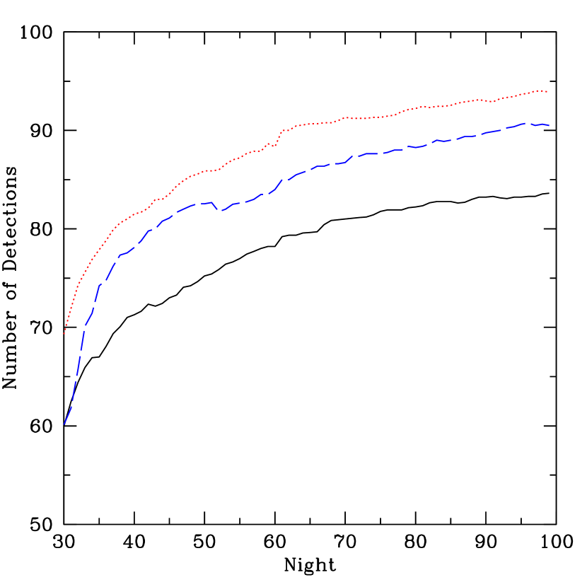
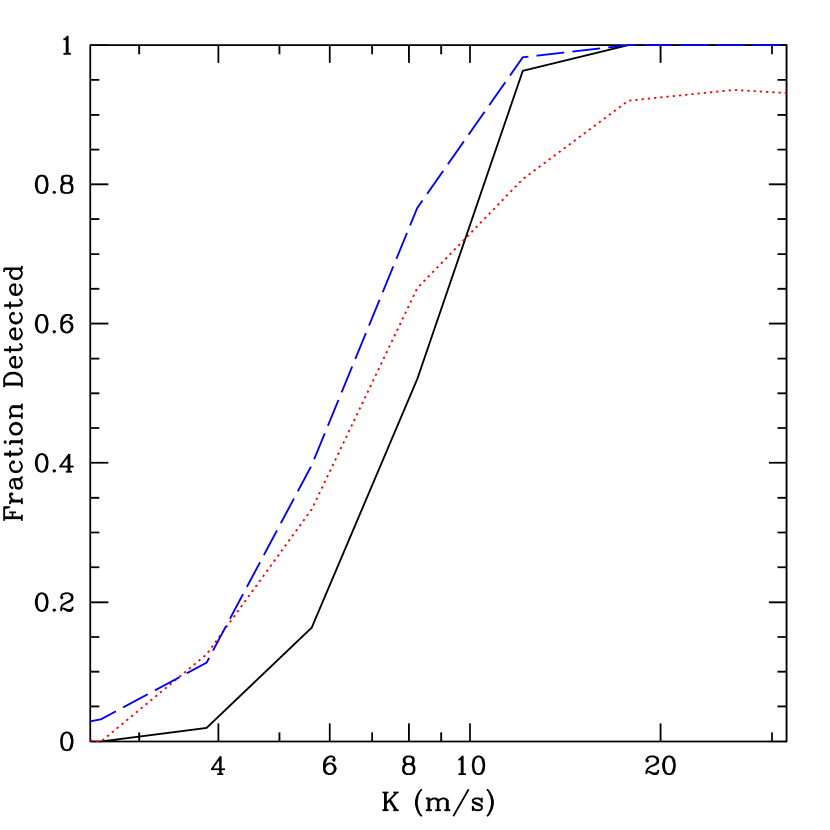
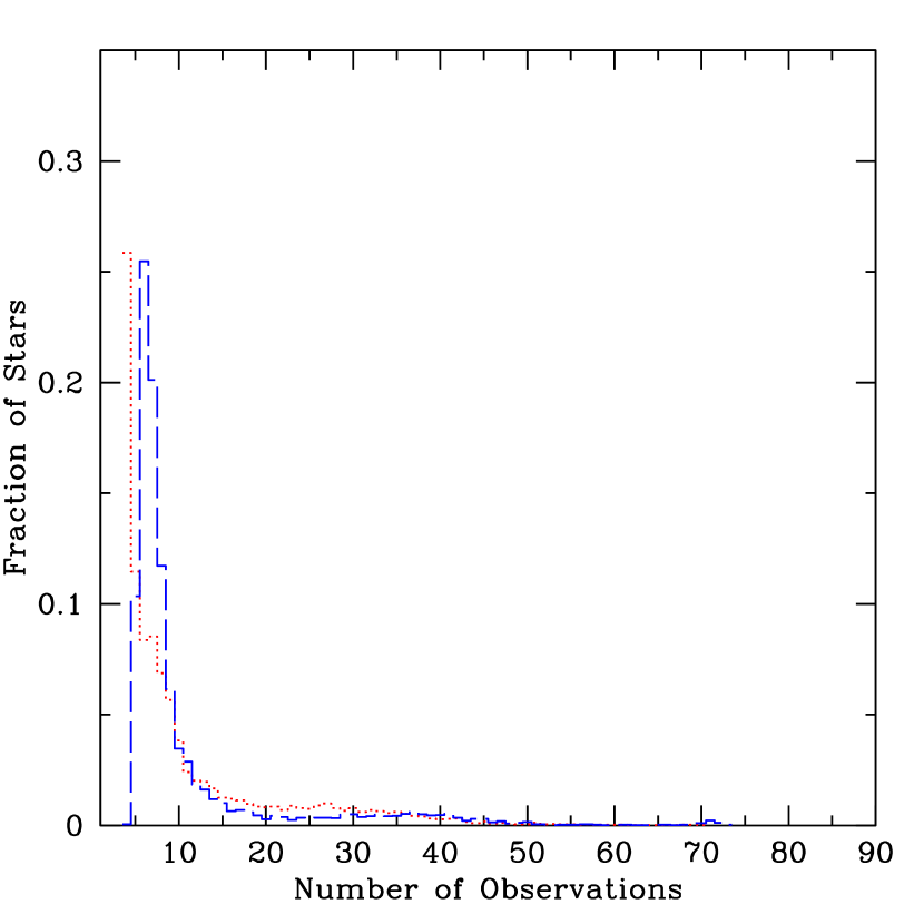
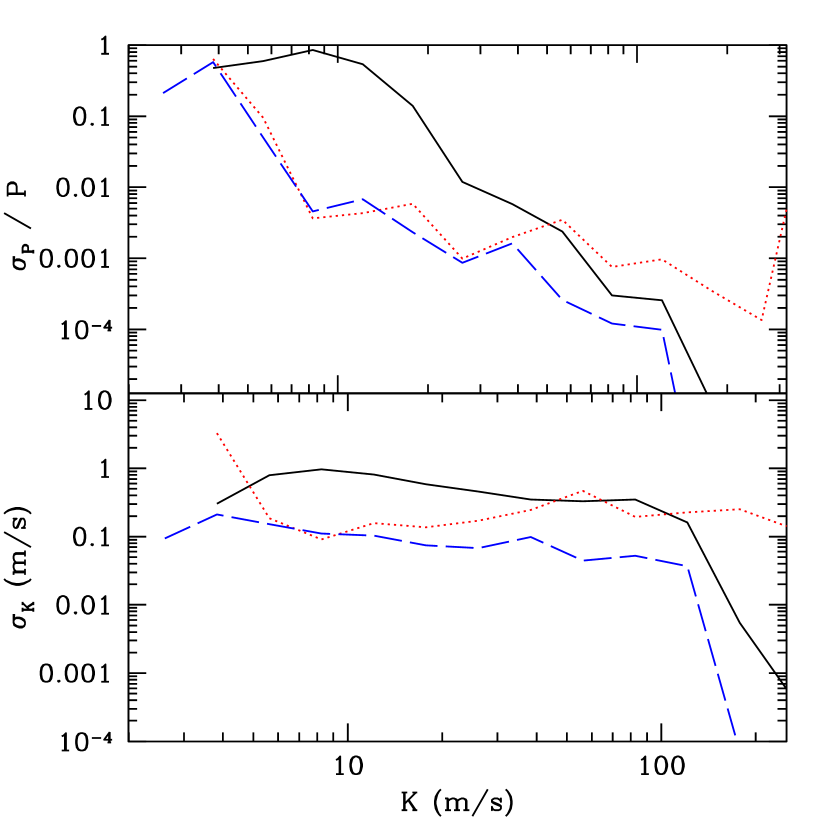
Here we present a summary of the results of these simulations. At the end of each night we monitor the posterior distributions for the model parameters of each system, paying particular attention to the number of planet detections (which we define to be systems for which the probability of the null hypothesis, no planet, is less than 0.1%). In Fig. 2, we show how the number of detections increases as a function of the number of observing nights. The adaptive scheduling algorithm based on §3 (dashed blue) is clearly more efficient than the regular scheduling algorithm (solid black) for detecting planets, even though it is not explicitly optimized for detecting the largest number of planets. More importantly, the additional planets that are being detected by the adaptive scheduling algorithm, tend to be those with the smallest velocity amplitudes (see Fig. 3). This is accomplished by observing some stars more frequently than others. In Fig. 4 we present a histogram showing the fraction of stars that were observed a given number of times. While the regular scheduling algorithm observed each star ten times, the adaptive algorithms observed many stars slightly less frequently and a few stars much more frequently. This makes the adaptive scheduling algorithms much more sensitive to planets with velocity amplitudes near the threshold of detection. Thus, while the total number of planets detected increases by $\sim 10-20\%$, the mass of the least massive planet detected by the adaptive scheduling algorithm is less than that of the regular scheduling algorithm by a factor $\sim 2$ or more. It is also important to note that the accuracy with which the orbital parameters are measured has not been sacrificed (see Fig. 5). While the orbital periods and amplitudes for planets with the largest velocity amplitudes ($\geq 100$m/s) are measured with a similar accuracies, the adaptive scheduling algorithm provides a significant improvement in the accuracy of the orbital parameter determinations for planets with more modest velocity amplitudes ($\leq 30$m/s).

4. Alternative Utility Functions

In §2 we focused on when to observe a single star, and hence the predictive distribution, $p(v|\vec{d})$, and its entropy were an obvious choices for comparing the utility of observations at various times. In §3, we focused on choosing which star (from a large list) should be targeted at the next observing opportunity. In §3, we choose a utility function based on the joint posterior for the model parameters for all the target stars. However, in this case the choice of utility function is less obvious. Various surveys and investigators may have differing goals and hence differing utility functions. For example, one possible goal would be to measure the orbital parameters to some desired accuracy. Another reasonable goal might be to discover as many planets as possible given some fixed amount of observing time. In that case, it would make sense to stop observing stars once it had been established that they harbored a planet, even if the orbital elements were not yet well constrained. An even more extreme example is for a radial velocity survey intended to help select reference stars for astrometric survey by future missions such as SIM. In that case, one could stop observing a star before obtaining a rough measure of the orbital parameters or even before the false alarm rate (for detecting a planet) was small. This is similar to a strategy for a survey aimed at discovering planets with a small mass which would eliminate stars once the radial velocities are observed to vary over too large a range to be due to a low mass planet. Yet another possible goal would be to discover multiple planet systems or planets with long orbital periods. In this case, one would not want to stop observing a star even after the orbit of one planet had been well characterized, if it was still possible the system could have an additional planet with a longer orbital period.

The above examples illustrate that simply targeting stars based on the maximum entropy method with the same utility function is not always the best strategy for a given application. Nevertheless, we have demonstrated that adaptive scheduling algorithms can significantly increase the efficiency of an observing program. Thus, it is important that the goals of an observing program be carefully considered and clearly identified. Then, a utility function can be chosen that is appropriate for the particular purpose of the observations. Once a utility function has been defined, the methods outlined in this paper can be used to optimize the observing program for the given utility function.

The utility function discussed above, $E\left[\Delta I\left\{p(\vec{m}|\vec{d}^{\prime})\right\}\right]$, is relatively easy to calculate based on the posterior distribution, $p(\vec{m}|\vec{d})$, giving it a practical advantage over many other possible utility functions. In this section we describe simple generalizations of the above utility function which are can be computed with a similar efficiency. The generalized maximum entropy utility functions that we describe below provide a means for optimizing observing schedules for a broad range of goals.

4.1. Information about a Subset of Models

One case worth considering is when we are only interested in models which satisfy certain criteria. For example, we might only be interested in obtaining more information about stars with planets (and not about the constant velocity of stars without planets). Similarly, we might be interested in companions with (minimum) masses less than some threshold, perhaps to exclude binary stars or perhaps to target terrestrial-mass planets. In this case we could replace $I\left\{p(\vec{m})\right\}$ with

$$I_{\Theta}\left\{p(\vec{m})\right\}=\int d\vec{m}\,p(\vec{m})\theta(\vec{m})\log p(\vec{m}),$$ (30)

where $\Theta$ is a region of the model parameter space, $\theta(\vec{m})=1$ when the parameters $\vec{m}$ satisfy a certain criteria and $\theta(\vec{m})=0$ otherwise. The expression for $I_{\Theta}(p(\vec{m}))$ can be thought of as the information contained in the distribution $p(\vec{m})$ about the subset of model parameters in $\Theta$. In this case, the relevant utility function becomes

$$E\left[\Delta I_{\Theta}\left\{p(\vec{m}|\vec{d}^{\prime})\right\}\right]=p(\vec{m}\in\Theta)I\left\{p(v|v_{actual})\right\}-\int d\vec{m}\,p(\vec{m}|\vec{d})\theta(\vec{m})\int dv\,p(v|\vec{m})\log\left[p(v|\vec{d})\right],$$ (31)

where the first term is again a constant, provided that the scale and shape of the sampling distribution does not depend on the model parameters.

In the above example, we used $\theta(\vec{m})$ as an indicator variable to specify when the parameters satisfied some criteria of interest, such as whether the model includes a planet or whether the orbital period is less than some threshold. More specialized forms of $\theta(\vec{m})$ could be chosen for specific goals, such as finding planets with certain orbital periods (e.g., within the habitable zone). In principle, $\theta(\vec{m})$ could be used as a weight, specifying the relative value of information about systems with various model parameters. For example, a planet search aiming to discover low-mass planets could specify a $\theta(\vec{m})$ which decreases for high mass planets.

4.2. Information in Marginal Distributions

Another case worth considering is when some model parameters are of more scientific interest than others. For example, the constant stellar velocities, $C_{0}$ and $C_{1}$, contain no information about extrasolar planets. Similarly, the angle $\phi_{o}$ may be of less interest than other model parameters such as the orbital period, $P$. As an extreme example, one might be interested in determining only if a star has a planet and not be interested in measuring the orbital parameters. In such cases, it is useful to subdivide the set of model parameters, $\vec{m}$, renaming them $(\vec{m},\vec{n})$, where $\vec{m}$ is the set of scientifically interesting model parameters and $\vec{n}$ is the set of “nuisance” parameters. Now, we can marginalize over the nuisance parameters and consider the expected change in the information contained in the probability distribution, $p(\vec{m}|\vec{d}^{\prime})=\int dnp(\vec{m},\vec{n}|\vec{d}^{\prime})$, rather than using the joint distribution $p(\vec{m},\vec{n}|\vec{d}^{\prime})$ as before. Thus, the relevant utility function becomes

$$E\left[\Delta I\left\{p(\vec{m}|\vec{d}^{\prime})\right\}\right]=\int d\vec{m}\,p(\vec{m}|\vec{d})\int d\vec{n}\,p(\vec{n}|\vec{d},\vec{m})\int dv\,p(v|\vec{m},\vec{n})\log\left[\frac{\int d\vec{n}^{\prime}p(\vec{n}^{\prime}|\vec{d},\vec{m})p(v|\vec{m},\vec{n}^{\prime})}{\int d\vec{m}^{\prime}\int d\vec{n}^{\prime}p(\vec{m}^{\prime},\vec{n}^{\prime}|\vec{d})p(v|\vec{m}^{\prime},\vec{n}^{\prime})}\right].$$ (32)

Here the first two integrals sample over all possible models and the third integral samples over all possible values of the observed velocity, just as before (e.g., Eqn. 24). Indeed, if the logarithm were split into the difference of two terms, then the term arising from the denominator would also be mathematically equivalent to the (negative of) Eqn. 24. However, the term arising from numerator causes this utility function to differ from Eqn. 23, as it no longer simplifies to equal the information of the upcoming observation if the actual velocity were known. For the utility function in Eqn. 23, the entropy of the predictive distribution at the time of a hypothetical future observation is compared to the entropy of the probability distribution for the observed value given the actual value. However, for this choice of utility function, the entropy of the predictive distribution at the time of a hypothetical future observation is compared to the entropy of the predictive distribution marginalized over the nuisance parameters (evaluated for the same time). Thus, both terms depend on the time, and a hypothetical future precise observation would be expected to contribute less information at times where the predictive distribution is more sensitive to the values of the nuisance parameters.

If we marginalize over all the fit parameters, then we can obtain posterior distributions for the probability that the system does or does not have a planet. A scheduling algorithm based on maximizing the expected increase in information contained in this distribution is expected to detect planets very efficiently. Indeed, we can see that this is the case from the dotted red curve in Figs. 2 & 3.

4.3. Non-Greedy Algorithms

So far we have restricted our attention to “greedy” algorithms, since the utility functions have only considered the effect of a single additional observation (Cormen et al. 2001). As we have demonstrated, these greedy algorithms perform quite well in the cases which we considered. However, it is worth briefly discussing alternative “non-greedy” utility functions.

Let us consider the case where making one additional observation is expected provide no or little increase in information, but making multiple additional observations (perhaps at particular times) would be expected to provide significant additional information. A simple example of such a situation is when a new target star is added to the survey. The first two observations of any star can not result in the detection of a planet. Yet, if the current target list has been searched thoroughly, then it could be more productive to add new stars to the target list. While this effect is increased when the constant velocities are considered nuisance parameters, there is some effect even when $C_{0}$ and $C_{1}$ are considered parameters of interest.

In principle, cases such as these can be handled by calculating the expected increase in information at some later time by which several additional observations could be made. Multiple additional observations are considered by sampling over the various possible combinations of future observations. This generalization has the obvious drawback that it is necessary to perform an additional integral over various possible combinations of observing schedules. One possible simplification is to relax the assumption that the total number of observations is held fixed (only for the purpose of evaluating the integral over future observing schedules) and to consider observing schedules for each star separately. Then the integral over future observing schedules can be performed separately for each star by assuming a constant probability of making an observation at each possible future observing time.

In principle, the above algorithm could identify combinations of multiple observations which are significantly more valuable than would be estimated by a greedy algorithm. Another benefit of the above algorithm is that it can automatically account for differences in the fraction of time during which stars are observable (e.g., due to seasonal effects). We have performed a few small simulations using the non-greedy algorithm described above and found that they provided a small increase in observing efficiency for the cases which we considered. However, a through comparison of greedy and non-greedy algorithms will require significantly more computation power.

4.4. Utility Functions with Costs

The utility function can also include information about the cost of making a given observation. While economic cost is often used in Bayesian decision theory, for our applications it is preferable to use observing time necessary to perform an observation as the measure of cost. The observing time required for a given observation includes the time necessary to collect the desired number of photons, but also the time required for CCD readout and slewing the telescope from the previous target to the next target. The time required for CCD readout is known and a constant for each exposure. (For faint target stars, it may be necessary to use multiple exposures for a single observation, if the barycentric correction would vary significantly during the necessary integration time.) For target stars near the previous target, the telescope can often slew to the target during CCD readout, resulting in no or minimal loss of observing time to slewing. Typically, observing schedules within a night are chosen so that the vast majority of the observing time is spent integrating on targets. The main factor in determining the integration time necessary is the apparent magnitude of the target star. In principle, adaptive scheduling algorithm could plan an entire evenings observations, considering the cost to observe each possible target throughout the night. However, the exact amount of integration time depends on the atmospheric extinction (which we assume in proportional to the airmass) as well as time variable atmospheric conditions that are generally not known in advance. Therefore, we do not believe that it is worthwhile to include such a fine level of scheduling when selecting targets for a given night. In practice, atmospheric conditions (e.g., seeing and cloud cover) change throughout a night, making it impossible to know in advance the number of targets that can be observed during that night. Given the computational complexity of these algorithms, it is impractical to perform new analyzes throughout the night as atmospheric conditions change. By assuming that atmospheric extinction is a function of airmass only (e.g., ignoring the possibilities of cloud cover or atmospheric conditions changing throughout the night), we can compute the expected amount of observing time necessary for each possible target star. Then, we identify the targets with the greatest expected increase in information per unit observing time (rather than per observation).

5. Discussion

We have developed a practical algorithm for applying adaptive scheduling to radial velocity planet searches. The algorithms presented are rigorously grounded in Bayesian data analysis and information theory, and still permit specialization for the specific goals of the observing program. While such adaptive scheduling algorithms are computationally demanding, they can provide dramatic benefits. Already, there is some element of “adaptive” scheduling due to human feedback (e.g., observers identify interesting targets to be observed more frequently, time allocation committees decide how much and when observing time will be made available). Unfortunately, quantifying these effects is extremely difficult. One advantage of following an algorithmic procedure is that any biases can be recognized, simulated, and quantified.

As we demonstrated in Fig. 2, the use of adaptive scheduling algorithm can significantly increase the number of planet detections in a survey with a fixed amount of observing time. Perhaps, more significantly, the additional planets found tend to have the smallest velocity amplitudes and hence smaller masses of those detected in the survey, as seen in Fig. 3. For the survey parameters which we considered, we found the least massive planet being detected in a survey is a factor $\sim 2$ less massive when using our adaptive scheduling algorithms than when scheduling observations randomly. It is important to appreciate that the increased the number of planet detections does not require reducing the precision of measurements of orbital parameters. In fact, the same algorithms which increase the number of planet detections simultaneously can improve the precision with which most of orbital parameters are measured (Fig. 5). While the precision is comparable for planets with very large velocity amplitudes, for low mass planets the adaptive algorithms typically measure orbital parameters with more than an order of magnitude smaller uncertainties.

The adaptive algorithms presented in this paper address several important challenges raised by previous studies. In this paper, we dramatically reduce the computational requirements for Bayesian adaptive scheduling algorithms relative to Loredo (2004). We accomplish this by separating the integrals over orbital period from the integrals over the other orbital parameters. By assuming planets on circular orbits, the remaining integrals become Gaussian integrals which can be evaluated analytically. The increased efficiency has made several other advances possible. The increased computational efficiency of our algorithms allows us to conduct Monte Carlo simulations of entire planet search programs and quantify the increase in efficiency that adaptive scheduling algorithms offer. More significantly, our algorithms make it practical to perform a Bayesian analysis of the orbital parameters even when there are extremely weak constraints on the orbital parameters, such as when only a few observations have been made. This has allowed us to apply Bayesian hierarchical modeling to simultaneously consider both possibilities that a star has no planet and that the star has one planet, extending previous Bayesian techniques which assumed there was a single planet (Loredo 2004; Ford 2005, 2006). By constructing hierarchical models, adaptive scheduling algorithms naturally consider the problems of planet detection and orbital parameter estimation simultaneously. We also present several generalizations of our computationally efficient algorithms. The generalized algorithms can accommodate a variety of utility functions which can be customized to the specific goals of an observational program. These generalizations also allow the adaptive scheduling algorithm to consider practical complications such as stars of different brightnesses and observing seasons.

This work also raises several new challenges. Clearly, it would be desirable to generalize our algorithms to reflect the full variety of planetary systems. For example, we assume that each star has a maximum of one planet, while there are already $\sim$12 stars known to have multiple planets. In principle, it is easy to generalize our hierarchical models to allow more multiple planets, but in practice each additional planet would introduce an additional integral which can not be evaluated analytically and dramatically increase the required computations.

Additionally, we have assumed circular planetary orbits, while most extrasolar planets have significant eccentricities. We have conducted some simulations in which we consider a population of stars with planets on eccentric orbits but the adaptive scheduling algorithm assumes circular orbits. While the adaptive scheduling algorithms still detect planets and measure orbital parameters more efficiently than non-adaptive algorithms, the improvement in efficiency is less than when applied to a population of stars with planets on circular orbits. Intuitively, we expect that planets on eccentric orbits could benefit from adaptive scheduling algorithms even more than planets on circular orbits. Therefore, we expect that the reduction in efficiency is due to the adaptive scheduling algorithm not having access to the appropriate model. Again, in theory, it is straightforward to include eccentric orbits in a Bayesian analysis, but this would introduce an additional two integrals which can not be evaluated analytically and hence would significantly increase the require computations. Incorporating eccentric orbits into adaptive scheduling algorithm could be accomplished by brute force, or it might be sufficient to use approximate models which expand the orbital motion in the eccentricity.

Our simulations have also assumed that planetary perturbations are the only cause of variations in the star’s radial velocity. In practice, many stars appear to have intrinsic variability commonly known as stellar “jitter” which can be comparable to or exceed the observational uncertainties in the radial velocity measurements (Saar, Butler, & Marcy 1998). We have conducted some simulations in which we consider a population of stars where each star has a Gaussian jitter, but the adaptive scheduling algorithm assumes no jitter. The primary effect of the jitter is to increase the false alarm rate (fraction of stars with no planets for which the Bayesian analysis determines the probability of having no planet is less than 0.1%). While the threshold for announcing a planet detection can be altered to maintain a 0.1% false alarm rate, such a treatment is simplistic and does not properly account for the unknown jitter. The problems posed by jitter can be mitigated by replacing the observational uncertainties with the observational uncertainties added in quadrature to the amount of jitter expected based on the star’s spectral properties. Still, this approach could result in poor performance when the estimate for the stellar jitter is inaccurate. Indeed, one of the advantages of Bayesian analysis is that it can naturally allow for noise sources of unknown magnitude. A more rigorous analysis would treat the stellar jitter of each star as an unknown along with the orbital parameters. Unfortunately, adding the stellar jitter as a model parameter introduces an additional integral and requires additional computation time. For the purpose of testing adaptive scheduling algorithms when confronted with jitter, it may be useful to consider a special case in which the observational uncertainties are the same for each observation. In this case, the integral over the unknown stellar jitter can be performed separately from the other integrals and reduces to a sum of exponential integrals which can be performed analytically (Cumming 2004).

This paper has focused its attention on adaptive scheduling algorithms for radial velocity planet searches. Targeted astrometric planet searches such as those planned for the Space Interferometry Mission (SIM) are another obvious application of our methods. Given the cost and finite lifetime of space missions such as SIM, observing time is extremely valuable and it is even more important to make the best use of the available observing time. Successfully incorporating Bayesian adaptive design would require that the observation schedule not be fixed far in advance by logistical constraints. Mission designers should aim to allow for frequent upload of revised target lists. In principle, the two types of planet searches are quite similar, with the main difference that astrometric surveys can measure the stellar position in two dimensions while radial velocity surveys can measure the stellar velocity in only one dimension. Therefore, we expect that adaptive scheduling algorithms could also provide a significant improvement in the efficiency of the SIM planet searches, resulting in more planets being discovered, planet masses and orbital parameters being determined more accurately, and significantly increasing the sensitivity of SIM to nearly-Earth-mass planets and multiple planet systems. For this potential benefit to be realized the SIM design must be sufficiently flexible that the observing schedule and target stars can be chosen with a lead time much less than the duration of the mission, preferably a lead time of a month or less. To fully simulate such an adaptive scheduling algorithm, it will be important to incorporate the practical observing constraints and costs (e.g., possible pointing directions limited, time require to slew to different positions).

Figure 1.— Here we show the expected value for the radial velocity (solid line) during October and November 2004 (tick marks very five days) of four different target stars from the N2K project. The dotted lines show the 95% confidence intervals for $p(v|d)$ as a function of time. These predictive observations were based on observations taken between January 10 and July 11, 2004 (not shown) as a part of the N2K survey. The arrows near the bottom of each panel indicate the time when the entropy of the predictive distribution is maximized. The arrows near the bottom of each panel indicate the time when the standard deviation of the predictive distribution is maximized. The predictive distributions are based on 4 (top left), 5 (top right), 11 (bottom left), and 6 (bottom right) observations. The best-fit orbital periods are near 53d (top left), 52d (top right), 16 d (bottom left), and 27d (bottom right).

Figure 2.— Here we show the expected change in the expectation of the information content following a single observation as a function of the time, $t$ (dotted line). This is to be compared to the log of the standard deviation of the predictive distribution (solid line). The figure is based on the first five of the observations of HD 88133, the first planet discovered by the N2K project (Fischer et al. 2004). The times of the observations are indicated with vertical arrows. While the two curves show similarities, the most/least favorable times according to an information theory analysis are not always coincident with what would be predicted using only the variance of the predictive distribution.

Figure 3.— This figure shows the number of planets detected (stars for which the posterior probability of the no-planet model, $p(0|\vec{d})$, is less than 0.1%) as a function of the number of observing nights. The different line styles present the results for different scheduling algorithms: regular (solid black), the adaptive algorithm from §3.1 (dashed blue), and the adaptive algorithm from §4.2 (dotted red), which maximizes the detections at the expense of accuracy in orbital parameters by marginalizing over orbital parameters (compare to Fig. 5). The results for each scheduling algorithm have been averaged over ten simulated observing programs.

Figure 4.— Here we show the fraction of planets detected as a function of the velocity semi-amplitude, $K$. In these simulations each observation had an observational uncertainty of $\sigma_{\mathrm{o}bs}=3$m/s. The planet searches based on both adaptive algorithms are significantly more efficient at detecting planets with $K\sim 1-3\sigma_{\mathrm{o}bs}$ than the fixed schedule (solid black line). The line styles are as in Fig. 2.

Figure 5.— In this figure we present a histogram of the number of time a star was observed. For the regular scheduling algorithm, each star was observed ten times (not shown). The adaptive algorithm from §3.1 (dashed blue) and the adaptive algorithm from §4.2 (dotted red) both devote a large number of observations to a few stars, significantly increasing the sensitivity to low-mass planets around these stars.

Figure 6.— Here we show the median precision of the measurements of the orbital parameters, $P$ (top panel) and $K$ (bottom panel), as a function of the velocity semi-amplitude, $K$. Both adaptive scheduling algorithms typically perform significantly better than the fixed schedule (solid black line). However, for large velocity amplitudes, the adaptive algorithm presented in §3.1 often allocates a only small number of observations to planets with large velocity amplitudes and hence the orbit determinations are not as precise as with the fixed schedule. The line styles are as in Fig. 2.

References

- (1) Cormen, T.H., Leiserson, C.E., Rivest, R.L., Stein, C. 2001 Introduction to Algorithms. (Cambridge, MA: MIT Press)
- (2) Cumming, A., Marcy, G.W., Butler, R.P., & Vogt, S.S. 2002, in “Scientific Frontiers in Research on Extrasolar Planets” eds. D. Deming & S. Seager; ASP Conferences Series 294, 27.
- (3) Cumming, A. 2004 MNRAS, 354, 1165.
- (4) Endl, M., Kurster, M., Els, S., Hatzes, A.P., Cochran, W.D., Dennerl, K., Dobereiner, S. 2002 A&A 392, 671.
- (5) Fischer, D.A., Laughlin, G., Butler, R.P., Marcy, G.W., Johnson, J., Henry, G., Valenti, J., Vogt, S.S., Ammons, M., Robinson, S., Spear, G., Strader, J., Driscoll, P., Fuller, A., Johnson, T., Manrao, E., McCarthy, C., Munoz, M., Tah, K.L., Wright, J., Ida, S., Sato, B., Minniti, D. 2005, ApJ, 620, 481.
- (6) Ford, E.B. 2004, PASP, 116, 1083.
- (7) Ford, E.B. 2005, AJ, 129, 1706.
- (8) Ford, E.B. 2006, ApJ, 642, 505.
- (9) Gaudi, B.S., Seager, S., Mallen-Ornelas, G. 2005, ApJ, 623, 472.
- (10) Konacki, M., Torres, G., Saurabh, J., Sasselov, D. 2003, Nature, 421, 507.
- (11) Loredo, T.J. 2004, in “Bayesian Inference And Maximum Entropy Methods In Science And Engineering: 23rd International Workshop” ed. G. J. Erickson and Y. Zhai; AIP Conference Proceedings 707, 330.
- (12) Pourbaix, D. 2002, A&A, 385, 686.
- (13) Rasio, F.A., Tout, C.A., Lubow, S.H. Livio, M. 1996, ApJ, 470, 1187.
- (14) Saar, S.H., Butler, R.P., Marcy, G.W. 1998, ApJ, 498, 153.
- (15) Sivia, D.S. 1996 Data Analysis: A Bayesian Tutorial. (New York, NY: Oxford University Press)
- (16) Sozzetti, A., Casertano, S., Brown, R.A., Lattanzi, M.G. 2002, PASP, 114, 117.
- (17) Tabachnik, S. & Tremaine, S. 2002, MNRAS, 335, 151.
- (18) Udry, S., Mayor, M., Clausen, J., Freyhammer, L., Helt, B., Lovis, C., Naef, D., Olsen, E, Pepe, F., Queloz, D., Santos, N. 2003, A&A, 407, 679.