Recent Results from the EVN Mk IV Data Processor at JIVE

Abstract

Recent achievements at the EVN Mk IV data processor at JIVE include decreasing the read-out time for the whole correlator to 0.25 s (or 0.125 s for half the correlator), improving the end quality of user data (e.g., applying an improved 2-bit van Vleck correction), developing new astronomical capabilities (e.g., oversampling to $\times 4$, wider-field mapping), and strengthening liaison procedures with PIs (e.g., pipelining, the EVN Archive facility). At the same time, the move to a disk-based EVN and regular incorporation of FTP fringe-checks is well underway, resulting in more reliable data quality. We will review these developments, highlighting how they may broaden the kinds of astronomy you can do. We’ll also go over some measures you can take to help you get the most out of these new/improved features.

1 Background

A key item in the Mk IV upgrade of the EVN was the construction of the EVN Mk IV data processor at the Joint Institute for VLBI in Europe (JIVE). JIVE is hosted by ASTRON in Dwingeloo, the Netherlands, and is funded by science councils of a number of European countries. Special projects have been funded directly by the European Commission. The EVN Mk IV data processor was constructed in the context of the International Advanced Correlator Consortium through which the other Mk IV geodetic correlators were also built, with significant contributions from European partners (Casse [1999]; Schilizzi et al. [2001]).

The first fringe on the EVN Mk IV data processor was seen on 21 July 1997 and its official inauguration took place on 22 October 1998. The EVN Mk IV data processor now correlates the vast majority of astronomical EVN experiments, and about half of the global experiments. Altogether, we have processed 175 user and 116 network/test experiments as of 9 September 2004.

Here, we will concentrate on areas of interest to the user having data correlated at JIVE: tools for planning observations with regard to the data processor’s increased capabilities, current operational and communication flow between JIVE and the PI, and services you can call on at JIVE to help you get the most out of your observations. More information about the EVN and JIVE can be found at the websites www.evlbi.org and www.jive.nl.

2 Current Capabilities

The EVN Mk IV data processor can correlate simultaneously up to 16 stations with 16 channels per station, each having a maximum sampling rate of 32 Ms/s (thus a total of 1 Gb/s per station for 2-bit recordings). The correlator houses 32 Mk IV boards. The principal science drivers behind the development of the data processor and associated software include the ability to handle continuum dual-polarization observations, spectral line experiments, and phase-reference mapping.

2.1 Features Snapshot

The EVN Mk IV data processor can currently correlate/provide:

1. 1- and 2-bit sampling (all but a handful of experiments use 2-bit sampling).

2. Mk III, Mk IV, VLBA, and Mk5(A) recordings.

3. sustained 512 Mb/s tape recordings or 1 Gb/s for Mk5 disk recordings.

4. parallel- and cross-hand polarization products as desired in dual-polarization observations.

5. up to 2048 frequency points per interferometer (i.e., each baseline/subband/polarization — see the discussion following equation (1) below).

6. full-correlator integration times down to 0.25 s (half-correlator $t_{\rm int}$ down to 0.125 s).

7. oversampling at 2 or 4 times the Nyquist frequency, in order to provide subband bandwidths down to 500 kHz (the maximum Nyquist-sampled $BW_{\rm sb}$ is 16 MHz).

8. multi-pass correlation (e.g., for observations having $>$16 stations at any given time).

9. an improved 2-bit van Vleck correction to account for the statistics of high/low bits for each IF’s data stream from each station.

Capabilities whose development are still underway or not yet fully tested include pulsar gating, speed-up (playback at a bit-rate faster than used in recording), and phase-cal extraction. Capabilities that are yet to come include sub-netting (although we can manually handle the set-ups for reasonably straightforward instances) and recirculation (achieving greater equivalent correlator capacity, through a time-sharing scheme, for observations that don’t use the maximum bandwidth per subband).

2.2 Correlator Capacity

The total correlator capacity can be expressed as:

$$N^{2}_{\rm sta}\cdot N_{\rm sb}\cdot N_{\rm pol}\cdot N_{\rm frq}\leq 131072$$ (1)

Here, $N_{\rm frq}$ is the number of frequency points per interferometer (baseline/subband/polarization). $N_{\rm pol}$ is the number of polarizations in the correlation (1, 2, or 4). $N_{\rm sb}$ represents the number of different subbands, counting lower- and upper-sidebands from the same BBC as distinct subbands. The value to use for $N_{\rm sta}$ is “granular” in multiples of 4: for example, if you have 5–8 stations, use “8”. Independent of this equation, the maximum number of input channels ($N_{\rm sb}\cdot N_{{\rm pol}_{\parallel}})$ is 16, and the maximum $N_{\rm frq}$ is 2048 (a single interferometer must fit onto a single correlator board). The minimum $N_{\rm frq}$ is 16. On a more technical note, all capabilities discussed in this report assume the use of local validity, which avoids problems arising from Mk IV-format data-replacement headers correlating against each other in certain baseline-source geometries, but does so at the expense of a factor of two in $N_{\rm frq}$.

$N_{\rm sta}$	$N_{\rm sb}$	$N_{\rm pol}$	$N_{\rm frq}$	comment
8	1	1	2048	EVN spectral-line
9	1	1	512	9th sta: $N_{\rm frq}\rightarrow N_{\rm frq}/4$
16	8	4	16	global cross-polarization
16	2	2	128	re-arrange $\{N_{\rm sb},N_{\rm pol},N_{\rm frq}\}$
8	16	1	128	How $N_{\rm sta}$ increase can be
12	7	1	128	absorbed by $N_{\rm sb}$
16	4	1	128	(not constrained to be $2^{n}$)

Table 1: Examples of “maximal” correlator configurations (local validity).

2.3 Output Capacity

The minimum $t_{\rm int}$ for a configuration using the whole correlator is now $1/4$ s; configurations that use no more than one-half of the correlator can achieve a minimum $t_{\rm int}$ of $1/8$ s. In the near future, the development of the Post-Correlator Integrator (PCI) aims to provide a minimum $t_{\rm int}$ for the whole correlator of $1/64$ s.

These low integration times, together with the fine spectral resolution afforded by large $N_{\rm frq}$, will provide the possibility to map considerably wider fields of view through reduced bandwidth- and time-smearing effects in the u-v plane (see, e.g., Bridle & Schwab [1989]; Wrobel [1995], § 21.7.5). For example, the fields of view having $\leq 10\%$ decrease in the response to a point source arising from each of these two effects are:

$$FoV_{\rm BW}\stackrel{{\scriptstyle{\textstyle<}}}{{\sim}}49.\!^{\prime\prime}5\,\frac{1}{B}\,\frac{N_{\rm frq}}{BW_{\rm sb}};\quad FoV_{\rm time}\stackrel{{\scriptstyle{\textstyle<}}}{{\sim}}18.\!^{\prime\prime}56\,\frac{\lambda}{B}\,\frac{1}{t_{\rm int}}$$ (2)

Here, $B$ is the longest baseline length in units of 1000 km, $\lambda$ is in cm, and $BW_{\rm sb}$ is in MHz. A primary goal of such wide-field correlations would be to map the entire primary beam of each antenna composing the array with only a single correlation pass. With our existing $N_{\rm frq}$ and $t_{\rm int}$ capabilities, we can already achieve this for a variety of observing configurations, with time-smearing usually the limiting factor. More details can be found in www.evlbi.org/user_guide/limit.html. Of course, one potential drawback to such wide-field correlations, and the short $t_{\rm int}$ they require, is the rapid growth of the size of the FITS file seen by the user — reaching about 7 GB per hour of observation at our current maximum output rate.

3 Operational Overview

Since the previous EVN Symposium, a re-organization at JIVE has brought the Correlator Science Operations and the EVN Support Group together to form the Science Operations & Support Group. From the PI’s viewpoint, this new structure should present better integrated assistance for all segments of your experiment — from proposing/scheduling through correlation to analysis of the resulting FITS data. We are also continually upgrading our visitor computing resources, and the domain of European PIs eligible for financial support for visiting JIVE (or other EVN institutes) has been broadened as of February 2004. Both the JIVE and EVN web pages have been revised to improve the ease of navigation and the mutual cross-linking. The EVN Users’ Guide on the EVN web page (www.evlbi.org/user_guide.html) remains the best “first stop” for on-line help. It has direct links to:

1. tasks encountered in conducting EVN experiments (proposing, scheduling, correlating, analyzing).

2. the EVN Data Archive (see § 3.3).

3. travel support information.

4. handy tools & documents (the EVN calculator, the EVN data analysis guide).

5. EVN facts & figures (frequency/u-v coverage, resolution, baseline/image sensitivity, imaging limitations).

3.1 Pre-observation, Pre-correlation

Figure 1 summarizes operational and communication flow among the PI, JIVE, and various EVN assets during an EVN astronomical experiment. The first step is creation of the experiment schedule. We actively encourage the PI to consult with Science Operations & Support group at JIVE during scheduling, in order to help side-step the myriad little pitfalls that may lead to unpleasant surprises when (and after) the observations are carried out. Following the observation but prior to the correlation itself beginning, we confer with the PI to make sure the correlation parameters (e.g., $N_{\rm pol}$, $N_{\rm frq}$, $t_{\rm int}$) are appropriate and to discover any desired changes (e.g., improved source coordinates). Each experiment is assigned a support scientist, who shepherds it through the correlation and post-correlation analysis stages discussed below.

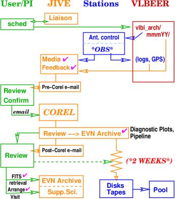
Figure 1: Operational flow for the observations and correlation of an experiment (check = item available via JIVE or EVN web pages).

3.2 Correlation and Logistics

We operate the correlator 80 hours per week, from which time system testing/development as well as network tests must also come; typically 45–60 hours per week are spent in production. Incorporation of Mk5 disk-based recordings has been increasing since their first use in the November 2003 session. We were hoping to see our first disk-only user experiments in the Oct/Nov 2004 session — when we can begin to reap the full efficiency gains inherent in disk playback (mixed observations of course proceed at the pace of the slower tapes). We have enough Mk5A playback units to handle any currently feasible observation, and maintain sufficient tape playback units to process tapes from NRAO stations in globals. In the longer term, when stations upgrade to Mk5B, the possibility exists to move away from using local validity, effectively doubling the correlator capacity as described in equation (1) and the maximum $N_{\rm frq}$ (the impact on the minimum $t_{\rm int}$ could be more complicated, depending on the stage of PCI development).

3.3 Post-correlation Data Review

Our main priority is always the quality of the data we provide to the EVN users. Our internal data review process, as illustrated in Figure 2, begins by transforming the lag-based correlator output into an AIPS++ Measurement Set (MS). From the MS, the support scientist can investigate slices of the correlation functions in both time and frequency, allowing us to detect and diagnose various problems with the recorded data or the correlation itself, and to find any scans for which re-correlation would be profitable. We can also make various plots more suited to providing feedback to the stations rather than to the PI (e.g., parity-error rates, sampler statistics). We apply various corrections to the correlated data at this stage (e.g., the 2-bit van Vleck correction), and flag subsets of the data for low weights and other known problems resulting in spurious correlation amplitudes and/or phases. Finally, we convert the final MS into FITS format, usually written to DAT tape. These FITS files can be read into (classic) AIPS directly using FITLD. At this stage, the support scientist sends e-mail to the PI describing the correlation and any points of interest noticed during our data review.

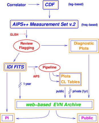
Figure 2: Post-correlation review process for an experiment.

During the course of the post-correlation review, we also begin populating the EVN Archive (www.jive.nl/archive/scripts/listarch.php) for the experiment. Feedback from the stations and the diagnostic plots from the MS-based data review go into the archive immediately to allow the PI to get an idea about the success of the correlation even before receiving the data. The standard plots typically comprise automatically generated plots of weight$(t)$ for all stations throughout the experiment, station amplitude$(\nu)$ and baseline amplitude/phase$(\nu)$ for a couple calibrator scans, and baseline amplitude/phase$(t)$ for $\sim$90 min in the vicinity of one of the calibrator scans. The FITS file(s) also go to the archive, but are kept private for a one-year proprietary period (see the EVN Data Access Policy in the EVN Users’ Guide for more details). The PI can arrange through the support scientist for a password to download the FITS data directly from the EVN Archive if desired. We are working towards providing 1 Gb/s access to the EVN Archive for the outside world.

Once we receive calibration information from the stations and process it into ANTAB files, the pipelining of the experiment can begin. The EVN Pipeline is an automated AIPS script that performs the following:

1. flags data known to be invalid (e.g., off-source).

2. applies an a priori amplitude calibration using the $T_{\rm sys}$ and gain curves from the stations.

3. fringe-fits sources authorized by the PI.

4. makes preliminary CLEAN images of these sources using a fixed scheme for phase and amplitude self-calibration.

5. creates a set of AIPS tables from various stages of the calibration/fringe-fitting process, which the PI can later apply directly to the raw data, if desired.

6. outputs a variety of intermediary plots (e.g., POSSMs, VPLOTs, dirty maps).

We ask the PI in the pre-correlation consultation how to treat each of the sources in the experiment. Pipeline results for “public” sources go directly to the EVN Archive. Pipeline results for all sources are made public after the proprietary period, along with the FITS files. The plots made in the course of pipelining provide more information with which to assess antenna performance. The resulting AIPS tables help to simplify the initial stages of the analysis. The quality of the preliminary images may be affected by the lack of interactive data editing inherent in the pipeline concept. More details about the EVN pipeline can be found in www.evlbi.org/pipeline/user_expts.html, including a link to the original pipeline paper (Reynolds et al. [2002]).

The EVN Archive is thus a central location for obtaining the information you need when reviewing/analyzing your project. Users can also query the Archive based on source names or coordinate ranges, among other characteristics, via an interface developed in Bologna. In an effort to aid citation management, we are also considering associating publications with experiments in the Archive.

Unless contacted by the PI to the contrary, we aim to release an experiment’s tapes/disks two weeks after we notify the PI of the experiment’s completion. The timely release of media for re-observation is especially important as the EVN completes its move to all-Mk5 operation. Disk procurement levels at the stations require us to ship back media in time to observe again in the next-following session. The ability of single disk-packs to cross experiment boundaries adds a potential complication: a small number of unreleased experiments may indeed tie up a disproportionately large number of disk packs. The immediate posting of station feedback and diagnostic plots to the EVN Archive endeavors to help the PI gain confidence that the correlation went well and to allay concerns about releasing the observing media.

To supplement the review products mentioned above, we encourage the PI to discuss the experiment/correlation with the responsible JIVE support scientist and/or to arrange a visit JIVE for help in data reduction if desired. In order to facilitate such visits, the eligibility of European PIs for financial support has been broadened (the bar against EVN-institute affiliation has been dropped) — see the “Access to the EVN” portion of the EVN web page for more details: www.evlbi.org/access/access.html.

4 Summary

We at JIVE are always busy working to improve the quality of the science you can achieve in your EVN or global VLBI experiments. Since the previous EVN Symposium in Bonn, these efforts have seen:

1. New astronomical capability: shorter $t_{\rm int}$ allowing wider-field mapping; oversampling to $\times$4 allowing narrower subband bandwidths and hence finer spectral resolution for a given $N_{\rm frq}$.

2. Improved correlated-data quality: a 2-bit van Vleck correction that takes into account the observed statistics of high/low bits, allowing more reliable (auto-correlation) bandpass calibration and more accurate closure amplitudes; FTP fringe tests that permit faster feedback to the stations, allowing equipment problems to be detected and repaired while the session is still underway.

3. Strengthened PI support: internal re-organization; routine pipelining; the EVN Archive; web-page redesign.