Observing Trans-Planckian Signatures in the Cosmic Microwave Background

Abstract

We examine the constraints cosmological observations can place on any trans-Planckian corrections to the primordial spectrum of perturbations underlying the anisotropies in the Cosmic Microwave Background. We focus on models of trans-Planckian physics which lead to a modulated primordial spectrum. Rather than looking at a generic modulated spectrum, our calculations are based on a specific model, and are intended as a case study for the sort of constraints one could hope to apply on a well-motivated model of trans-Planckian physics. We present results for three different approaches – a grid search in a subset of the overall parameter space, a Fisher matrix estimate of the likely error ellipses, and a Monte Carlo Markov Chain fit to a simulated CMB sky. As was seen in previous analyses, the likelihood space has multiple peaks, and we show that their distribution can be reproduced via a simple semi-analytic argument. All three methods lead to broadly similar results. We vary 10 cosmological parameters (including two related to the trans-Planckian terms) and show that the amplitude of the tensor perturbations is directly correlated with the detectability of any trans-Planckian modulation. We argue that this is likely to be true for any trans-Planckian modulation in the paradigm of slow-roll inflation. For the specific case we consider, we conclude that if the tensor to scalar ratio, $r\sim 0.15$, the ratio between the inflationary Hubble scale $H$, and the scale of new physics $M$ has to be on the order of $0.004$ if the modulation is detectable at the 2$\sigma$ level. For a lower value of $r$, the bound on $H/M$ becomes looser.

I Introduction

Conventional cosmology is based upon a four dimensional spacetime whose evolution is governed by the Einstein field equations. This picture certainly breaks down at the Planck scale due to quantum corrections to the gravitational action. Furthermore, stringy effects may change our understanding of spacetime at energies one or two orders of magnitude below the Planck scale. Unfortunately, both the Planck and string energy scales are entirely inaccessible to direct experimentation. However, thanks to the dramatic expansion of the universe during the inflationary era, it is possible that cosmology provides an unexpected window into physics at the shortest length scales Brandenberger:1999sw -Shankaranarayanan:2004iq .

If we assume the universe has always been matter dominated and is now around 13 billion years old, the current horizon size is roughly 40 billion lightyears, or $2\times 10^{61}$ Planck lengths. If inflation ended at the GUT scale ($\sim 10^{15}$GeV) with efficient reheating, the universe has grown roughly $4\times 10^{27}$ times larger since reheating, and by at least a similar amount during inflation, in order to ensure that the universe is homogeneous on scales equal to the present horizon size. Consequently, all distances significantly smaller than galactic scales in the current universe were necessarily sub-Planckian at some point during inflation. If the inflationary period continues for longer than the minimum time necessary to solve the cosmological flatness and horizon problems, all presently visible scales must have crossed the Planckian boundary during inflation. Conversely, without inflation all astrophysical scales are mapped to lengths larger than the Planck length at all times since the age of the universe was of order the Planck time.

On the face of it, the fact that astrophysical scales in the present universe correspond to sub-Planckian scales during the inflationary epoch is simply a mathematical curiosity. However, inflation generates perturbations through the exponential stretching of quantum fluctuations. The textbook calculation of the primordial perturbation spectrum implicitly ignores the consequences of the breakdown of spacetime at some new fundamental lengthscale. For a clear exposition of the standard treatment of perturbations, including a discussion of the effect of boundary conditions, see Liddlebk . In string theory the effective minimum length can be significantly larger than the Planck length, by perhaps one or two orders of magnitude Kaplunovsky:1987rp ; Arkani-Hamed:1998rs ; Antoniadis:1998ig . In this case, the ratio between the inflationary Hubble scale, $H$, and the scale of new stringy physics, $M$ can be as large as $10^{-2}$.

Dimensional analysis alone suggests that any modifications to the perturbation spectrum induced by including this minimum length will be a function of $(H/M)^{p}$, where $p$ is, of course, unknown. If $p$ is unity, then there is at least a corner of parameter space where we might expect potentially observable modifications to the spectrum. However, for larger values of $p$, any modifications to the spectrum are most likely unobservable. String theory and other candidate unified models are not sufficiently mature to permit an ab initio analysis of perturbation generation, and predict the value of $p$. Consequently, all studies of trans-Planckian modifications to the inflationary perturbation spectrum require some ansatz which, while motivated by our understanding of stringy / Planckian physics, introduces a degree of arbitrariness into the calculation. This ansatz necessarily modifies either the initial conditions or the evolution of the perturbations. Generically, modifications to the initial conditions produce changes in the spectrum on the order of $H/M$, whereas modifications to the evolution result in changes on the order of $(H/M)^{2}$. It is worth noting, however, that no calculation has predicted that the modifications vanish completely.

Normally, this lack of theoretical consensus would deter detailed studies of the observational consequences of any given model of trans-Planckian physics. However, even a small possibility that the fingerprints of Planckian or stringy physics can be found on the sky provides more than enough motivation for us to take a careful look at what constraints can be established with present data or future measurements. In this paper, we focus on one model of trans-Planckian physics, first suggested by Danielsson in the case of de Sitter space Danielsson:2002kx and generalized to non-de Sitter backgrounds by Easther, Greene, Kinney and Shiu Easther:2002xe . There is nothing intrinsically special about this model – our analysis is effectively a case study of what might be achieved when one has a specific model to test. In particular, we do not enter into the debate as to whether or not such “truncated $\alpha$-vacua” are self-consistent with respect to being well-defined in the ultraviolet limit or with respect to their suitability as initial conditions for inflation. We simply consider the model as a reasonable case study for investigating the discriminatory power of forthcoming CMB observations.

The one general statement we can make is that it is far more likely that trans-Planckian effects will have an observable impact on the spectrum if inflation takes place at a relatively high energy scale. In principle, inflation can occur at almost any scale high enough to allow for baryogenesis and nucleosynthesis in the post-inflationary universe – and this can be far below the GUT scale. However, since we only expect a detectable signal if $H/M$ is comparatively large, we are pushed into the corner of parameter space where $M$ is small (compared to the Planck scale) while $H$ is roughly GUT-scale. A small $M$ (two orders of magnitude below the Planck scale, say) is entirely consistent with string theory, whereas $H$ is effectively a free parameter. An upper bound on $H$ arises from the limits on the tensor component to the primordial perturbation spectrum – which is potentially observable via both the temperature anisotropies in the CMB, and the B-mode of the CMB polarization. (A rough upper limit on $H$ from the WMAP data is $H<6\times 10^{14}\ {\rm GeV}$.) It is very easy for inflation to happen at a low enough scale to ensure that a primordial tensor spectrum is effectively unobservable by any conceivable experiment Lyth:1996im ; Knox:2002pe ; Kesden:2002ku ; Seljak:2003pn . However, if we were to observe a contribution to the CMB that appears to be related to Planckian or stringy physics, there is a strong likelihood that we would be in the region of parameter space where $H$ was large enough in order to ensure that the tensor contribution was also detectable.

There are important consequences to this qualitative correlation between trans-Planckian contributions to the CMB and the tensor perturbations. First, it further raises the stakes for high precision measurements of the CMB. We already know that an observable tensor spectrum fixes the inflationary energy scale and rules out some of inflation’s competitors, such as the ekpyrotic Khoury:2001wf and pre-Big Bang scenarios Gasperini:1992em ; Lidsey:1999mc , and that single field models of inflation must satisfy a set of consistency conditions Lidsey:1995np . However, on top of these achievements, determining $H$ would let us put direct constraints on the scale of new physics in any specific model of trans-Planckian physics, since $M$ would be the only remaining free parameter. If $H$ turns out to be at the high end of the permitted range, it increases the likelihood that we will be able to see any trans-Planckian signal that is there to be found. Finally, one us [RE] recently argued that a high value of $H$ during inflation is naturally correlated with a scalar spectrum with a significant running index ($dn_{s}/d\ln{k}\neq 0$) Easther:2004ir . We do not consider models with substantially broken scale invariance in this paper, but do incorporate a non-zero running into our analysis below.

From a practical perspective, if we perform a fit to CMB data with a model that includes trans-Planckian effects, it is important to include the tensor modes in any analysis, since the same parameter ($H$) that governs their amplitude and scale dependence is also likely to appear in the trans-Planckian corrections. Conversely, simply observing an oscillatory spectrum would not be enough to prove that Planck / string scale physics had left an imprint on the CMB – one can produce the same result purely with physics at lower energy Burgess:2002ub ; Sriramkumar:2004pj .

This problem has been addressed in several previous analyses. The first computation of trans-Planckian modifications to the spectrum was Bergstrom:2002yd , which used a Fisher matrix calculation to predict that the Planck mission will put stringent bounds on a oscillatory component in the fundamental spectrum. However, this analysis marginalized over a small subset of cosmological parameters, and the use of a Fisher matrix in this context is problematic Elgaroy:2003gq . Subsequent calculations have been less optimistic. In particular, Elgaroy:2003gq argued that any reasonable modulation to the spectrum is most likely unobservable, although we will argue that their pessimism is probably misplaced. Okamoto and Lim Okamoto:2003wk looked at the constraints on a general superimposed oscillation to the spectrum. They varied several cosmological parameters as well as those describing the oscillation, and concluded that values of $H/M\lower 3.22916pt\hbox{$\sim$}\hbox to0.0pt{\hss\raise 1.1625pt\hbox{$>$}}0.005$ might be reached with a cosmic variance limited survey, but ignored the role of tensor modes. Martin and Ringeval, Martin:2003sg ; Martin:2004iv ; Martin:2004yi have studied models with independent parameters governing the amplitude and frequency of the trans-Planckian modulation. Their analysis is distinguished by the possibility that very high-frequency oscillations with non-negligible amplitude are considered, with the frequency of the oscillations producing the primary constraint on $H/M$. In such a case, they conclude that very strong constraints are possible on the value of $H/M$, even when restricted to current data.

This paper is organized as follows: In Sec. II, we discuss the specific model of trans-Planckian physics we consider in this paper. The modulation to the power spectrum is correlated to the tensor/scalar ratio, which we argue is well motivated because of its relationship to a $k$-independent boundary condition. In Sec. III, we discuss two complementary surveys of the trans-Planckian parameter space: First, we consider a grid-based search of the parameter space, which is computationally inefficient but enables a broad sweep of the space. Second, we consider a Fisher-matrix based analysis, which handles large numbers of parameters in an efficient way, but does not sample the global properties of the likelihood surface. In Sec. IV, we describe a Markov Chain Monte Carlo analysis, which constitutes a complementary method for exploring the parameter space. All three analyses are in good agreement. Comments and conclusions are presented in Sec. V.

II The Model

Quantum fluctuations during inflation produce two fluctuation spectra: the curvature perturbation in the comoving gauge ${\cal R}$, and the two polarization states of the primordial tensor perturbation, $h_{+}$ and $h_{\times}$. We parameterize these power spectra by

$$\Delta^{2}_{\cal R}(k) = \Delta^{2}_{\cal R}(k_{\star})\left(\frac{k}{k_{\star}}\right)^{n_{s}(k_{\star})-1+\frac{1}{2}(dn_{s}/d\ln k)\ln(k/k_{\star})},$$ (1)

$$\Delta^{2}_{h}(k) = \Delta^{2}_{h}(k_{\star})\left(\frac{k}{k_{\star}}\right)^{n_{t}(k_{\star})+\frac{1}{2}(dn_{t}/d\ln k)\ln(k/k_{\star})},$$ (2)

where $\Delta^{2}(k_{\star})$ is a normalization constant, and $k_{\star}$ is some pivot wavenumber. The running, $dn/d\ln k$, is defined by the second derivative of the power spectrum, $dn/d\ln k\equiv d^{2}\Delta^{2}/d\ln k^{2}$, for both the scalar and the tensor modes. This parameterization gives the definition of the spectral index,

$$n_{s}(k)-1\equiv\frac{d\ln\Delta^{2}_{\cal R}}{d\ln k}n_{s}(k_{\star})-1+\frac{dn_{s}}{d\ln k}\ln\left(\frac{k}{k_{\star}}\right),$$ (3)

for the scalar modes, and

$$n_{t}(k)\equiv\frac{d\ln\Delta^{2}_{h}}{d\ln k}=n_{t}(k_{\star})+\frac{dn_{t}}{d\ln k}\ln\left(\frac{k}{k_{\star}}\right),$$ (4)

for the tensor modes. In addition, we re-parameterize the tensor power spectrum amplitude, $\Delta^{2}_{h}(k_{\star})$, by the “tensor/scalar ratio $r$”, the relative amplitude of the tensor-to-scalar modes, given by

$$r\equiv\frac{\Delta^{2}_{h}(k_{\star})}{\Delta^{2}_{\cal R}(k_{\star})}.$$ (5)

For a single slowly rolling inflaton, $n_{t}=-r/8$, so we can reduce the number of parameters by fixing $n_{t}$ once $r$ is chosen. We choose the pivot-scale $k_{\star}=0.002$ Mpc^-1 at which to evaluate $n_{s}$, $r$ and $A$, where $A(k_{\star})$ and $\Delta^{2}_{\cal R}(k_{\star})$ are related (see Verde:2003ey, ) through

$$\Delta^{2}_{\cal R}(k_{\star}) \simeq 2.95\times 10^{-9}A(k_{\star}).$$ (6)

Note that in this definition, the trans-Planckian parameter $\epsilon$, which appears in Eq. 12, is simply the first slow-roll parameter (see e.g. Liddlebk, ),

$$\epsilon\equiv{m_{\rm Pl}^{2}\over 4\pi}\left({H^{\prime}\left(\phi\right)\over H\left(\phi\right)}\right)\simeq\frac{M_{Pl}^{2}}{2}\left(\frac{V^{\prime}}{V}\right)^{2},$$ (7)

where $M_{Pl}\equiv(8\pi G)^{-1/2}=m_{\rm pl}/\sqrt{8\pi}=2.4\times 10^{18}~{}{\rm GeV}$ is the reduced Planck energy; it is related to the tensor-to-scalar ratio by $r=16\epsilon$. The definition in terms of $H(\phi)$, called the Hubble slow roll expansion, is exact, and the expression in terms of the inflationary potential $V(\phi)$, called the potential slow roll expansion, is an approximation valid in the limit of a slowly rolling field, $\dot{\phi}^{2}\ll V(\phi)$. The primordial power spectra $\Delta^{2}_{\cal R}$ and $\Delta^{2}_{h}$ are the underlying spectra which are modulated by effects from Planck-scale physics, described below.

The specific model of trans-Planckian physics we are working with Danielsson:2002kx ; Easther:2002xe assumes that rather than reducing to the Minkowski mode function $u_{k}$ in the infinite past, the perturbations are matched at some finite time, corresponding to the moment (different for each comoving perturbation) when their physical wavelength exceeds the minimum length, $1/M$. Following Easther:2002xe , we can compute the modified spectrum;

$$\Delta_{{\cal R},h}=\sqrt{|C_{+}+C_{-}|}\Delta^{BD}_{{\cal R},h}$$ (8)

where $BD$ refers to the spectrum obtained with the conventional Bunch-Davies vacuum. In this case the scalar and tensor spectra are both modified by the same amount. The $C_{\pm}$ are Easther:2002xe

$$C_{+} = \frac{1}{2}\exp{\left(-\frac{iy_{c}}{1-\epsilon}\right)}\left(\frac{2y_{c}+i}{y_{c}}\right)u_{k}(y_{c})\,,$$ (9)

$$C_{-} = -\frac{1}{2}\exp{\left(\frac{iy_{c}}{1-\epsilon}\right)}\left(\frac{i}{y_{c}}\right)u_{k}(y_{c})\,.$$ (10)

Here $y$ is a rescaled “time”, defined by $y=k/(aH)$ Kinney:1997ne , so that in the absence of a new scale $y$ decreases from $+\infty$ to $0$, with horizon crossing taking place (by definition) when $y=1$. In this language, $y_{c}(k)$ is the critical time for the $k$-th mode, at which its physical scale becomes larger than the minimum length. This is a $k$-dependent quantity, since in all slow roll models, $H$ is a (slowly varying) function of time, and in general Easther:2002xe , $y_{c}\propto k^{\epsilon}$ where $\epsilon$ is the usual slow roll parameter. This relationship is exact when $\epsilon$ is expressed in the Hubble slow roll expansion, and approximate when the potential slow roll form is used. Consequently,

$$y_{c}(k)=\frac{M}{H_{\star}}\left(\frac{k}{k_{\star}}\right)^{\epsilon}$$ (11)

where $M$ is the scale of new physics, and the starred quantities again refer to some fiducial value of $k$. The quantity $u_{k}(y_{c})$ is the value of the quantum mode function (given in the short-wavelength limit by $u_{k}\sim e^{-ik\tau}$) evaluated when the wavelength of the mode is equal to a fixed physical cutoff length $k/a=M$, or equivalently $y=y_{c}(k)$. See Ref. Easther:2002xe for a detailed discussion.

Keeping only the lowest order term in $1/y_{c}$, we can write the modified spectrum in a more transparent form,

$$\Delta_{{\cal R},h}=\left[1+\frac{1}{y_{c}}\sin\left({\frac{2y_{c}}{1-\epsilon}+\phi}\right)\right]^{1/4}\Delta^{BD}_{{\cal R},h},$$ (12)

where $\phi$ is a phase factor quantifying our lack of a priori knowledge about the physical “pivot-scale” $k_{\star}$.

We note that the functional form of the modification above is determined not by the details of the boundary condition, but by the behavior of the background, in particular the changing ratio of the inflationary horizon size to the (fixed) fundamental scale. Such a sinusoidal modulation likely to be a generic feature of any trans-Planckian ansatz that changes the initial conditions for a given perturbation, so long as the boundary condition itself has no intrinsic dependence on $k$. Since this effect depends on $H$, which gradually decreases during the course of the inflationary epoch, the original spectrum is multiplied by a (small) modulation, with amplitude of order $H/M$ – and, as a consequence, the amplitude of the modulation decreases with increasing $k$. A plot for the specific case of power-law inflation is to be found in Easther:2002xe , and in Fig. 7.

III Quick Surveys

There are several ways to estimate parameters, and their likely uncertainties, in CMB data. In addition to the Markov Chain Monte Carlo (MCMC) methods discussed below, two widely used approaches have been grid searches in parameter space and Fisher matrices, which provide theoretical estimates of the likely accuracy that can be obtained with a given measurement. A key observation that applies to all methods is that we cannot simply estimate trans-Planckian parameters after the other cosmological parameters are determined. If we add new parameters (from trans-Planckian physics or elsewhere) we must re-estimate all the other parameters in our model. Failing to do so will result in unphysically small error ellipses.

Grid methods have no intrinsic theoretical shortcomings, but with more than three or four variables they become far too time consuming for a thorough search, since the number of points on the grid increases exponentially with the number of parameters. Fisher matrix techniques scale well with the total number of parameters, but they cannot cope with a likelihood surface that contains multiple peaks, and we will see that this is precisely the situation we are confronting here. That said, we use both methods to make a rough survey of the parameter space before discussing our Markov chain results.

In all cases, we use a modified version of the code CMBFAST 4.5.1 with the high-precision option Seljak:1996is to calculate the power spectra. The $\ell$–space and $k$–space resolution of CMBFAST was significantly increased in order to resolve the trans-Planckian modulations with sufficient accuracy. We do not, however, calculate every $\ell$–mode, as suggested in Martin:2004iv — this would render the computational cost of exploring such a high-dimensional parameter space prohibitively high, since the computation of a single model takes $\sim 6$ minutes of computing time at the resolution used, roughly an order of magnitude longer than needed on the same hardware with an unmodified version of CMBFAST. However, unlike Martin:2004iv , we are not testing modulations with independent amplitudes and frequencies; in our model, very high frequency oscillations either have strongly suppressed amplitudes or enormous tensor/scalar ratios, or both. Thus, while we need to sample in $\ell$-space sufficiently to resolve the oscillations we are looking for, sampling every $\ell$-mode is not a requirement for the model at hand.

III.1 Likelihood Function for an Ideal Experiment measuring ${T,E,B}$

In order to calculate the best possible constraints obtainable for the trans-Planckian model above, we wish to simulate an ideal noiseless CMB experiment with full sky coverage. Assuming CMB multipoles are Gaussian-distributed, the likelihood function for such an experiment is given by

$${\mathcal{L}}\propto\prod_{\ell m}\frac{\exp\left[-\frac{1}{2}{\bf D}^{\dagger}_{\ell m}{\bf C}^{-1}{\bf D}_{\ell m}\right]}{\sqrt{\det{\bf C}}}.$$ (13)

Here, ${\bf D}_{\ell m}$ is the data vector of spherical harmonic coefficients

$${\bf D}_{lm}=\left[a_{\ell m}^{T},a_{\ell m}^{E},a_{\ell m}^{B}\right],$$ (14)

where, for example, the temperature map has been expanded in spherical harmonics as $\hat{T}(\hat{n})=\sum_{\ell m}a_{\ell m}Y_{\ell m}$, and C is the covariance matrix given by

$${\bf C}=\left(\begin{array}[]{ccc}C_{\ell}^{TT}&C_{\ell}^{TE}&0\\ C_{\ell}^{TE}&C_{\ell}^{EE}&0\\ 0&0&C_{\ell}^{BB}\end{array}\right).$$ (15)

The terms $C_{\ell}^{TB}$ and $C_{\ell}^{EB}$ are zero by global isotropy. In the covariance matrix, $C_{\ell}^{XY}$ denote theoretical power spectra. Now we define the estimator for the power spectra from the data as:

$$\hat{C}_{\ell}^{XY}=\sum_{m}\frac{|a_{\ell m}^{X\dagger}a_{\ell m}^{Y}|}{2\ell+1}.$$ (16)

Since the universe is assumed to be isotropic, the likelihood function is independent of $m$, and summing over it, one obtains, up to an irrelevant constant:

$$-2\ln{\mathcal{L}} = \sum_{\ell}(2\ell+1)\left\{\ln\left(\frac{C_{\ell}^{BB}}{\hat{C}_{\ell}^{BB}}\right)\right.$$ (17)

$$+ \ln\left(\frac{C_{\ell}^{TT}C_{\ell}^{EE}-\left(C_{\ell}^{TE}\right)^{2}}{\hat{C}_{\ell}^{TT}\hat{C}_{\ell}^{EE}-\left(\hat{C}_{\ell}^{TE}\right)^{2}}\right)$$

$$+ \frac{\hat{C}_{\ell}^{TT}C_{\ell}^{EE}+C_{\ell}^{TT}\hat{C}_{\ell}^{EE}-2\hat{C}_{\ell}^{TE}C_{\ell}^{TE}}{C_{\ell}^{TT}C_{\ell}^{EE}-\left(C_{\ell}^{TE}\right)^{2}}$$

$$+ \left.\frac{\hat{C}_{\ell}^{BB}}{C_{\ell}^{BB}}-3\right\}.$$

The likelihood has been normalized with respect to the maximum likelihood, where $C_{\ell}^{XY}=\hat{C}_{\ell}^{XY}$, so that it behaves like a $\chi^{2}$ statistic.

Given a set of observational data points, the goal is then to compute the likelihood function for various choices of parameters, i.e. a Bayesian analysis. Since we are interested in forecasting the performance of future measurements, the “data” is synthetic rather than from an actual observation. Various methods for performing the likelihood analysis have advantages and disadvantages with respect to computational efficiency and coverage of the parameter space. In the next section, we discuss the results of a grid-based search of the trans-Planckian parameter space.

III.2 Grids

Grid calculations are a simple “brute force” method of exploring a given parameter space. Given a set of observational data points (for example a CMB multipole spectrum), the Bayesian best-fit $N$-parameter model is found by dividing the $N$-dimensional parameter space into a grid of evenly spaced points and computing the likelihood function of each model relative to the data. Error bars are assigned by the rate of dropoff of the likelihood function from the best-fit point, which in a coarse grid typically involves interpolation between the likelihoods actually computed on the grid.. Since the number of calculations increases exponentially with the number of parameters $N$, grid methods are inefficient for exploring large parameter spaces.

Since we are interested in forecasting the capabilities of future CMB measurements we do not use current observational data points, but produce “synthetic” data by computing a fiducial model representing the assumed underlying cosmology and assign a set of error bars to the points in the fiducial model representing the accuracy of the observation. Our hypothetical baseline experiment is cosmic variance limited to $\ell=1500$ in all four CMB spectra: $C^{TT}_{\ell}$, $C^{TE}_{\ell}$, $C^{EE}_{\ell}$, and $C^{BB}_{\ell}$. While this is an unrealistic assumption, it characterizes the amount of information which is intrinsically contained in the CMB spectra themselves, that is: What is the best we can possibly do? Since grid methods are particularly well suited to performing a broad survey of a small parameter space, we choose our parameter space to be the trans-Planckian amplitude $H/M$, and the phase $\phi$ of the oscillations, which is in principle arbitrary. Other cosmological parameters are held fixed. The fiducial model we assume for the grid calculation is approximately the best-fit from the WMAP data set, $\Omega_{b}=0.05$, $\Omega_{c}=0.25$, $\Omega_{\Lambda}=0.7$, $h=0.72$, $\tau_{\rm ri}=0.12$, $n_{s}=0.95$, $dn_{s}/d\ln k=-0.02$. We assume a tensor/scalar ratio of $r=0.1$, and trans-Planckian parameters $H/M=0.022$ and $\phi=0.021$. (These apparently odd choices for the trans-Planckian parameters are chosen so that the fiducial model lies exactly on a grid point in Fig. 2.) Figure 1 shows the result of a coarse grid covering a large range of parameters, showing the substantial degeneracy in the $H/M$ - $\phi$ plane, in particular many “islands” in the likelihood function representing good fits between the test and fiducial models. Figure 2 is a finer grid run over a smaller region of the same parameter space, showing more detail in the shape of the likelihood function.

Figure 1: A coarse grid (100 points in the range $H/M=[0,0.05]$ by 75 points in the range $\phi=[0,3\pi/2]$) covering a broad region of the trans-Planckian parameter space. The inner (colored) contours are drawn at the $1\sigma$, $2\sigma$, and $3\sigma$ levels, and the outer (black) contours are at a $\Delta\chi^{2}=50$ relative to the best fit to better show the shape of the likelihood function. The fiducial model has $H/M=0.022$ and $\phi=0.021$.

Figure 2: A fine grid (100 points in the range $H/M=[0.020,0.024]$ by 100 points in the range $\phi=[0,0.4]$) showing detail in a small region of the parameter space from Fig. 1. The fiducial model is in the center of the plot, and contours are drawn at $1\sigma$ (inner, red), $2\sigma$ (middle, blue), and $3\sigma$ (outer, green) levels.

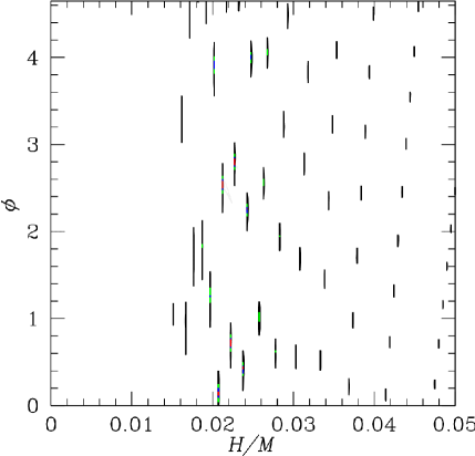
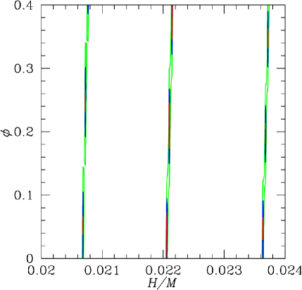
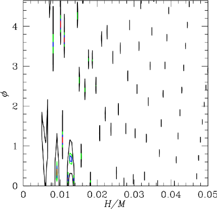
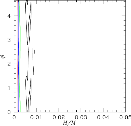
Several conclusions can be drawn from this analysis. First, the projected error ellipses for our hypothetical cosmic-variance limited measurement are extremely small in the $H/M$ plane, indicating a clear ability to detect the trans-Planckian oscillations in the power spectrum. However, because of the presence of a large number of nearly degenerate “islands” in the likelihood function, it will be difficult to pin down the precise values of both the trans-Planckian parameters, especially the phase. This is consistent with the results obtained in previous analyses Elgaroy:2003gq ; Okamoto:2003wk . However, we do note that for the fiducial model chosen, none of the best-fit “islands” is consistent with zero amplitude, $H/M=0$. Therefore, although the values of trans-Planckian parameters are poorly constrained, the case of zero modulation can be ruled out to high significance. Figure 3 shows the shape of the likelihood surface relative to a fiducial model with $H/M=0.01$, and Fig. 4 shows the likelihood relative to the null hypothesis, $H/M=0$, which gives a measure of the size of the upper limit one could place on $H/M$ if no signal were detected. (We emphasize that the $3\sigma$ upper limit of about $H/M<0.0025$ in Fig. 4 does not take into account variations in other cosmological parameters.)

Figure 3: Grid results for a fiducial model with $H/M=0.01$ and $\phi=2.0$, showing the broadening of the degeneracy for smaller amplitude. (Note that the fiducial model is missed due to finite grid size effects.)

Figure 4: Grid results for the null hypothesis, $H/M=0$, estimating an upper limit on $H/M$ if no trans-Planckian signal is detected.

$\begin{array}[]{c@{\hspace{1in}}c}\epsfbox{lam.005.eps}\hfil\hskip 72.26999pt&\epsfbox{lam.005.3d.eps}\\ \epsfbox{lam.01.eps}\hfil\hskip 72.26999pt&\epsfbox{lam.01.3d.eps}\\ \epsfbox{lam.04.eps}\hfil\hskip 72.26999pt&\epsfbox{lam.04.3d.eps}\end{array}$

Figure 5: (Left) The value of $I$ plotted on the $(\lambda,\phi)$ plane, where the purple (gray) lines, white areas and black areas represent $I=1$, $I>1$ and $I<1$ regions respectively. (Right) The 3–d representation of $I$. The underlying “data” has $\phi_{0}=0$ and $\epsilon_{0}=0.15/16=\epsilon$, and the underlying value of $\lambda_{0}$ ranges from (top to bottom) 0.005, 0.01, 0.04 respectively.

$\begin{array}[]{c@{\hspace{1in}}c}\epsfbox{lam.02_fine.eps}\hfil\hskip 72.26999pt\\ \epsfbox{lam.02_fine.3d.eps}\hfil\hskip 72.26999pt\end{array}$

Figure 6: $I$ plotted on the $(\lambda,\phi)$ plane, showing in detail a small region for comparison with Figure 2. The underlying “data” has $\phi_{0}=0.2$, $\epsilon_{0}=0.15/16=\epsilon$, and $\lambda_{0}=0.02$.

Why are these degenerate “islands” present in the parameter space? In order to understand this result in a semi-analytic sense, we consider the effect of the degeneracy on the primordial power spectra. The motivation of the following analysis is that likelihood degeneracies arise from frequency “beating” between underlying modulations in the data and the model. Parameter combinations where “beating” occurs over the largest $k$–ranges give rise to discrete likelihood “islands” or local maxima in the $(H/M)$ vs $\phi$ plane.

Defining the trans-Planckian modification factor multiplying the standard Bunch-Davies power spectrum as

$$\Delta(k,\lambda,\phi,\epsilon)=1+\lambda\left(\frac{k}{k_{\star}}\right)^{-\epsilon}\sin\left[\frac{2}{1-\epsilon}\frac{1}{\lambda}\left(\frac{k}{k_{\star}}\right)^{\epsilon}+\phi\right],$$ (18)

where $\lambda\equiv(H/M)$, we define the parameter $I$ where

$$I=\frac{\int_{0.001}^{0.1}\Delta(k,\lambda,\phi,\epsilon)\Delta(k_{0},\lambda_{0},\phi_{0},\epsilon_{0})dk}{\int_{0.001}^{0.1}\Delta(k_{0},\lambda_{0},\phi_{0},\epsilon_{0})\Delta(k_{0},\lambda_{0},\phi_{0},\epsilon_{0})dk}.$$ (19)

Here, we have performed the integration over the relevant scales for the CMB, $k\sim 0.001{\rm Mpc}^{-1}$ – $0.1{\rm Mpc}^{-1}$. If $I=1$, there will be a near-perfect degeneracy between the parameter sets $(\lambda_{0},\phi_{0},\epsilon_{0})$ and $(\lambda,\phi,\epsilon)$. Assuming that $\epsilon$ can be constrained by detecting tensor modes, a local likelihood maximum is likely to be present at $(\lambda,\phi)$ even though the underlying “data” has $(\lambda_{0},\phi_{0})$.

In the case corresponding to our fiducial models above, $\lambda_{0}=0$, only a simple degeneracy $1/\lambda\propto\pi n-\phi$ exists. In Figures 5, we compute $I$ for several values of non-zero $\lambda=[0.005,0.01,0.04]$. While the results in these figures are in the analytically tractable power-spectrum space, Figure 6 shows a comparison with Figure 2 above, which was calculated the full $C_{\ell}$ formalism. Since convolution with the CMB transfer functions will tend to smear out likelihood degeneracies present in primordial power-spectrum space, we expect the likelihood “islands” to be less prominent in the full $C_{\ell}$ calculation than in the semi-analytic calculation.

These results show that the presence of discrete likelihood maxima in parameter space gives some extra information beyond merely being a numerical headache and a barrier to parameter estimation. Their presence in a parameter estimation analysis is an indication of an underlying modulation in the data, and the appearance of these degeneracies on the $(H/M)$ vs $\phi$ plane in this model is a function of the value of $(H/M)$ of the data. Of course, should such an effect be detected in real data, whether or not such a modulation is due to a primordial effect or some systematic effect in the data, is a question which would need to be investigated thoroughly.

While the grid method is a good tool for exploring the global shape of the likelihood function, it is an oversimplification to vary only two parameters in the fit. Error bars derived from such a two-parameter analysis will be unrealistically optimistic, since a complete analysis must take into account degeneracies between the parameters of interest and a large number of other cosmological parameters. To investigate the effect of including other cosmological parameters in the fit, we apply a Fisher matrix technique in Sec. III.3 and Monte Carlo Markov chain methods in Sec. IV.

III.3 Fisher Matrix

The Fisher matrix technique is a simple and efficient method for estimating the expected measurement errors when marginalizing over a large number of parameters, for which grid methods would be unacceptably time consuming. Measurement uncertainty in cosmological parameters is characterized by the Fisher information matrix $\alpha_{ij}$. (For a review, see Ref. Tegmark:1996bz .) Given a set of parameters $\left\{\lambda_{i}\right\}$, the Fisher matrix is given by

$$\alpha_{ij}=\sum_{l}\sum_{X,Y}{\partial C_{Xl}\over\partial\lambda_{i}}{\rm Cov}^{-1}\left(\hat{C}_{Xl}\hat{C}_{Yl}\right){\partial C_{Yl}\over\partial\lambda_{j}},$$ (20)

where $X,Y=T,E,B,C$ and $\rm{Cov}^{-1}\left(\hat{C}_{Xl}\hat{C}_{Yl}\right)$ is the inverse of the covariance matrix between the estimators $\hat{C}_{Xl}$ of the power spectra. Calculation of the Fisher matrix requires assuming a “true” set of parameters and numerically evaluating the $C_{Xl}$’s and their derivatives relative to that parameter choice. The covariance matrix for the parameters $\left\{\lambda_{i}\right\}$ is just the inverse of the Fisher matrix, $\left(\alpha^{-1}\right)_{ij}$, and the expected error in the parameter $\lambda_{i}$ is of order $\sqrt{\left(\alpha^{-1}\right)_{ii}}$. The full set of parameters $\left\{\lambda_{i}\right\}$ we allow to vary is:

1. tensor/scalar ratio $r$,

2. spectral index $n_{s}$,

3. running $dn_{s}/d\ln k$,

4. normalization $A(k_{*}=0.002\ {\rm Mpc}^{-1})$,

5. baryon density $\Omega_{b},$

6. Hubble constant $h\equiv H_{0}/(100\,{\rm km\,sec^{-1}\,Mpc^{-1}})$,

7. reionization optical depth, $\tau_{\rm ri}$,

8. Cosmological constant density $\Omega_{\Lambda}$,

9. Trans-Planckian amplitude $H/M$,

10. Trans-Planckian phase $\phi$.

The total density is fixed such that the universe is flat, $\Omega_{b}+\Omega_{c}+\Omega_{\Lambda}=1$. Since one needs only to calculate the derivative of the likelihood function with respect to each parameter, Fisher matrix calculations scale linearly with the number of parameters and are therefore very efficient for forecasting errors in fits marginalizing over a large number of parameters. This technique, however, gives no information about the global shape of the likelihood surface. Obviously, since we do not know the values of the trans-Planckian parameters in the real universe, only the size of the errors, not the location of the central value, is significant.

We perform a Fisher matrix analysis for two different forecast data sets: first, in order to understand the best-case scenario, we consider a measurement for which the errors are limited by cosmic variance to $\ell=1500$, similar to that assumed for the grid method in Sec. III.2. Second, we consider the more immediately realistic case of a measurement with error bars similar to those projected for the Planck Surveyor satellite, for which we assume a two-channel experiment measuring both temperature and polarization. The 143 GHz channel is assumed to have an $8$-arcminute beam and a pixel sensitivity of $\sigma_{\rm pix}=5.5\ {\rm\mu K}$, and the 217 GHz channel is assumed to have an $5.5$-arcminute beam and a pixel sensitivity of $\sigma_{\rm pix}=11.7\ {\rm\mu K}$.

We are especially interested in the degeneracy between trans-Planckian modulations and the other parameters determining the shape of the primordial power spectrum, $n_{s}$ and $dn_{s}/d\ln k$. This degeneracy is highly dependent on the value of $r$ in the underlying fiducial model we choose, because for small $r$, the trans-Planckian modulation becomes very long-wavelength and thus mimics a change in the spectral index $n_{s}$ or running $dn_{s}/d\ln k$ (Fig. 7). (For the case $r=0$, the “modulation” loses all scale-dependence and simply affects the normalization. The value of $H/M$ thus decouples from the other parameters determining the shape of the power spectrum, and the degeneracy vanishes in this limit.)

$\begin{array}[]{c@{\hspace{1in}}c}\epsfbox{r0.02_apower.eps}\hfil\hskip 72.26999pt&\epsfbox{r0.05_apower.eps}\\ \epsfbox{r0.1_apower.eps}\hfil\hskip 72.26999pt&\epsfbox{r0.2_apower.eps}\\ \end{array}$

Figure 7: Modulation of the power spectrum for various choices of $r$: $r=0.02$ (top left), $r=0.05$ (top right), $r=0.1$, (bottom left), and $r=0.2$ (bottom right). In all cases the solid (cyan) line is the unmodulated spectrum, and the points represent the modulated power spectrum as sampled by CMBFAST.

We therefore plot error ellipses in the $n_{s}$ - $H/M$ plane and the $dn_{s}/d\ln k$ - $H/M$ plane for various choices for $r$ running from $r=0.02$ to $0.2$. The fiducial model assumed in all cases has $H/M=0.01$ and phase $\phi=0$. Other parameters are identical to those used for the grid calculation in Sec. III.2. Figure 8 shows the $n_{s}$ - $H/M$ plane for the case of the cosmic-variance limited measurement, and Fig. 10 shows the $dn_{s}/d\ln k$ - $H/M$ plane. In this case, the measurement is sufficiently accurate that the degeneracy between the power spectrum parameters $n_{s}$, $dn_{s}/d\ln k$ and the trans-Planckian amplitude $H/M$ is negligible, although the ability to constrain $H/M$ is significantly degraded for small values of $r$. These error estimates can be directly compared with those generated by a full Markov Chain Monte Carlo analysis with similar parameters, (Figs. 12 and 13), and are in good agreement.

Figure 8: $2\sigma$ error ellipses in the $n_{s}$ - $H/M$ plane, calculated by Fisher matrix, assuming a fiducial model with $n_{s}=0.93$ and $H/M$ = 0.01 and a cosmic-variance limited measurement to $\ell=1500$. The different ellipses show the effect of changing the choice of tensor/scalar ratio $r$ in the fiducial model: larger values of $r$ make it easier to distinguish the trans-Planckian modulation. The top panel shows ellipses for $r=0.02$ (black, outer), $r=0.05$ (blue, next in), $r=0.1$ (green, second smallest), and $r=0.2$ (red, inner). The bottom panel shows the same figure zoomed in to show the three inner ellipses. (Negative values for $H/M$ are nonphysical, and are included to show the full error ellipse.)

Figure 9: $2\sigma$ error ellipses in the $n_{s}$ - $H/M$ plane, calculated by Fisher matrix, assuming a fiducial model with $n_{s}=0.93$ and $H/M$ = 0.01 and an observation with the projected sensitivity of the Planck Surveyor satellite. The different ellipses show the effect of changing the choice of tensor/scalar ratio $r$ in the fiducial model: larger values of $r$ make it easier to distinguish the trans-Planckian modulation. The top panel shows ellipses for $r=0.02$ (black, outer), $r=0.05$ (blue, next in), $r=0.1$ (green, second smallest), and $r=0.2$ (red, inner). The bottom panel shows the same figure zoomed in to show the three inner ellipses.

Figure 10: $2\sigma$ error ellipses in the $dn_{s}/d\ln k$ - $H/M$ plane, calculated by Fisher matrix, assuming a fiducial model with $n_{s}=0.93$ and $H/M$ = 0.01 and a cosmic-variance limited observation. The different ellipses show the effect of changing the choice of tensor/scalar ratio $r$ in the fiducial model: larger values of $r$ make it easier to distinguish the trans-Planckian modulation. The top panel shows ellipses for $r=0.02$ (black, outer), $r=0.05$ (blue, next in), and $r=0.1$ (green, smallest). The bottom panel shows the same figure zoomed in to show the three inner ellipses.

Figure 11: $2\sigma$ error ellipses in the $dn_{s}/d\ln k$ - $H/M$ plane, calculated by Fisher matrix, assuming a fiducial model with $n_{s}=0.93$ and $H/M$ = 0.01 and an observation with the projected sensitivity of the Planck Surveyor satellite. The different ellipses show the effect of changing the choice of tensor/scalar ratio $r$ in the fiducial model: larger values of $r$ make it easier to distinguish the trans-Planckian modulation. The top panel shows ellipses for $r=0.02$ (black, outer), $r=0.05$ (blue, next in), $r=0.1$ (green, second smallest), and $r=0.2$ (red, inner). The bottom panel shows the same figure zoomed in to show the three inner ellipses.

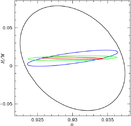
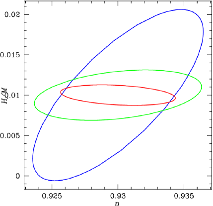
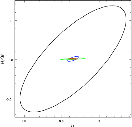
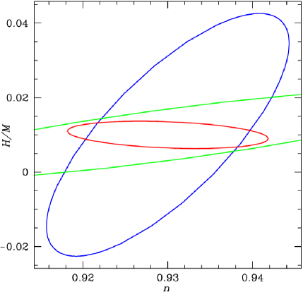
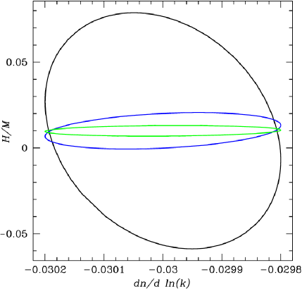
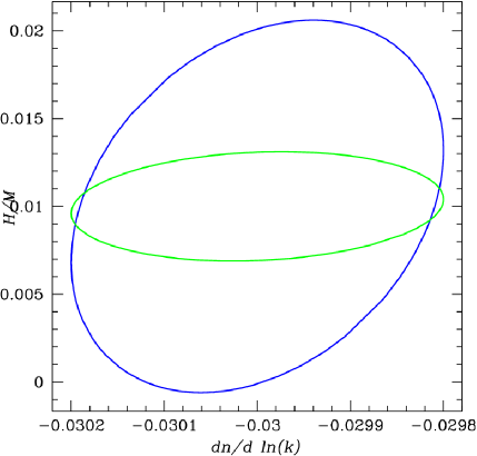
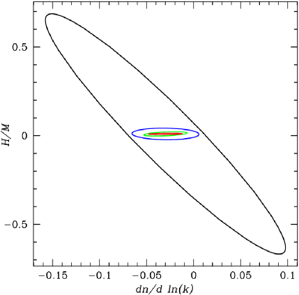
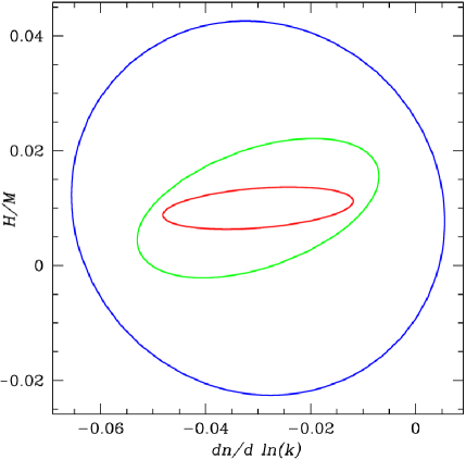
This situation is very different for the case of Planck Surveyor, shown in Figs. 9 and 11 for the $n_{s}$ - $H/M$ and $dn_{s}/d\ln k$ - $H/M$ planes, respectively. We see that in this case, the inclusion of a trans-Planckian modulation in the parameter set strongly degrades the ability to measure the power spectrum parameters. This degeneracy is lifted if the tensor/scalar ratio is large enough, effectively disappearing altogether for a tensor/scalar ratio of order $r\sim 0.1$.

Finally, as expected, the measurement uncertainties on the trans-Planckian parameters increase significantly when a full set of other cosmological parameters is taken into account. The Fisher matrix analysis is in good agreement with the full Markov Chain Monte Carlo analysis discussed in Sec. IV, indicating that a trans-Planckian modulation of order $H/M=0.01$ is only detectable at the $2\sigma$ level in the most optimistic case of a very large tensor/scalar ratio $r\sim 0.1$. In the next section we discuss the MCMC analysis in detail and derive the error ellipses relative to a fiducial model with $H/M=0$, testing our ability to distinguish a signal from the null hypothesis. This analysis (which includes a longer lever arm of $\ell=2000$), indicates that a cosmic-variance limited measurement can place a $2\sigma$ upper limit on trans-Planckian fluctuations of around $H/M=0.004$ for the case with a large tensor/scalar ratio ($r=0.15$), and $H/M=0.03$ for the case with an undetectably small tensor/scalar ratio.

IV Markov Chains

IV.1 Introduction

In this section, we use a Markov Chain Monte Carlo (MCMC) technique to evaluate the likelihood function of model parameters. This approach, proposed by Christensen:2000ji in the context of cosmological parameter estimation, has become the standard tool for such analyses (e.g. Christensen:2001gj, ; Knox:2001fz, ; Lewis:2002ah, ; Kosowsky:2002zt, ; Verde:2003ey, ). MCMC is a method to simulate posterior distributions. In particular, we simulate observations from the posterior distribution ${\cal P}({\bf\alpha}|x)$, of a set of parameters ${\bf\alpha}$ given event $x$, obtained via Bayes’ Theorem,

$${\cal P}(\alpha|x)=\frac{{\cal P}(x|\alpha){\cal P}(\alpha)}{\int{\cal P}(x|\alpha){\cal P}(\alpha)d\alpha},$$ (21)

where ${\cal P}(x|\alpha)$ is the likelihood of event $x$ given the model parameters $\alpha$ and ${\cal P}(\alpha)$ is the prior probability density. The MCMC generates random draws (i.e. simulations) from the posterior distribution that are a “fair” sample of the likelihood surface. From this sample, we can estimate all of the quantities of interest about the posterior distribution (mean, variance, confidence levels). The MCMC method scales approximately linearly with the number of parameters, thus allowing us to perform a likelihood analysis in a reasonable amount of time.

A properly derived and implemented MCMC draws from the joint posterior density ${\cal P}(\alpha|x)$ once it has converged to the stationary distribution. For our application, $\alpha$ denotes a set of 10 parameters. The set is almost the same as used for the Fisher matrix calculation. We have 4 “late-time” parameters: the physical energy density in baryons $\Omega_{b}h^{2}$, the total physical energy density in matter $\Omega_{m}h^{2}$, the optical depth to reionization $\tau_{\rm ri}$, the Hubble constant in units of $100$ km s^-1 Mpc – $h$. There are 6 “primordial parameters”: the tensor-to-scalar ratio $r$, the spectral slope $n_{s}$, the running of the spectral slope $dn_{s}/d\ln k$, the power spectrum amplitude $A$, and the parameters of the trans-Planckian model defined above, $H/M$ and $\phi$. Event $x$ will be the set of observed $\widehat{\cal C}_{\ell}$. The priors on the model are that the universe is flat, so that $\Omega_{m}+\Omega_{\Lambda}=1$, and the dark energy is a cosmological constant with equation of state $p=-\rho$. The definitions used for the unmodified primordial power spectra of the scalar and tensor perturbations $\Delta^{2}_{\cal R,BD}(k)\equiv k^{3}/(2\pi^{2})\langle\left|{\cal R}_{\mathbf{k}}\right|^{2}\rangle\propto k^{n_{s}-1}$ and $\Delta^{2}_{h,BD}(k)\equiv 2k^{3}/(2\pi^{2})\langle\left|h_{+{\mathbf{k}}}\right|^{2}+\left|h_{\times{\mathbf{k}}}\right|^{2}\rangle\propto k^{n_{t}}$ are given in Section II.

IV.2 Methodology

The experiment in the case study is considered to measure ${TT,TE,EE,BB}$ power spectra to $\ell=2000$; beyond this, the systematic errors in removing the contamination from secondary CMB anisotropies are likely to be non-negligible. We include the effect of weak lensing on all power spectra, since this is the “theoretical limit” in the accuracy of the measurement - weak lensing aliases power between multipoles and tends to smooth out small-scale oscillations in the data. Therefore, any of the further uncertainties that must be accounted for in a practical CMB experiment, such as foreground removal, partial sky coverage etc, will degrade the constraints obtainable on the trans-Planckian parameters relative to those found in this study.

For the simulated “data”, we consider two cases: one with significant primordial tensor modes (denoted Case H), and one with an undetectably small contribution of primordial tensors (denoted case L). Case H is a mass-term inflation model with tensor-to-scalar ratio $r=0.15$ which is consistent with WMAP data at the $1\sigma$ level. Case L is simply the WMAP LCDM concordance model with $r=0.00013$ (quadrupole ratio $C_{2}^{T}/C_{2}^{S}\sim 6\times 10^{-5}$).

The objective of this study is to see how far from the null case the trans-Planckian parameters must be before they are distinguished from the null model by at least $2\sigma$. Consequently, these fiducial models do not contain any trans-Planckian oscillations. Our fiducial models also do not contain any running of the primordial scalar spectral index; however, the effect of this parameter would be degenerate with a very long wavelength trans-Planckian modulation. Hence we marginalize over this parameter in our analysis.

In the practical implementation of the MCMC, we ran 16 chains for Case H and 32 chains for Case L, each started at random $3\sigma$ steps away from the fiducial model. By making use of preliminary test chains, the proposal distribution was calibrated using the covariance between the parameters in order to minimize correlations; the chains were configured to step in the principal directions of the parameter covariance matrix optimal $\sim 24$% acceptance rates for case H; for case L, only a few % acceptance rates were achieved even after several recalibrations of the proposal matrix, indicating the complexity of the likelihood surface. The chains were run on a high-performance 64-bit Opteron Beowulf cluster, and 300,000 and 500,000 total models were computed for Case H and Case L, respectively. The presence of “islands” in the likelihood space meant that the chains converged relatively slowly, compared to what is typical for a fit to CMB observations when the trans-Planckian terms are absent. In fact, we stopped the chains for Case L slightly short of full convergence, but long after the predicted parameter regions had stabilized.

IV.3 The Shape of the Likelihood Surface

Tables 1 and 2 show the fiducial models and recovered marginalized 1–d 68% probability parameter constraints on the ten model parameters for Case H and Case L, respectively. Figures 12 and 13 show the marginalized 2–d joint 68% and 95% confidence regions for pairs of the six “primordial” parameters for the same models. In Case H, which has potentially observable primordial tensor modes, a deviation of $H/M$ from null is detectable at greater than $2\sigma$ level if $(H/M)>0.004$ in an ideal experiment, which renders $H/M\sim 0.01$ potentially detectable in a real-world experiment. In Case L, which has unobservably small primordial tensor modes, one requires $(H/M)>0.03$ in order to be detectable at greater than the $2\sigma$ level in an ideal experiment, rendering such a detection implausible in the real world. Ref. Okamoto:2003wk discussed a degeneracy between $\epsilon$ and $(H/M)$ which appears to be essentially eliminated in our model due to the extra constraint on $\epsilon$ from tensor modes.

Figure 12: Case H: A fiducial model with $r=0.15$ and no trans-Planckian modulations. The 2-d joint 68% (dark) and 95% (light) confidence regions for pairs of parameters in the set {$r$, $n_{s}$, $dn_{s}/d\ln k$, $A$, $H/M$, $\phi$} obtained via MCMC methods. In the case of each parameter pair, all the other eight parameters in the model have been marginalized over. The discrete “blobs” in the ($n_{s}$, $dn_{s}/d\ln k$) plane are not physical but a graphical effect arising as consequence of binning of a narrow likelihood degeneracy.

Figure 13: Case L: A fiducial model with $r=0.00013$ and no trans-Planckian modulations. The 2-d joint 68% (dark) and 95% (light) confidence regions for pairs of parameters in the set {$r$, $n_{s}$, $dn_{s}/d\ln k$, $A$, $H/M$, $\phi$} obtained via MCMC methods. In the case of each parameter pair, all the other eight parameters in the model have been marginalized over. The discrete “blobs” in the ($n_{s}$, $dn_{s}/d\ln k$) plane are not physical but a graphical effect arising as consequence of binning of a narrow likelihood degeneracy.

Table 1: Case H: A fiducial model with $r=0.15$ and no trans-Planckian modulations. The input model, recovered mean parameters and the 68% probability level of the 1–d marginalized likelihood. The derived parameter $\sigma_{8}$ (the linear theory prediction for the amplitude of fluctuations within 8 Mpc/h spheres) is given in the last row.

Parameter	Input	Recovered
$\Omega_{b}h^{2}$	$0.02273$	$0.02273\pm 0.00006$
$\Omega_{m}$	$0.3097$	$0.3096\pm 0.0016$
$h$	$0.684$	$0.684\pm 0.001$
$\tau_{\rm ri}$	$0.112$	$0.112\pm 0.002$
$n_{s}(k_{\star}=0.002\ {\rm Mpc}^{-1})$	$0.962$	$0.964\pm 0.013$
$dn_{s}/d\ln k$	$0$	$0.000\pm 0.004$
$A(k_{\star}=0.002\ {\rm Mpc}^{-1})$	$0.879$	$0.878\pm 0.016$
$r(k_{\star}=0.002\ {\rm Mpc}^{-1})$	$0.150$	$0.150\pm 0.004$
$H/M$	$0$	$0.002\pm 0.002$
$\phi$	$0$	(degeneracy; mean 0.02)
$\sigma_{8}$		$0.871\pm 0.001$

Table 2: Case L: A fiducial model with $r=0.00013$ and no trans-Planckian modulations. The input model, recovered mean parameters and the 68% probability level of the 1–d marginalized likelihood. The derived parameter $\sigma_{8}$ (the linear theory prediction for the amplitude of fluctuations within 8 Mpc/h spheres) is given in the last row.

Parameter	Input	Recovered
$\Omega_{b}h^{2}$	$0.02380$	$0.02379\pm 00006$
$\Omega_{m}$	$0.2943$	0.$2945\pm 0.0016$
$h$	$0.700$	$0.700\pm 0.001$
$\tau_{\rm ri}$	$0.166$	$0.166\pm 0.002$
$n_{s}(k_{\star}=0.002\ {\rm Mpc}^{-1})$	$0.994$	$0.993\pm 0.010$
$dn_{s}/d\ln k$	$0$	$0.000\pm 0.003$
$A(k_{\star}=0.002\ {\rm Mpc}^{-1})$	$0.900$	$0.900\pm 0.020$
$r(k_{\star}=0.002\ {\rm Mpc}^{-1})$	$0.00013$	$0.00014\pm 0.00004$
$H/M$	$0$	$0.02\pm 0.02$
$\phi$	$0$	(degeneracy; mean 0.05)
$\sigma_{8}$		$0.927\pm 0.001$

The key observations to be drawn from these results are:

1. The constraint on $H/M$ differs by an order of magnitude between Case H and Case L. This reinforces the point made above that if our Universe happens to be in a favorable part of the parameter space where the energy scale of inflation is high enough to produce an observable amplitude of primordial tensor modes, then one has a significantly improved chance of detecting any trans-Planckian modifications to the spectrum whose properties are similar to those of the case tested here.

2. The cosmological parameters are constrained at the $\sim 1\%$ level except for the scalar spectral index and the amplitude of fluctuations at $k=0.002\ {\rm Mpc}^{-1}$, which are only constrained at the $\sim 10\%$ level. Therefore, another cosmological data-set that aids in constraining these parameters (for example, the proposed SKA survey, Rawlings:2004wk ) will minimize the degeneracies with these parameters shown in Figs.12 and 13 and improve parameter constraints further Hannestad:2004ts .

V Conclusion

We believe that this analysis is the most thorough investigation of the detectability of a trans-Planckian modulation to the primordial power spectrum that has been performed to date. We consider three complementary approaches – a simple grid search, a Fisher matrix evaluation of the likely error ellipses, and a Monte Carlo Markov Chain fit to a simulated CMB spectrum, and find that they are all in broad agreement. Moreover, we also explain the “islands” seen in the likelihood space in previous papers on this topic Elgaroy:2003gq ; Okamoto:2003wk , and show that their distribution and properties can be understood and reproduced via a simple analytic argument.

The approach we have taken here is analyze a specific ansatz for introducing a minimum length into the calculation of the perturbation spectrum in a general model of slow-roll inflation Easther:2002xe . We do not claim that this model is a correct description of the trans-Planckian contribution to the perturbation spectrum, but intend it as a case study of what might be possible if one has a specific and well-motivated correction to the spectrum that leads to a $k$ dependent modulation. There is considerable theoretical uncertainty surrounding this point, and it is entirely possible that a future rigorous calculation of the perturbation spectrum within string theory or some other model of ultra high energy physics will predict that there is no modulation to be observed, and the bound calculated here will not apply.

We believe that the constraint obtained here is applicable to a general class of modulated spectra. In practice, one can imagine adding an arbitrary modulation to the primordial spectrum, as considered by Okamoto and Lim Okamoto:2003wk , in which case one has parameters which describe the amplitude, wavelength, and phase of the modulation as a function of $k$. In our model there are only two free parameters – the phase of the modulation, and $H/M$ which determines the amplitude. The phase will always be arbitrary in the absence of detailed theory that matches specific scales in the present universe to those during inflation, which would require a full understanding of the post-inflationary expansion history and the physics of reheating, while the amplitude is directly related to the scale of new physics, which is what we are trying to measure. However, the wavelength of the oscillation turns out to be given in terms of the slow-roll parameter $\epsilon$, which is itself directly related to the tensor/scalar ratio $r$. This dependence is easy to understand, since the form of the modulation is not determined by the (fixed) boundary condition, but by the slow variation in the horizon size $H^{-1}$ with time. The precise functional form of the connection between $\epsilon$ and the modulated spectrum may vary in other specific models. However, it is very likely that the modulation can always be expressed in terms of $H/M$ and the scale dependence of $H$ – or thus $\epsilon$, and perhaps the higher order slow-roll parameters, which are also reachable through their contribution to the scalar spectral index. Consequently, we believe that the results we have seen here will generalize to other modulated spectra, even though we have reduced the number of trans-Planckian parameters relative to those considered by Okamoto and Lim.

The second general conclusion we draw is that the detectability of any modulated spectrum depends on the value of $H$. Since the wavelength of the modulation depends on $\epsilon$, detecting the primordial tensors provides an orthogonal constraint on the value of this parameter, and thus constrains the trans-Planckian corrections. Since $H$ fixes the energy scale at which inflation occurs, it is arguably the single most interesting cosmological parameter that is not currently fixed by observations. The analysis here simply adds to the importance of this parameter, since we have shown that measuring $H$ will put tighter bounds on any trans-Planckian corrections to the spectrum.

Since the theoretical uncertainty about the form and existence of these corrections is yet to be resolved, we cannot advocate mounting an observational campaign solely to look for this kind of signal. However, there is already good and sufficient reason to make an all out effort to measure $H$ during inflation, via high precision measurements of the CMB and particularly its polarization. We believe that mission planners will want to be aware of the possibility that precision CMB measurements may potentially probe physics at the string scale, since this will not add to the cost of any mission but represents an exciting and additional use of the data they can be expected to return.

In quantitative terms, we see that the with a large ($r\sim 0.15$) value of the tensor to scalar ratio, a “perfect” map of the primordial temperature and polarization anisotropies to the CMB could rule out a trans-Planckian modulation to the spectrum at the $2\sigma$ level for $H/M\sim 0.004$. This is roughly the same as the result reported by Okamoto and Lim. We vary a larger set of cosmological parameters than they do, which reduces the level of precision we can hope for. However by adding the tensor contribution to the analysis and removing a free parameter from the specification of modulation we can tighten the bound. Like Okamoto and Lim, we consider a perfect measurement of the CMB and any real experiment will be contaminated by imperfectly removed foregrounds. Consequently, we believe that a value of $H/M$ on the order of 0.01 represents a reasonable lower bound on what can be detected in practice, provided the amplitude of the tensor contribution is significant. On the other hand, adding other orthogonal datasets, such as a measurement of $h$ and the late time expansion history of the universe from a SNAP-like mission, or constraints on the primordial spectrum from future large scale structure surveys will further constrain the error ellipses relative to those which can be achieved via the CMB alone.

At this point, the theoretical uncertainty surrounding this calculation makes it unwise to push this analysis significantly further. However, we believe that considerable progress has been made in understanding the physical issues surrounding the trans-Planckian corrections to the primordial spectrum over the last few years. Consequently, it is not excessively optimistic to hope that the remaining issues can be resolved on a shorter timescale than it will take to perform a measurement of the CMB that even approaches the precision we have assumed in our analysis. In this light, we are particularly interested in the effective field theory approach taken in Schalm:2004qk , and extended in the more recent preprint Greene:2004np . In this case, the operators which can contribute to a modification to the spectrum can be cataloged within effective field theory. From the observational perspective, an analogous calculation to the one presented here will constrain the values of the prefactors in front of these operators, and we intend to pursue this in future work.

References

- (1) R. H. Brandenberger, arXiv:hep-ph/9910410.
- (2) A. Kempf, Phys. Rev. D 63, 083514 (2001) [arXiv:astro-ph/0009209].
- (3) J. Martin and R. H. Brandenberger, Phys. Rev. D 63, 123501 (2001) [arXiv:hep-th/0005209].
- (4) R. H. Brandenberger and J. Martin, Mod. Phys. Lett. A 16, 999 (2001) [arXiv:astro-ph/0005432].
- (5) J. C. Niemeyer, Phys. Rev. D 63, 123502 (2001) [arXiv:astro-ph/0005533].
- (6) R. Easther, B. R. Greene, W. H. Kinney and G. Shiu, Phys. Rev. D 64, 103502 (2001) [arXiv:hep-th/0104102].
- (7) R. Easther, B. R. Greene, W. H. Kinney and G. Shiu, Phys. Rev. D 67, 063508 (2003) [arXiv:hep-th/0110226].
- (8) J. C. Niemeyer and R. Parentani, Phys. Rev. D 64, 101301 (2001) [arXiv:astro-ph/0101451].0
- (9) A. Kempf and J. C. Niemeyer, Phys. Rev. D 64, 103501 (2001) [arXiv:astro-ph/0103225].
- (10) U. H. Danielsson, Phys. Rev. D 66, 023511 (2002) [arXiv:hep-th/0203198].
- (11) R. Easther, B. R. Greene, W. H. Kinney and G. Shiu, Phys. Rev. D 66, 023518 (2002) [arXiv:hep-th/0204129].
- (12) N. Kaloper, M. Kleban, A. E. Lawrence and S. Shenker, Phys. Rev. D 66, 123510 (2002) [arXiv:hep-th/0201158].
- (13) R. H. Brandenberger and J. Martin, Int. J. Mod. Phys. A 17, 3663 (2002) [arXiv:hep-th/0202142].
- (14) J. Martin and R. Brandenberger, Phys. Rev. D 68, 063513 (2003) [arXiv:hep-th/0305161].
- (15) K. Schalm, G. Shiu and J. P. van der Schaar, arXiv:hep-th/0401164.
- (16) S. Shankaranarayanan and L. Sriramkumar, arXiv:hep-th/0403236.
- (17) A. Liddle and D. Lyth Cosmological Inflation and Large Scale Structure, Cambridge UP (2000)
- (18) V. S. Kaplunovsky, Nucl. Phys. B 307, 145 (1988) [Erratum-ibid. B 382, 436 (1992)] [arXiv:hep-th/9205068].
- (19) N. Arkani-Hamed, S. Dimopoulos and G. R. Dvali, Phys. Lett. B 429, 263 (1998) [arXiv:hep-ph/9803315].
- (20) I. Antoniadis, N. Arkani-Hamed, S. Dimopoulos and G. R. Dvali, Phys. Lett. B 436, 257 (1998) [arXiv:hep-ph/9804398].
- (21) V. Bozza, M. Giovannini and G. Veneziano, JCAP 0305, 001 (2003) [arXiv:hep-th/0302184].
- (22) D. H. Lyth, Phys. Rev. Lett. 78, 1861 (1997) [arXiv:hep-ph/9606387].
- (23) L. Knox and Y. S. Song, Phys. Rev. Lett. 89, 011303 (2002) [arXiv:astro-ph/0202286].
- (24) M. Kesden, A. Cooray and M. Kamionkowski, Phys. Rev. Lett. 89, 011304 (2002) [arXiv:astro-ph/0202434].
- (25) U. Seljak and C. M. Hirata, Phys. Rev. D 69, 043005 (2004) [arXiv:astro-ph/0310163].
- (26) J. Khoury, B. A. Ovrut, P. J. Steinhardt and N. Turok, Phys. Rev. D 64, 123522 (2001) [arXiv:hep-th/0103239].
- (27) M. Gasperini and G. Veneziano, Astropart. Phys. 1, 317 (1993) [arXiv:hep-th/9211021].
- (28) J. E. Lidsey, D. Wands and E. J. Copeland, Phys. Rept. 337, 343 (2000) [arXiv:hep-th/9909061].
- (29) J. E. Lidsey, A. R. Liddle, E. W. Kolb, E. J. Copeland, T. Barreiro and M. Abney, Rev. Mod. Phys. 69, 373 (1997) [arXiv:astro-ph/9508078].
- (30) R. Easther, arXiv:hep-th/0407042.
- (31) C. P. Burgess, J. M. Cline, F. Lemieux and R. Holman, JHEP 0302, 048 (2003) [arXiv:hep-th/0210233].
- (32) L. Sriramkumar and T. Padmanabhan, arXiv:gr-qc/0408034.
- (33) L. Bergstrom and U. H. Danielsson, JHEP 0212, 038 (2002) [arXiv:hep-th/0211006].
- (34) O. Elgaroy and S. Hannestad, Phys. Rev. D 68, 123513 (2003) [arXiv:astro-ph/0307011].
- (35) T. Okamoto and E. A. Lim, [arXiv:astro-ph/0312284].
- (36) J. Martin and C. Ringeval, Phys. Rev. D 69, 083515 (2004) [arXiv:astro-ph/0310382].
- (37) J. Martin and C. Ringeval, Phys. Rev. D 69, 127303 (2004) [arXiv:astro-ph/0402609].
- (38) J. Martin and C. Ringeval, arXiv:hep-ph/0405249.
- (39) L. Verde et al., Astrophys. J. Suppl. 148, 195 (2003) [arXiv:astro-ph/0302218].
- (40) W. H. Kinney, Phys. Rev. D 56, 2002 (1997) [arXiv:hep-ph/9702427].
- (41) A. Ashoorioon, A. Kempf and R. B. Mann, arXiv:astro-ph/0410139.
- (42) C. Armendariz-Picon and E. A. Lim, JCAP 0312, 006 (2003) [arXiv:hep-th/0303103].
- (43) U. Seljak and M. Zaldarriaga, Astrophys. J. 469, 437 (1996) [arXiv:astro-ph/9603033].
- (44) M. Tegmark, A. Taylor and A. Heavens, Astrophys. J. 480, 22 (1997) [arXiv:astro-ph/9603021].
- (45) N. Christensen and R. Meyer, arXiv:astro-ph/0006401.
- (46) N. Christensen, R. Meyer, L. Knox and B. Luey, Class. Quant. Grav. 18, 2677 (2001) [arXiv:astro-ph/0103134].
- (47) A. Kosowsky, M. Milosavljevic and R. Jimenez, Phys. Rev. D 66, 063007 (2002) [arXiv:astro-ph/0206014].
- (48) A. Lewis and S. Bridle, Phys. Rev. D 66, 103511 (2002) [arXiv:astro-ph/0205436].
- (49) L. Knox, N. Christensen and C. Skordis, arXiv:astro-ph/0109232.
- (50) S. Rawlings, F. B. Abdalla, S. L. Bridle, C. A. Blake, C. M. Baugh, L. J. Greenhill and J. M. van der Hulst, arXiv:astro-ph/0409479.
- (51) S. Hannestad and L. Mersini-Houghton, arXiv:hep-ph/0405218.
- (52) B. R. Greene, K. Schalm, G. Shiu and J. P. van der Schaar, arXiv:hep-th/0411217.