A Concordance Model of The Lyman-Alpha Forest at z = 1.95

Abstract

We present 40 fully hydrodynamical numerical simulations of the intergalactic gas that gives rise to the Ly$\alpha$ forest. The simulation code, input and output files are available at http://www.cosmos.ucsd.edu/g̃so/index.html. For each simulation we predict the observable properties of the H I absorption in QSO spectra. We then find the sets of cosmological and astrophysical parameters that match the QSO spectra. We present our results as scaling relationships between input and output parameters. The input parameters include the main cosmological parameters $\Omega_{b}$, $\Omega_{m}$, $\Omega_{\Lambda}$, $H_{0}$ and $\sigma_{8}$; and two astrophysical parameters $\gamma_{912}$ and $X_{228}$. The parameter $\gamma_{912}$ controls the rate of ionization of H I, He I and He II and is equivalent to the intensity of the UV background. The second parameter $X_{228}$ controls the rate of heating from the photoionization of He II and can be related to the shape of the UVB at $\lambda<228$ Å. We show how these input parameters; especially $\sigma_{8}$, $\gamma_{912}$ and $X_{228}$; effect the output parameters that we measure in simulated spectra. These parameters are the mean flux $\bar{F}$, a measure of the most common Ly$\alpha$ line width ($b$-value) $b_{\sigma}$, and the 1D power spectrum of the flux on scales from 0.01 – 0.1 s/km. We compare the simulation output to data from Kim et al. (2004) and Tytler et al. (2004) and we give a new measurement of the flux power from HIRES and UVES spectra for the low density IGM alone at $z=1.95$.

We find that simulations with a wide variety of $\sigma_{8}$ values, from at least 0.8 – 1.1, can fit the small scale flux power and $b$-values when we adjust $X_{228}$ to compensate for the $\sigma_{8}$ change. We can also use $\gamma_{912}$ to adjust the H I ionization rate to simultaneously match the mean flux. When we examine only the mean flux, $b$-values and small scale flux power we can not readily break the strong degeneracy between $\sigma_{8}$ and $X_{228}$.

We can break the degeneracy using large scale flux power or other data to fix $\sigma_{8}$. When we pick a specific $\sigma_{8}$ value the simulations give $X_{228}$ and hence the IGM temperature that we need to match the observed small scale flux power and $b$-values. We can then also find the $\gamma_{912}$ required to match the mean flux for that combination of $\sigma_{8}$ and $X_{228}$. We derive scaling relations that give the output parameter values expected for a variety of input parameters. We predict the line width parameter $b_{\sigma}$ with an error of 1.4% and the mean amount of H I absorption to 2%, equivalent to a 0.27% error on $\bar{F}$ ar $z=1.95$. These errors are four times smaller than those on the best current measurement. We can readily calculate the sets of input parameters that give outputs that match the data. For $\sigma_{8}$$=0.9$, with $\Omega_{b}$$=0.044$, $\Omega_{m}$$=0.27$, $\Omega_{\Lambda}$$=0.73$, $h=0.71$ and $n=1.0$ we find $X_{228}$$=1.26$ and $\gamma_{912}$$=1.00$, equivalent to $\Gamma_{912}=1.33\times 10^{-12}$ ionizations per H I atom per second. If we run an optically thin simulation with these input parameter values in a box size of 76.8 Mpc comoving with cells of 18.75 kpc comoving we expect that the simulated spectra will match Ly$\alpha$ forest data at $z=1.95$. The rates predicted by Madau et al. (1999) correspond to $\gamma_{912}$$=1$ and $X_{228}$$=1$. We are in accord for $\gamma_{912}$ while the larger $X_{228}$ is reasonable to correct for the opacity that is missing from the optically thin simulations. To match data for smaller $\sigma_{8}$, structure is more extended and we need a smaller $X_{228}$ corresponding to a cooler IGM. We also need a larger $\gamma_{912}$ to stop the neutral fraction from increasing at the lower temperatures.

1 Introduction

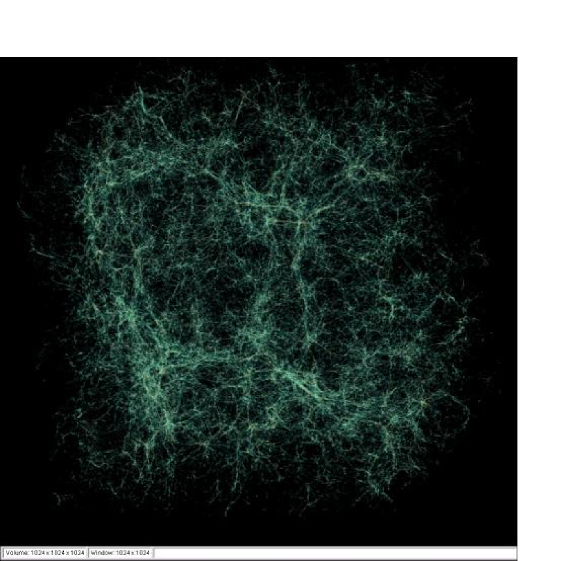
Figure 1: Volumetric rendering of the log baryon density from simulation A at $z=2.0$.

Hydrodynamic cosmological simulations (Cen et al., 1994; Zhang et al., 1995; Hernquist et al., 1996; Miralda-Escude et al., 1996; Zhang et al., 1997, 1998; Wadsley & Bond, 1997; Theuns et al., 1998) have revolutionized our understanding of Lyman alpha forest absorption lines seen in the spectra of high redshift QSOs. Based on the impressive agreement between simulations and observations on a variety of HI absorption line statistics (see Rauch (1998) for a review) it is now widely accepted that the HI Ly$\alpha$ absorption is caused by mildly overdense, highly photoionized intergalactic gas that closely traces the dark matter distribution in CDM models of structure formation. According to these simulations, on scales of a Mpc or more, the dark matter and baryons trace out a network of sheets and filaments (Fig. 1) referred to as the cosmic web arising from the growth of primordial matter fluctuations (Bond et al., 1996).

The intimate physical connection between absorption and dark matter density has stimulated many researchers (Croft et al., 1998, 2002; McDonald et al., 2000; McDonald, 2003; McDonald et al., 2004a; Zaldarriaga et al., 2001; Mandelbaum et al., 2003; Seljak et al., 2003, 2004; Viel et al., 2004a) to explore the possibility of using observations of the Ly$\alpha$ forest as a cosmological probe of the z=2-4 universe in much the same way as observations of CMB anisotropies have been used to probe the z=1300 universe (Spergel et al., 2003). The forest probes the primordial power spectrum on scales an order of magnitude smaller than the highest resolution CMB experiments. The function that assumes the role of the CMB angular power spectrum is the flux power spectrum. This is essentially the Fourier transform of transmitted flux spectrum averaged over many lines of sight (we will define it more precisely below). The current state-of-the-art is the work of (Seljak et al., 2004) who have measured the amplitude and shape of the matter power spectrum by combining SDSS and WMAP results. They find consistency with the best fit WMAP LCDM model with $\mbox{$\sigma_{8}$}=0.90\pm 0.03$ and a primordial slope $n=0.98\pm 0.02$.

Somewhat decoupled from this effort, other researchers have used observations of the Ly$\alpha$ forest and hydrodynamic simulations to probe the thermal and ionization state of the IGM at high redshift (Rauch et al., 1997; Schaye et al., 1999, 2000; Bryan & Machacek, 2000; Theuns et al., 2000; Tytler et al., 2004; Bolton et al., 2004). Simulations and analytic studies have shown that the thermal state of the low density photoionized IGM is well approximated by the so-called equation of state of the IGM (Hui & Gnedin, 1997) $T=T_{0}(\rho/<\rho>)^{\gamma-1}$, where $T_{0}\sim 10^{4}$ K, and $1\leq\gamma\leq 1.6$. $T_{0}$ depends on the hardness of the UV background spectrum or other heating mechanisms and $\gamma$ depends on the reionization history of the gas (Hui & Gnedin, 1997). Well after reionization, photoionization equilibrium holds in the low density gas responsible for the Ly$\alpha$ forest and therefore its local ionization state is determined by the photoionization rate $\Gamma_{912}$ through the equilibrium condition $n_{HI}\Gamma_{912}=n_{e}n_{HII}\alpha(T)$, where $\alpha(T)$ is the temperature-dependent recombination rate. Broadly speaking, the authors listed above have explored various means of relating the physical parameters $T_{0},\gamma,$ and $\Gamma_{912}$ to observables. Available observables include the mean flux $\bar{F}$; which is related the effective Ly$\alpha$ opacity $\tau_{eff}$ via $\mbox{$\tau_{eff}$}=-ln(\mbox{$\bar{F}$})$; the moments of the transmitted flux spectrum, the line width (b-parameter) distribution function $f(b)$, the flux (or opacity) distribution function, and the flux power spectrum.

To cite just a few results, Theuns et al. (2000) used the b-parameter distribution to measure the temperature of the IGM at z=3.25, finding $T_{0}\geq 15,000$ K. Schaye et al. (2000) used the lower cutoff in the $b-N(HI)$ scatter diagram to measure the temperature evolution of the IGM over the redshift range 2-4.5. They found evidence of late reheating at z$\sim$3, which they ascribed to late He II reionization by quasars. Bryan & Machacek (2000) independently explored the same diagnostics and found that temperature estimates were sensitive to the assumed cosmology, in particular the amplitude of mass fluctuations on a few Mpc scales. Since the ionization state of the IGM depends on the gas temperature through the recombination rate, this implies that estimates of the photoionization rate $\Gamma_{912}$ from the effective opacity will also depend on cosmology. If the Bryan & Machacek result is correct, it has important implications that the determination of cosmological parameters and the thermal/ionization state of the IGM are coupled problems and should be treated as such. The two types of investigations described above cannot be done independent of one another.

This paper is a sequel to Tytler et al. (2004, T04b) where we presented a measurement of the mean flux at $z=1.9$ and we compared the output of five simulations to both the mean flux and the $b$-value distribution. In T04b we found one set of parameters that gave an excellent fit to the data and we measured the H I ionization rate. Here we give a more thorough exploration of the influence of cosmology and astrophysical parameters on the observed properties of the Ly$\alpha$ forest using a large grid of high resolution Eulerian hydrodynamic cosmological simulations. Our grid of models is more extensive in its parameter coverage than those cited above, and goes further in attempting to explore box size and resolution effects. We derive scaling relationships between input and output parameters. The input parameters include cosmological parameters, in particular the amplitude of the matter power spectrum $\sigma_{8}$ and two astrophysical variables that control the intensity and shape of the UV background: $\gamma_{912}$, the HI photoionization rate and $X_{228}$, an extra heating parameter implemented as the He II photoheating rate. We examine how these input parameters change the measured properties of simulated spectra, including the mean flux, b-values and flux power.

We find that simulations with a wide variety of $\sigma_{8}$ values, from at least 0.7 – 1.1, can fit the small scale flux power and $b$-value distribution when we adjust $X_{228}$ to compensate for the $\sigma_{8}$ change. We can also fit the mean flux simultaneously by adjusting the H ionization rate $\gamma_{912}$ to match the mean flux. When we examine just the mean flux, b-values and small scale power we cannot break the strong degeneracy between $\sigma_{8}$ and $X_{228}$.

The outline of this paper is as follows. In §2 we describe our hydrodynamic simulations and grid of models. In §3 we summarize relevant scales at our operating redshift z=1.95. In §4 and 5 we describe how we made spectra from the simulations and the measurements that we made on them. In §6 we discuss the observational data. In §7 we examine numerical convergence to the quantities of interest. In §8 we introduce the main results of the paper, which are the correlations between input and output parameters, which we present as scaling relations in §9. We discuss the joint determination of cosmological and astrophysical parameters in §10 and present our conclusions in §11.

2 Hydrodynamical Simulations

Cosmological simulations enable us to precisely determine the physical state of the Ly$\alpha$ forest, including density, temperature, ionization state and peculiar velocities of the gas responsible for Ly$\alpha$ absorption. We have performed several simulations of the Ly$\alpha$ forest using different cosmological models. All simulations were performed using our cosmological hydrodynamics code Enzo. Enzo incorporates a Lagrangean particle-mesh (PM) algorithm to follow the collisionless dark matter and a higher-order accurate piecewise parabolic method (PPM) to solve the equations of gas dynamics. In addition to the usual ingredients of baryonic and dark matter, Enzo also solves a coupled system of non-equilibrium ionization equations with radiative cooling for a gas with primordial abundances. Our chemical reaction network includes six species: HI, HII, HeI, HeII, HeIII and $e^{-}$ (Abel et al., 1997; Anninos et al., 1997).

The simulation starts with the initial perturbations originating from inflation-inspired adiabatic fluctuations. The Eisenstein-Hu transfer function (Eisenstein & Hu, 1999) is employed with the standard Harrison-Zel’dovich power spectrum with slope $n_{s}=1.0$. The simulation is evolved starting at a redshift of 60, where the perturbations on the scale of the box are small, to a redshift of 1.9. We examined only the output at $z=2.0$.

Another important component in the simulations is an ultraviolet (UV) radiation background which ionizes the neutral intergalactic medium. Madau et al. (1999) have provided a UV radiation field with a radiation transfer model in a clumpy universe based upon the observed quasar luminosity function and radiative contribution from the early stars in galaxies as well. Enzo starts to import their homogeneous UV background spectra at redshift 7 and increases the intensity of the spectra at redshift 6 to generate photoionization and photoheating rates in our simulations.

We vary the amplitude of the UVB using a parameter that changes the amplitude but not the shape of the UVB. We measure this amplitude with the parameter $\gamma_{912}$ that is the rate of ionization of H I in units of that predicted by Madau et al. (1999). At $z=1.9$ we have

$$\Gamma_{912}=1.329\times 10^{-12}\gamma_{912}\rm~{}s^{-1},$$ (1)

where $\gamma_{912}$ is a dimensionless number. Madau et al. (1999) predicted $\gamma_{912}=1$ and when we adopt their spectrum shape the ionization rate is proportional to the intensity of the UVB, $J_{HI}$ (Hui et al., 2002, Eqn. 3). Since we do not change the shape of the UVB the rates of photoionization of He I and He II per atom of He I and He II are also proportional to $\gamma_{912}$.

We use a second parameter, $X_{228}$, to control the heat input. This does not explicitly change the shape of the UVB, and it does not change the He II photoionization rate. The rate of ionization of He II to He III is given by $\gamma_{912}$ and the shape of the UVB alone; it is independent of $X_{228}$. We decouple the He II ionization rate from the heat input by He II ionizations to help us correct for the heat missing in the optically thin limit. The rate of He II photo-heating, per He II atom, is given by the product $\gamma_{912}$$X_{228}$. In §12 of T04b we did not make this point explicitly, and the text could be read to incorrectly imply that the He II photo-heating was independent of $\gamma_{912}$. We have changed the notation to make this point more clear. The parameter $X_{228}$ was called $\gamma_{228}$ in T04b.

The heating of the gas in the simulations is from the compression of gas, shocks and photoionization. To first order the heating of the IGM depends on the shape of the UVB and the extra heating, but not on the intensity of the UVB. This is because increased intensity leads to decreased H I, He I and He II leaving the radiative heating per baryon unchanged (Miralda-Escudé & Rees 1994; Abel & Haehnelt 1999, Eqn. 3; Valageas et al. 2002, Eqn. 21). Since we did not explicitly change the shape of the UVB, the heating per baryon depends on $X_{228}$ alone and not on $\gamma_{912}$. In T04b we incorrectly stated in §12.2.2 that the shape of the UVB depended on the ratio of $\gamma_{912}$ to $X_{228}$.

Larger values for $X_{228}$ give hotter gas. Bryan & Machacek (2000) suggested that late He II reionization resulted in increased heating of Helium in turn resulting in an increase in the b parameters. This increased heating of Helium is simulated via the $X_{228}$ parameter. The extra heating could be due to any other reason as well because the $X_{228}$ parameter is just a proxy for any source of extra heating.

We can interpret $X_{228}$ as a particular type of change in the shape of the UVB at wavelengths $<228$ Å. The change should leave the rate of photoionization constant, while increasing the heating. The rate of photoionization is proportional to $\nu^{-2.7}$ while the heat input is proportional to the energy of the photoelectron, $\nu-\nu_{228}$. We could use these two constraints to calculate the UVB spectrum implied by any $X_{228}$ value. The simulation that we obtain using some $X_{228}$ will be the same as one with $X_{228}$$=1$ and the UVB changed in this way.

Values of $X_{228}$$>1$ are intended to simulate heating that might be missing because of missing opacity. We can interpret $X_{228}$$<1$ as a change in the UVB shape, but not a correction for opacity. Three of our simulations; I, H and J; do use $X_{228}$$<1$ and they appear to follow the same trends as models with $X_{228}$$>1$.

Another assumption made in our simulations is that the UV background is spatially uniform. To be more precise, we use a spatially averaged photoionization rate and thus smooth over any fluctuations in the background field. The effect of these inhomogeneities have been studied by Haardt & Madau (1996); Croft (2003); and Meiksin & White (2004). Haardt & Madau (1996) find that UV background fluctuations effects are very small at $z=1.95$; for example, they contribute less than 1% of the signal in the flux power at $z=2.5$ at $k=0.002$ s/km.

2.1 List of Different Hydrodynamical Simulations

In this paper we determine the set of ${\gamma_{912}}$ and $X_{228}$ values that produce simulated spectra that match the data. We typically leave other parameters fixed at values given for Spergel et al. (2003) using WMAP data; namely ${\Omega_{b}}$ = 0.044, ${\Omega_{m}}$ = 0.27, ${\Omega_{\Lambda}}$ = 0.73 and h = 0.71. However, we do explore a wide range of $\sigma_{8}$ values.

In Table 1 we list the input parameters that describe the simulations that we have run over the last 5 years for a variety of projects. The input parameters include the usual cosmological parameters and the two astrophysical parameters ${\gamma_{912}}$ and $X_{228}$. We do not list the initial slope of the power spectrum; that we keep at $n=1.0$. The box size $L$ is in comoving Mpc (not $h^{-1}$Mpc) and $N$ is the number of cells in the simulation. We also list the cell size in comoving kpc, $C=L/N$, because this has a significant effect on the b-values and the small scale flux power.

We sort the 40 simulations into groups according to the input parameter that is changing, shown in bold. We separate the groups with empty rows. We name the simulations with letters, where simulations A to E were used in T04b, and simulations with the same letter mostly differ in only one input parameter. We list a simulation more than once if we use it to examine more than one parameter.

Simulation A is our largest box. It is accompanied by A2, A3 and A4 that differ only in box size. A5 is identical to A3, using our most common box and cell size, but A5 uses a random number seed that initializes the power spectrum different from all the other simulations. W1 and K2, a second series, differ in box size but have a larger ratio $X_{228}$ and are hotter than the A series. The series B2, B and A4 vary only in cell size, as do the K series that have larger $X_{228}$ and are hotter. We have 8 sets that differ in both box and cell size: L4, U; L5, Q1; and 6 combinations using one of A, A2 or A3 with one of B or B2.

Simulations F, G, H, I, J and K1 are all in our most common 19.2 Mpc box, but with a smaller 37.5 kpc cell size which is better suited for b-values and small scale power. Four sets differ only in $X_{228}$: I, H, J; C, N, D, E; K2, P5; and the O series. We will find that models with $X_{228}$$\simeq 1.3$ and cell sizes $\leq 37.5$ kpc are the most like data for $\sigma_{8}$$\simeq 0.9$. Four sets differ only in $\sigma_{8}$: the L series; M, K2; U, Q1 and P2, Q. Three sets differ only in $\gamma_{912}$: O2, P1, P2; L3, P5, C; and Q, Q1. K2 joins the S series, differing in both $\Omega_{b}$ and $h$. Set T, K2 differ in $\Omega_{m}$ and $\Omega_{\Lambda}$, as do the large cell size pair K3, V.

2.2 Random Number Seeds

Nearly all the simulations that we ran began with the same random number generator seed. The constant seed means that the simulations have the same overall initial conditions of density and velocities. Two simulations with different cell or box sizes look very similar on large scales if we overlay the entire boxes. In larger boxes the overall structure becomes larger in Mpc, it occupies the same proportions of the box length, and it scales to smaller wavenumbers. In simulations with smaller cells, we have more cells in a given structure.

The mean density over all cells in each simulation is exactly the mean density for that cosmological model. We do not vary this mean:

$${1\over N^{3}}\sum\rho=\rm mean~{}density~{}of~{}model~{}universe,$$ (2)

where $N^{3}$ is the number of cells and $\rho$ is the comoving gas density in each cell. If we were to run many simulations with different seeds, they would show no variation in the mean density.

There is a similar constraint on the variance of the initial density in the cells,

$${1\over N^{3}}\sum(\rho-\bar{\rho})^{2},~{}or~{}{1\over N^{3}}\sum\rho^{2}=\rm constant~{}for~{}cosmology,~{}box~{}and~{}cell~{}size.$$ (3)

This follows from Parseval’s theorem, because the initial mass power that we put into each simulation is exactly that expected for the average over the universe. This initial power does not change with the random seed. As a simulation evolves, the mean matter density remains a constant, but the total power, or variance of the density, increases. The initial mass power in the simulations does not explain why we will later see the small scale flux power decrease as box size increases. Larger boxes contain more mass power on all scales. They contain mass power on scales that did not fit in the smaller boxes, they contain more mass power on scales that just fit into the smaller boxes, and they contain no less power on small scales.

The simulations are too small to individually contain the full variety of density in the universe. Moreover, both the mean density and the total power at included wavenumbers in each simulation, with any random seed, are identical to the cosmic means. Hence, if we made many simulations with different seeds and averaged their results, we would still not sample the full range of density and power. Since none of the boxes contain the lowest and highest densities found in the universe, the errors in the parameters that we measure from the simulated spectra may be larger than implied by the comparison of different simulations. We will see less variation in many statistics than similarly sized portions of the universe and much less for our smallest boxes. Larger simulations or many small ones that explicitly sample the range of densities and power expected in the universe would give improved accuracy.

We will return to the topic of random seeds at the end of our discussion of the artificial spectra in §4, in §5.3 when we discuss measuring the flux power, and in §5.4 where we estimate the errors in parameters measured from the simulated spectra.

3 Redshift and Measures of Length

The results that we present from simulations are effectively for $z=1.95$. The simulations were evolved to $z=2.00$. However, when we make artificial spectra we further evolve the H I gas density per comoving Mpc³ along the sight line using $\rho(z)=\rho(2)((1+z)/3)^{3}$. We do not change the particle positions, density fluctuations, velocities, temperatures, or the ionization rate per atom. This is the scaling we expected if these other parameters are all held constant, the space expands and the $H(z)\propto(1+z)^{3/2}$. The effective redshift of our spectra is near 1.95 because all spectra extend from $z=2.00$ to 1.90. We made this choice to help match real spectra in a different project, although real spectra typically span a much larger range of redshift.

The natural unit of simulations is Mpc but for observations it is km s^-1. A change in redshift from 1.95 to 1.951 corresponds to a change in the observed wavelength of Ly$\alpha$ of 1.21567 Å or a velocity difference of 101.607 km s^-1. In a simulation of a universe with H$\rm{}_{o}=71$ km s^-1 Mpc^-1, $\Omega_{\Lambda}$$=0.73$, and $\Omega_{m}$$=0.27$, this is an interval of 1.525 Mpc comoving, and an increase in lookback time of 1.686Myr. We then have 66.62 km s^-1 per comoving Mpc, and $H(z)=2.768H_{o}=196.5$ km s^-1per proper Mpc.

Most of our simulations are in cubic boxes with side length $L=19.2$ Mpc comoving, or $L_{v}=LH(z)/(1+z)=1279$ km s^-1. If the boxes were 1D, they would contain power from modes with wavelengths $\lambda_{n}=L_{v}/n$, $n=1,2,3,...$ and wavenumbers $k_{n}=2\pi n/L_{v}$ s/km, where $k_{1}=0.00491$ s/km. The power is less than it should be because only these periodic modes are used, both at the start of the simulations and as they evolve. The error decreases with larger $n$. Since the simulations are in 3D cubes, the precise wavenumbers that are periodic depend on direction relative to the box sides, and an artificial spectrum experiences a wide variety of wavenumbers with $k>2\pi n/L_{v}$ (Tormen & Bertschinger, 1996), but still with a relative lack of power at small $n$.

Most of our simulations have $256^{3}$ cells, each of size 75 kpc comoving, or 5.0 km s^-1. Their Nyquist frequency is $k_{128}=0.628$ s/km. We use several simulations with twice this resolution: cells of size 37.5 kpc comoving, or 2.50 km s^-1.

Simulations A4, B and B2 use 9.6 Mpc boxes. Although they are typically linear, with $\delta\rho/\rho<<1$ at $z=3$, they can become non-linear by $z=2$, and give unreliable results because they lack long scale mode-mode coupling. In section 5.2 Croft et al. (2002, C02b) state that the non-linear scale is $k\simeq 0.02$ s/km at z=2.72. We return to this issue when we compare measurements for different box sizes in §7.1.

4 Extraction of Simulated Spectra

Spectra are extracted from each box as described in Zhang et al. (1997). To summarize, the spectrum generator starts at the point with the lowest neutral hydrogen density inside the box, shooting photons along random lines of sight through the box calculating the transmitted flux of a QSO at redshift z as $e^{-\tau_{\nu}}$, with the optical depth $\tau_{\nu}$ given by

$$\tau_{\nu}(t)\equiv\int_{t}^{t_{0}}n_{HI}(t)\sigma_{\nu}cdt$$ (4)

where c is the speed of light, $n_{HI}$ is the number density of the HI absorbers, $\sigma_{\nu}$ is the absorption cross-section, t is the corresponding cosmic time at redshift z and $t_{0}$ is the cosmic time today. Integration is performed along the line of sight from the QSO to the observer. This can be written in a form more suitable for computation (Zhang et.al. 1997) as ${\tau_{\nu}(z)=\frac{c^{2}\sigma_{o}}{\sqrt{\pi}\nu_{o}}\int_{z}^{z_{o}}\frac{n_{HI}(\acute{z})}{b}\frac{a^{2}}{\dot{a}}\,exp\left\{-\left[(1+\acute{z})\frac{\nu}{\nu_{o}}-1+\frac{v}{c}\right]^{2}\frac{c^{2}}{b^{2}}\right\}d\!\acute{z}}$ where $z$ is the redshift, $\sigma_{o}$ is the resonant Ly-${\alpha}$ cross-section, $\nu_{o}$ is the Ly$\alpha$ rest frequency, $v$ is the peculiar velocity along the line-of-sight and $\nu$ is the redshifted frequency. The effect of Doppler broadening on the absorption cross section is given by the parameter b and is equal to $\sqrt{2kT/m_{p}}$, where k is the Boltzmann constant, T is the gas temperature and $m_{p}$ is the mass of a proton. This equation, parameterized to order ${v/c}$, also needs the scale factor $a$ to be specified, which is given by the Friedman equation, ${\dot{a}=H_{o}\sqrt{1+\Omega_{m}(\frac{1}{a}-1)+\Omega_{\Lambda}(a^{2}-1)}}$

For each redshift, we made 25 simulated spectra. Averaging over multiple spectra is necessary to reduce the effects of cosmic variance. All spectra are of length $\Delta$z = 0.1, and they travel around our 19.2 Mpc simulation box about 8 times, changing direction each time they hit a box edge.

Since the rays leave the starting point in random directions, we expect the spectra to be relatively independent on scales $<L$. If we chop the rays into segments of length $L$ and arrange them on a uniform grid over one face of the box they would be separated by 1.3 Mpc. However, if we made many times more spectra they would become duplicative and add little information. We discuss the errors in measured quantities from the 25 spectra in §5.4.

Most of our simulations used the same initial random number seeds, and hence their overall power distributions are very similar in units of $kL$, specially for large modes. We also send simulated spectra down exactly the same directions. However, the spectra do differ in other ways. The location of the cell with the lowest density will change slightly with differing evolution coming from different input parameters. All spectra cover a distance in Mpc equivalent to a redshift path of 0.1. The corresponding distance in the boxes will depend on the $\Omega_{\Lambda}$ and $h$ because the simulation grid is measured in Mpc, not km/s. Also, in smaller boxes the spectra must pass through the box more times to accumulate the redshift path.

Other than these differences, the spectra differ primarily in the the initial density field that is given by the cosmology, and in the evolution, but less so in the ways in which the spectra sample the box. When we compare simulation to simulation, random variations are suppressed, because the initial conditions and the sight lines are similar. The suppression is a major factor for the large scale power. However, when we compare to simulations using different seeds or to data, we will see much larger differences, because of the different random fluctuations in the small boxes (Barkana & Loeb, 2004).

5 Measurement of the Simulated Spectra

In this section we describe how we measure the mean flux, b-values, and flux power in the simulated spectra. We work with the ”raw” simulated spectra, with native resolution, exceedingly high S/N, no continuum level error. We do not rebin these spectra to HIRES sized bins for any of the measurements presented here.

The mean flux is simplest. We work with flux, and also with the effective optical depth, $\tau_{eff}$$=-ln$ $\bar{F}$, because the former is easier to comprehend while the latter gives better scalings. The other parameters require more discussion.

5.1 Measurement of the b-values

We fit Voigt profiles to the Ly$\alpha$ lines in each simulated spectrum using the code described in Zhang et al. (1997). As in T04b we represent the b-value distribution with a single parameter, $b_{\sigma}$, that is proportional to the position of the peak of the distribution. We measure this parameter by fitting

$$dn/db=B_{HR}{b_{\sigma}^{4}\over b^{5}}exp\left(-{b_{\sigma}^{4}\over b^{4}}\right),$$ (5)

from Hui & Rutledge (1999) to a distribution of lines (Kim et al., 2001, Eqn. 3) where $dn/db$ is the number of lines per km s^-1 and we can use $b_{\sigma}$ to describe the velocity of the peak of the function, since $b_{peak}=\sqrt{(}2)b_{\sigma}5^{-1/4}=0.9457b_{\sigma}$. We bin the b-values in bins each 2 km/s wide, where $b_{n}$ extends from $2n$ to $2(n+1)$ km/s. The binning is significant for small samples when we work with the peak. In T04b we found for the first time, as excellent agreement between the entire distribution given by data, our simulation B and the fitting formula. We will confine our discussion to $b_{\sigma}$ rather than the entire b-value distributions.

5.2 Calculation of the Power Spectrum

The systematic errors involved in calculating the flux power spectrum from HIRES QSO spectra has been investigated in detail before C02b and we make full use of those results. They conclude that noise and unremoved metal lines in the spectra does affect the power on scales $k<0.15$ s/km. We also use their result to be confident that our scaling of the observed spectra to a mean redshift, as described in §6.4, has not introduced any systematic biases.

Given an absorption spectrum, which is the transmitted flux as a function of wavelength, one can take it’s Fourier transform to get the flux power spectrum. However, this quantity would depend on the mean flux of the spectrum which is a strong function of redshift, and uncertain. Therefore it is better to first define a flux overdensity

$$\delta_{f}\equiv\frac{f-\bar{f}}{\bar{f}},$$ (6)

where $f$ is the flux in units of the continuum level (unity in the simulated spectra) as a function of wavelength, and $\bar{f}$ is the mean flux of the spectrum in a given redshift interval and is calculated by averaging all data points in the spectrum. In terms of Kim et al. (2004b, a, K04e), $f=F1$ and $\delta_{f}=F2$.

In this work, we chose to make $\delta_{f}$ a function of velocity. One can do this by first transforming wavelength, $\lambda$, to redshift via the relation:

$$\lambda=\lambda_{o}(1+z)$$ (7)

where z is the redshift and ${\lambda_{o}}$ is the rest frame Ly$\alpha$ wavelength of 1215.67 Angstrom. For small spectrum lengths we can then approximate the velocity separation $\Delta v_{\parallel}$ as:

$$\Delta v_{\parallel}\equiv c\frac{\mid z_{j}-z_{i}\mid}{1+\bar{z}}$$ (8)

where $\mid z_{j}-z_{i}\mid$ $\ll$ $\bar{z}$, $\bar{z}$ = $\frac{z_{1}+z_{n}}{2}$ and the spectra is given at redshifts ${z_{1},z_{2},...,z_{n}}$. One can now define the flux power, $P_{f}(k)$, as the complex conjugate square of the Fourier transform of $\delta_{f}$; k is defined as 2$\pi$/($\Delta v_{\parallel}$).

In this work, we perform the Fourier transform using a publicly available code: FFTW (”The Fastest Fourier Transform of The West”) (Frigo & Johnson, 1998). FFTW computes the unnormalized discrete Fourier transform, so to get the physical transform $\delta_{f}(k)$, we need to multiply the output of FFTW by ${\frac{\Delta v}{N}}$, where N is the number of data points in the spectra and $\Delta v$ is the velocity separation between the two ends of the spectrum. We will be comparing the power spectrum of spectra of different lengths, so we include a factor of ${(1/L)^{1/2}}$, where L is the length of the spectrum. Finally therefore, the power spectrum $P_{f}(k)$ = ${\delta_{f}(k)^{*}\delta_{f}(k)}$ = ${\frac{\Delta v}{N^{2}}}$ $\times$ (FFTW-Output), where N is the number of data points in the spectra.

The overall shape of the flux power spectrum is understood. Though the initial mass power has larger amplitudes at smaller scales, at later redshifts modes of shorter wavelengths have their amplitudes reduced relative to those of long wavelengths. This is due to Jeans mass effects where pressure opposes growth of perturbations at small scales and damping effects where free streaming of collisionless dark matter particles erases perturbations on small scales.

5.3 Parameters Describing the Flux Power

We measured the flux power at $k_{m}=0.0011+0.0001m$, $m=1,2,..1480$ s/km. We must average the power over many of these fine $k$ steps to increase the S/N enough to reveal the changes between the simulations. We found that we obtained an excellent fit to all spectra in 7 bins from $-2<logk<-0.8$ s/km, and also using a polynomial:

$$\log P(k)=Al+Cl^{2}+El^{3}+Fl^{4}+Gl^{5}$$ (9)

where $l=\log k-B$. We list the coefficients for this polynomial for all our simulations in Table 2. We ignore the increase in the S/N with $k$ that occurs because each spectrum samples more large $k$ modes.

To focus the discussion we use the polynomial fits to estimate the flux power at three $k$ values:

• $P_{-2}$ at $logk=-2.0$ s/km

• $P_{-1.5}$ at $logk=-1.5$ s/km, or $k\simeq 0.03162$ s/km

• $P_{-1}$ at $logk=-1.0$ s/km.

Viel et al. (2003) also show that high column density Ly$\alpha$ lines with log N_HI$>14$ cm^-2 dominate $P_{-2}$, while lower column lines with log N_HI 13 – 14 cm^-2 dominate $P_{-1}$.

The $P_{-2}$ is approximately the largest scale that we can estimate accurately in our larger boxes. The $P_{-2}$ includes modes $n\geq 1$ for a 9.6 Mpc box, $n\geq 2$ for a 19.2 Mpc box, $n\geq 4$ for a 38.4 Mpc box, and $n\geq 16$ for our single largest box, $L=76.8$ Mpc. It is customary not to place much faith in measurements at $n<3$. Hence, the loss of power in $P_{-1.5}$ is serious in the 9.6 Mpc boxes, and important for the 19.2 Mpc boxes. We quantify this issue in §7.1.

We prefer to keep $P_{-2}$ at scales that are relatively large for our boxes because this helps us measure the effects of the loss of power, and to provide overlap with measurements from intermediate resolution spectra. For example, C02b use their LRIS sample at $logk<-1.85$ s/km ($k<0.014$), while McDonald et al. (2004a, M04a) present the power of the SDSS QSO spectra at $logk\leq-1.75$ s/km ($k\leq 0.01778$ s/km).

Our simulations with 75 kpc cells contain power on scales six times smaller than $P_{-1}$. However, scales $k>0.1$ s/km are of less use today because measurements of real spectra are poor. The metal lines are an increasing part of the power, and many spectra are effected by photon noise in small scales.

5.4 Errors on Measurement of the Simulated Spectra

In Table 9 we list observed parameters for different sets of spectra passing through simulations A3 and A5. Set A3-1 is for the usual set of 25 spectra, starting from the point with the lowest density. Set A3-2 starts at the same point as A3-1, but the directions are different because we used a different random seed for directions. In set A3-3 all 25 spectra start from different points, but they travel in the same direction as 2, since they use the same seed for the directions. Sets A3-4 to A3-10 use different starting points for each spectrum, with 25 spectra per set as usual.

For each box we made 25 simulated spectra with a total path length of 2.5 units of redshift. From Eqn. 30 of T04b the error from a sample of real spectra with this size will be 0.0076 in $\bar{F}$. Sets A3-3 to A3-10 have a mean $\bar{F}$$=0.87479$ with $\sigma=0.0028$. They show less dispersion than we expect for real spectra because each sight line pass through the box about 8 times, different spectra all come from the same box, and the box contains less variety than portions of the universe with the same size. The error on the measurement of $\bar{F}$ from a single set of 25 spectra will be at least 0.0028, with some dependence on $\bar{F}$ that we will ignore.

We find that starting from the lowest point in the box was a mistake that lead to systematic offsets that we correct. $\bar{F}$ = 0.87995 for A3-1 and A3-2. This is larger by 0.0051 than the mean from A3-3 to A3-10 of $0.8748\pm 0.0010$ which is more than the error on a measurement using a set of 25 simulated spectra, but only half the error on the measurement of the real spectra. We will correct for this along with box and cell size effects when we present scaling relations in §9. The size and sign of the effect are consistent with starting the spectra in the cell with the lowest density, where the gas will absorb less than usual. We do not see any large effect from the directions in which the simulated spectra travel through the box.

The $b_{\sigma}$ values for A3-3 to A3-10 have mean 24.95 km s^-1, with $\sigma=0.18$ km/s. We see no effect here from the initial starting point because A3-1 give $b_{\sigma}$ very close to this mean, while A3-2 is $1.7\sigma$ low. However, the $b_{\sigma}$ from A5 is over $2\sigma$ less than A3-1, suggesting that the random seed has at least as large an effect as the starting point and the size of the sample of 25 spectra. These changes are all small compared to the measurement error for data of approximately 1.5 km/s.

Simulation A5 is identical to A3 except that A5 used a different seed from our other simulations, leading to a different pattern of density fluctuations. The five measured parameters all differ by very small amounts: 0.0006 (0.07%) for $\bar{F}$, 0.06 (1.1%) for $P_{-2}$, 0.04 (2.5%) for $P_{-1.5}$, 0.0008 (1.3%) for $P_{-1}$, and 0.44 (1.8%) for $b_{\sigma}$. The external errors that we should use comparing our simulations with data or other simulations should be at least as large as these factors.

We do not give the corresponding discussion for the flux power, but we can estimate the sense of the effects. When we decrease the $\bar{F}$ by 0.0051, adding back the typical absorption that is underestimated at the start of each simulated spectrum, we expect the large scale flux power to increase. The sizes of these changes can be estimated from the Figures given in §8.

6 Observed Data

We discuss the observational data before the simulations because the errors that we would like for the simulations should be less than those in the data.

6.1 Mean Flux

For the mean flux at redshift 1.95 we begin with our measurements in T04b. We use the estimated amount of absorption from the low density IGM alone because strong Ly$\alpha$ lines from Lyman Limit Systems (LLS) and metal lines have a significant effect on the absorption (Viel et al. (2003); Tytler et al. (2004); McDonald et al. (2004b)) but they are not included in our simulations. We measure all absorption in the Ly$\alpha$ forest then we subtract estimates of the absorption from the Ly$\alpha$ lines of LLS and also from metal lines. We subtract in two ways, giving lower and upper bounds on the absorption from the low density IGM. In T04b we used DA $=1-{\bar{F}}$.

Ideally we would measure the optical depth at each wavelength, find mean the optical depths and subtract. In practice we do not know the optical depth in regions with a lot of absorption. Such regions are a larger proportion of the absorption from the Ly$\alpha$ of LLS and the metal lines than the low density IGM. If we convert DA values to effective optical depth before we subtract we overestimate the absorption from the low density IGM. This gives $\tau(DA8s)=\tau(DA7s)-\tau(DA6s)-\tau(DMs)=0.130$, or $DA9s(z=1.90)=0.122\pm 0.010$. Here DA7s is the amount total absorption in the Ly$\alpha$ forest at $z=1.90$, DA6s is the amount of absorption from Ly$\alpha$ lines of LLS, DMs is the amount of absorption from metal lines, and DA9s is defined by this equation.

We underestimate the DA from the low density IGM when we subtract the DA values, without converting to optical depth. This is because absorption is a division process, removing a proportion of the photon flux, and not a subtraction. Subtracting DA values, Eqn. (22) of T04b gives $DA8s(z=1.90)=0.118\pm 0.010$. Since a lot of the absorption from metal lines and Ly$\alpha$ of LLS is saturated, we use the mean of DA8s and DA9s, and we scale this to $z=1.95$ using Eqn. (5) of T04b, $DA(z)\propto(1+z)^{2.57}$, giving $DA(z=1.95)=0.125\pm 0.010$, or

$${\bar{F}}=0.875\pm 0.010,~{}~{}or~{}~{}\mbox{$\tau_{eff}$}=0.1335\pm 0.0115.$$ (10)

6.2 b-values

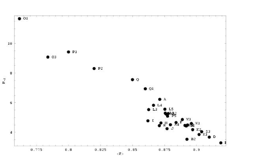
Figure 10: A scatter plot showing the correlation of a pair of output parameters, $P_{-2}$ against $\bar{F}$ for various simulations. Simulations O1, O3, P1, P2, Q1, Q and K3 all have 150 kpc cells. Simulations with small boxes, such as A4, B2 and B in the lower right, will have $P_{-2}$ values that are significantly too small. The simulations show a strong correlation, with larger $P_{-2}$ for more absorption.

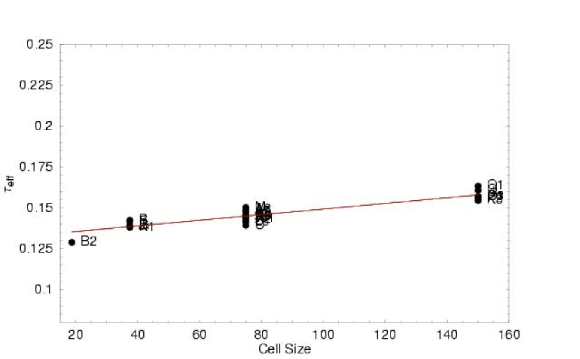
Figure 18: As Fig. 16 but for $\tau_{eff}$ against cell size.

As in T04b we use $b$-values from Figure 10 of Kim et al. (2001), at redshifts $z=1.61$, 1.98 and 2.13. We use their sample A that includes lines with $12.5<$ log N_HI $<14.5$ cm^-2 and errors of $<25$% in both N_HI and $b$. The sample has 286 lines, from $1.5<z<2.4$, and shows no evolution. The mean redshift is 2.00. In Fig. 18 of T04b we showed that the distribution of these lines is very similar to that of lines in simulation B and to the function in Eqn. (5) when

$$\mbox{$b_{\sigma}$}=23.6\pm 1.5\rm~{}\rm km/s.$$ (11)

6.3 Published Flux Power

At least four papers present measurement of power on relevant scales: McDonald et al. (2000, M00a), C02b, K04e and M04a. The first three measure power on the scales of most interest to us, $0.01<k<0.1$ s/km, but we have limited overlap with the SDSS spectra in the fourth reference because our typical boxes are small compared to the smallest scale set by the intermediate spectral resolution.

Unfortunately there is no agreement on a standard definition for flux power in the literature. C02b discuss options and K04e label three quantities that we can take the power of: F1, F2 and F3. F1 gives the power of the amount of the flux in units of the unabsorbed continuum level, or normalized flux. This natural definition is very sensitive to the mean amount of absorption. F2 gives reduced (not zero) sensitivity to the mean absorption because it is the power of the normalized flux, divided by the mean of the normalized flux over some arbitrary range, measured from one spectrum at a time, the average of many spectra together, or a model (see C02b §2.2). F3 avoids continuum fits, and is the power of the observed flux, in cgs units, divided by its mean. The differences are significant. From Kim et al. (2004a, Table 3) we see that P(F1)/P(F2) has a mean of 0.51, and it drifts systematically up and down from around 0.45 to 0.53 over the listed $k$ range. P(F3)/P(F2) has a mean of 1.03 at $0.0056<k<0.075$ s/km, and it rises to $>1.2$ at both smaller and larger $k$ values.

There are other significant problems with flux power. For real spectra, flux calibration errors can be larger than the photon noise, the continuum level errors are hard to estimate, and metal lines and Ly$\alpha$ lines of LLS contribute significant power. Samples are often small and biased to have excess or too little metal lines absorption. At $k>0.1$ s/km metals are about 50% of the signal, and there are no large published samples that are metal free. Moreover, there appear to be real differences between measured power values even when the same definitions were apparently used. With the simulated spectra the power is inaccurate because the boxes are often many times too small.

For these reasons we can not yet make definitive contact between the simulations and data. The uncertainties in the data may be larger than those in the simulations, including the external errors.

6.3.1 Flux Power From Kim et al 2004

We have scaled the power measurements from K04e to match our $z=1.95$ and to approximately remove the power from metal lines. Our definition of flux power matches F2 in Eqn. 3 of K04e. They list revised F2 at various $k$ values for samples with mean redshifts of $z=1.87$, 2.18 and 2.58 in Table 5 of Kim et al. (2004a). The F2 flux power is slightly lower at lower redshifts, with F2(1.87)/F2(2.18) typically 0.9 with a range of 0.7 – 1.1 for $-2<k<-0.8$ s/km. For each $k$ value that they list, we linearly interpolate in $log(1+z)$ between log PF2(1.87) and log PF2(2.18) to find log PF2(1.95). We do the same with relative errors (not log relative errors) that range from 15 – 50% at $k=0.001$ to $0.03$ s/km, and from 6 – 11% at larger $k$ values. F2 values changes rapidly with $k$ near $P_{-1}$: dropping a factor of 2 from $k=-1.0$ to $-0.9$. We list these quantities in Table 3.

Next we correct for metal lines. In Table 3 we list $f_{m}(k,z=2.36)=P_{metals}^{1D}(k)/P_{F1}^{1D}(k)$, the metal lines power as a fraction of the F1 power at a mean $z=2.36$ from Kim et al. (2004b, Fig. 3). We assume that a similar ratio would apply to F2, and we use a constant value of $f_{m}=0.0667$ for all $k<0.01$ s/km because we suspect that the error is larger than the fluctuations in their figure.

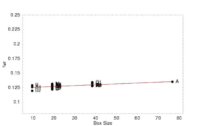
Figure 16: The output parameter $\tau_{eff}$ after scaling using the relations in Table 6 to scale to our standard parameters, listed in Table 7. We do not scale by the quantity shown on the horizontal axis, in this case box size.

We expect that $f_{m}$ increases as $z$ drops, because the total absorption from the low density IGM evolves faster than that from metal lines (T04b). McDonald et al. (2004a, Fig. 16) see a rapid change in power at $z<2.3$ compared to higher $z$ that may have the same origin. To correct for metal line power, we assume that the metal flux power does not change with redshift. First we find the total power at $z=2.36$ by interpolation in $log(1+z)$ between $logPF2(2.18)$ and $logPF2(2.58)$. Then we calculate the metal power $PF2M=f_{m}PF2(2.36)$. Finally we get the power in the low density IGM $PF2I(1.95)=PF2(1.95)-PF2M$. We list the PF2I(1.95) values in Table 3 and we list the power at the scales of $P_{-2}$, $P_{-1.5}$ and $P_{-1}$ in the top row of Table 1. The $1\sigma$ errors that we list ignore the error in the removal of the metal lines, and hence they are much too small for $P_{-1}$.

We do not know whether the metal power in the 13 QSOs where K04e fit metal lines is representative of their whole sample of 27 QSOs, and especially the QSOs that contribute to the $F2(1.85)$. There are three reasons why the $f_{m}$ values might underestimate the metal power on scales $k<0.04$ s/km.

First, the measurements in T04b indicate that $f_{m}$ is of order 0.26 on scales around 0.0006 s/km in a larger sample at $z=1.9$, larger than the $f_{m}$ values of 0.06 – 0.1 on scales $k<0.04$ s/km.

Second, at $z=1.9$ metal lines are 19% of all absorption in the Ly$\alpha$ forest. It is likely that metals account for a larger fraction of the power on all scales than they do of the absorption, because the clustering of metal lines on scales out to 600 km/s is extremely strong, and much easier to detect that the clustering of the Ly$\alpha$ in the Ly$\alpha$ forest (Sargent et al., 1980).

Third, K04e state that their sample contained only 4 sub-damped Ly$\alpha$ absorbers (DLAs) that they removed. This is less than we might expect in a typical sample of 27 QSOs, and hence we expect that $f_{m}$ could be significantly larger than the values that we list. A single LLS or DLA can contribute a lot of absorption and hence power.

6.3.2 Flux Power from Other Papers

McDonald et al. (2004c, section 1) noted possible systematic normalization errors and/or underestimation of the errors when they compared measurement from different papers. We find that the power in K04e and C02b agrees at $z=2.13$, but that the power in both McDonald et al. (2000) and McDonald et al. (2004c) is systematically lower, for no know reason.

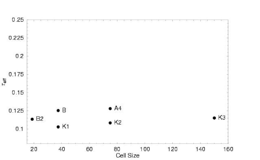
Figure 5: The variation of $\tau_{eff}$ with cell size. Simulations B2BA4 ($X_{228}$$=1.8$) all have the same parameters except for cell size, as do the K series ($X_{228}$$=3.3$). In all Figures the cell size is in comoving kpc for $h=0.71$.

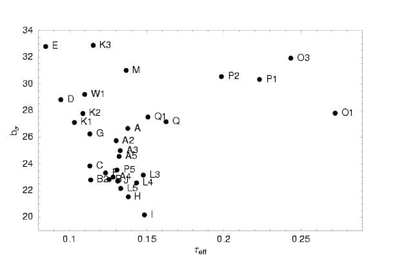
Figure 9: A scatter plot showing the correlation of a pair of output parameters, Line width parameter $b_{\sigma}$ against effective optical depth for various simulations. Cell size decreases to the lower left. Simulations O1, O3, P1, P2, Q1, Q and K3 all have 150 kpc cells. They are joined by M that has broad lines because it has low $\sigma_{8}$ and high $X_{228}$ values. K1, G, B, H and I all have 37.5 kpc cells while B2 has 18.75 kpc cells. For a given cell size, $b_{\sigma}$ increases as $\tau_{eff}$ decreases.

McDonald et al. (2000, Table 4) list flux power at $z=2.41$ from complete HIRES spectra of 1 QSO and partial spectra of 4 others. In Fig. 5c they show that metal lines have $f_{m}=0.57$ at $k=0.126$ s/km, more than the $f_{m}=0.39$ from K04e at $z=2.36$ for $k=0.1334$, but consistent considering the huge errors expected using so few QSOs. Kim et al. (2004b, Fig. 9) suggests that the M00 power is consistent with that of K04e at $z=2.35$. Croft kindly points out that M00 give the power of $F-\mbox{$\bar{F}$}$, where as $F2=(F-1)/\mbox{$\bar{F}$}$. Since power is proportional to the square of the signal, we should divide the power in M00 by $\bar{F}$² for comparison with F2. Using $\bar{F}$$=0.818$ for $z=2.41$ from M00 Table 1, this increases the M00 power by a factor of 1.494. We scaled the K04e F2 power, including metal lines but not the four sub-DLAs, to $z=2.41$ for the comparison. We list values in Table 4. The two look extremely similar on a log $k$ – log Power plot, but the systematic differences are much larger than the relative errors that we quote in Table 3. The M00 power is lower over most $k$ values, and the ratio PM00/PK04 is 1.04 at $P_{-2}$, 0.84 at $P_{-1.5}$ and 0.76 at $P_{-1}$. This result cast some doubt on our rescaling of the M00 power, because the K04e power agrees with C02b.

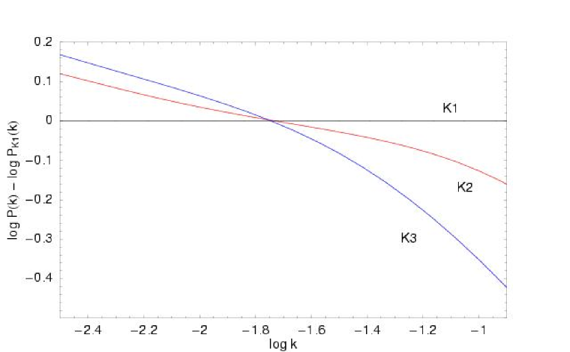
Figure 7: The effect of cell size on flux power. The 1D flux power as a function of wave number k in s/km. The simulations shown have identical input parameters except for cell size. We have divided the power by that for simulation K1 that has the smallest cell size (37.5 kpc). With smaller cell size the small scale power increases while that on large scales decreases.

In their Table 7 C02b give flux power of F2 from their subsample A of 9 HIRES spectra that cover $1.7<z<2.3$ with a mean $z=2.13$. Kim et al. (2004a, Fig 7) shows that the K04e power at $z=2.04$ is approximately 1.5 times that of C02b at $z=2.13$. However, when we compare to the K04e power at $z=2.18$, or a rescaling to $z=2.13$, we find excellent agreement for $-2.5<k<-1.2$ s/km, with the exception of the C02b power at $k=0.00437$ s/km that is obviously too low from Table 7 of C02b. At $k>-1.2$ s/km we see more power in C02b because the C02b sample of HIRES spectra had lower S/N, and perhaps also more metal lines than the K04e sample.

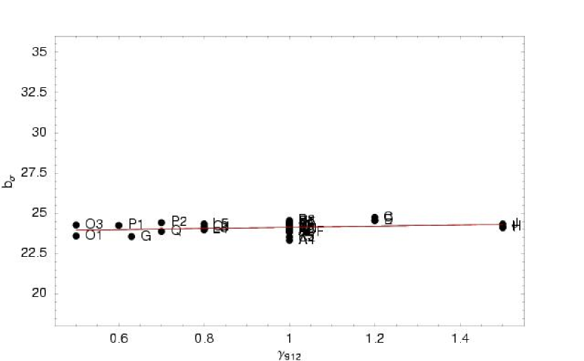
Figure 23: As Fig. 16 but for $b_{\sigma}$ against $\gamma_{912}$.

M04a gives power at $k<0.02$ for $z=2.2$ from SDSS spectra. The $P_{F}$ tabulated in their Table 3 is power of $F2$. Their Fig. 23 shows that the power decreases smoothly with $z$, but with some large deviations for the $2.2$ measurements at $k=$ 0.01413 and 0.01778 s/km, the two largest $k$ values. For $k=0.00891$ to 0.01122 s/km, we fit a line to their $\log P_{F}$ (values taken from their Table 3) as a function of $\log k$ and extrapolated the result to $z=1.95$. We found that a straight line produced an excellent fit to $\log P_{F}$ vs. $\log k$ between $2.2<z<3.8$, so we expect that the small extrapolation from $z=2.2$ to $z=1.95$ is probably valid. We find $P_{F2}(k=0.00891,z=1.95)=7.28$ km s^-1, and $P_{F2}(k=0.01122,z=1.95)=6.11$ km s^-1. Doing a linear interpolation in $k$ between these two points gives $P_{F2}(k=0.01,z=1.95)=6.7$ km s^-1. M04a quote relative errors of approximately 0.044 on the power around this $k$ at $z=2.2$. The error on the power that we extrapolate to $z=1.95$ will be larger, by perhaps 30% giving $\pm 0.38$. This value, $6.7\pm 0.38$ s/km includes metal lines, yet it is a factor of 0.76 smaller, $2\sigma$, than the value that we interpolated from K04e, $8.8\pm 1.0$ s/km. We give both values near the top of Table 1.

6.4 New Measurement of Flux Power

We were tempted to make our own measurements of the flux power, to help resolve definition and normalization uncertainty, and also because we can remove from the small sample both the metal lines and the Ly$\alpha$ of LLS.

The data set we use consists of high resolution quasar spectra taken with the Keck HIRES (FWHM $=8$ km s^-1) and VLT UVES (FWHM$=4.3$ km s^-1) spectrograph. The sample we use consists of 6 spectra, with QSO emission redshifts ranging from 1.71 to 2.65. The HIRES data were obtained as part of the effort to measure the mean cosmic baryon density $\Omega_{b}h^{2}$ by comparing the ratio of deuterium to hydrogen with the predictions of primordial nucleosynthesis (e.g. Kirkman et al., 2003). The details of observational techniques, data reduction and continuum fitting are described in more detail in the above paper.

We fitted the metal and Ly$\alpha$ lines in all these spectra, and we made artificial noise free spectra containing only the Ly$\alpha$ lines with log N_HI$<17.2$ cm^-2. We used these noise free fits because some of the spectra are low S/N, and we know from Viel et al. (2003) that line profiles contain most of the power information. We do not claim that this will give an accurate power measurement, but we were able to use exactly the same algorithms on these spectra and those from simulations.

The region we use from each spectrum spans the wavelength range from 1000 km s^-1 redward of Ly$\beta$ to 3000 km s^-1 blueward of Ly$\alpha$, to avoid the effect of any ionizing radiation arising due to the close proximity to the quasar. The redshifts of the Ly$\alpha$ forest data ranges from 1.52 to 2.61. In general, signal to noise ratio (S/N) increases with wavelength due to CCDs sensitivity and atmospheric extinction. The QSO redshift, signal to noise ratio (S/N) and length of each spectra is shown in Table 5.

As in Croft et al. (2002), we scale the optical pixel depths by a factor of ${(1+z)^{4.5}}$ to the mean z of the sample in order to mitigate the effects of evolution. To reduce evolution we used spectra covering only redshifts 1.7 – 2.3 and to reduce differences in normalizations and windowing we divided each spectrum into segments of length 0.1 in $z$, the same length as the simulated spectra. We had a total of 34 segments, with slightly more at z greater than 2.0.

We calculated the flux power spectrum of each QSO segment and averaged them. To help others to compare with our results, we give the normalization now. Given a spectrum of length L and number of points N, we define the power spectrum as the ${DFT\times L/N^{2}}$ where L is in units of km/s and $DFT$ is the dimensionless output from the Discrete Fourier Transform. This normalization matches that of Croft et al. (2002), and the F2 of K04e. When we divided by the mean flux, we took the mean for each QSO separately, as did K04e.

We call this new power spectrum PJ05. In Table 2 we give the coefficients of the polynomial representation (§5.3), and we show this polynomial and compare it to simulations in §10.1. We list values from the polynomial fit near the top of Table 1.

We again see systematic differences between power spectra. PJ05 is larger than PF2I at all $logk<-1.1$ s/km, and smaller otherwise. The ratio PJ05/PF2I is 1.27 at $P_{-2}$, 1.33 at $P_{-1.5}$ and 0.90 at $P_{-1}$, although the difference is only significant around $P_{-1.5}$ where PJ05-PF2I = $5\sigma$(PF2I). We understand the sense of the differences. The spectra that we used for PJ05 often have lower S/N and larger continuum level errors than those used in PF2I. This would tend to make PJ05 larger on large scales. In addition, for PJ05 we used fits to spectra rather than spectra, and this leads to a lack of power on small scales, from the lack of photon noise and weak Ly$\alpha$ forest lines. For these reasons we do not consider PJ05 to be as accurate as PF2I, and we do not know how to give errors on PJ05. However, PJ05 does suggest that the methods that we use on the simulated spectra should give results similar to both PJ05 and PF2I.

7 Convergence Tests

In this section we examine the effects of the box size and then the cell size (resolution) on each of the parameters that we measure from the simulated spectra: the mean flux, b-values and the flux power spectrum. We would like the parameters measured from the simulations to have errors that are smaller than those of the data. We find that surprisingly large boxes, $>100$ Mpc, and small cell size ($<30$ kpc) are required. While we have no single simulation with these ideal parameters, we do explore a range that shows us how to scale the results from practical smaller simulations to those we expect from such ideal simulations.

7.1 Box Size

We need a large box size to contain large scale power. Simulations in the A series used identical inputs except for the box size. The pair W1 and K2 also differ only in box size, but they have $X_{228}$$=3.3$ that makes them hotter than the A series with less small scale power and wider lines.

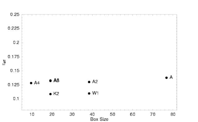
Figure 2: The change in $\tau_{eff}$ with box size. The A simulations ($X_{228}$$=1.8$) all have all the same parameters except for box size, as do the pair K2W1 ($X_{228}$$=3.3$). The points and labels for A3 and A5 lie on top of each other. In all Figures the box size is in comoving Mpc for $h=0.71$.

In Fig. 2 we plot the $\tau_{eff}$ for these simulations. As the box size doubles in the A series; from 9.6 to 19.2, 38.4 and to 76.8 Mpc; the mean flux decreases by 0.0040, then $-0.0023$, then 0.0066. A2 shows a different behavior, but the size of the effect is less than two times the random error for a single set of 25 spectra: $\sigma=0.0028$ (§5.4). We can ignore A5 since it uses the same box as A3. The effect of doubling the box size is smaller than the measurement error, but not by much, and the convergence is slow. The change in $\bar{F}$ for K2W1 shows the same trend as A3A.

From Table 1 and Fig. 3 we see that the $b_{\sigma}$ values increase with box size. The increase is seen in both the A series and with W1K2, and it is a large increase of 1.7 km/s (6.7%) from 19.2 to 76.8 Mpc. As we double the box size starting from 9.2 Mpc in the A series, the $b_{\sigma}$ increases by factors of 1.086, 1.030 and 1.036; again a slow convergence.

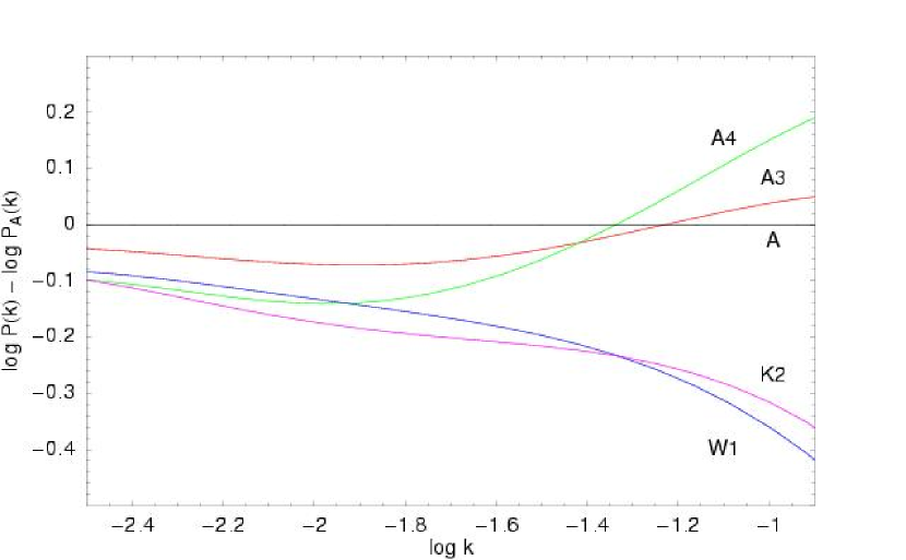
Figure 4: The effect of box size on flux power. The 1D flux power as a function of wave number k in s/km. We have divided the power spectra by that for the simulation with the largest box, A. As box size increases, from A4 (9.6 Mpc) to A3 (19.2 Mc) to A (76.8 Mpc), the power at $logk>-1.3$ s/km (small scales) decreases, while that on larger scales increases as the boxes contain more large scale matter power (§2.2). K2 (19.2 Mpc) and W1 (38.4 Mpc) show the same trend, but tilted because we divided their flux power by A. We show the power at smaller $k$ values than is justified by the box sizes to help illustrate the trends and differences. The 19.2 Mpc boxes include only modes $n>2$ for $logk=-2$ s/km (§5.3). In all plots involving power, $k$ is in units of s/km for our standard model, and the power is the 1D flux power of the quantity that Kim et al. (2004b, Eqn. 3) call F2.

The 1D flux power spectra change shape as the box size increases. In Fig. 4 we show the 1D flux power from simulations A3, A4, W1 and K2 in units of the power from simulation A. The A series differ in box size alone. We see that the larger boxes lead to reduced power at $k>0.05$ s/km for the A series with 75 kpc cells and $X_{228}$$=1.8$. We see a similar trend for W1K2, shifted lower on the plot and tilted because we have divided by the flux power of A. We note that simulation A2 seems to have flux power that is out of order with their respective series. We suspect that this may be some error, but we do not delete the entries because we could not find any errors.

The changes in $P_{-1}$ as the box size doubles are factors of 0.772, 0.852 and 1.075. For the first two increases in box size, these changes are larger than the changes in $b_{\sigma}$. However going from the 38.4 Mpc to the 76.8 Mpc the $P_{-1}$ increases rather than decreases. The general inverse relation between $b_{\sigma}$ and $P_{-1}$ follows from Viel et al. (2003, Fig. 2).

Simultaneously with the decrease in $P_{-1}$ we see $P_{-2}$ increase with increasing box size. $P_{-2}$ increases with the box size because the larger boxes contain more long modes. The W1K2 shows similar trends for $b_{\sigma}$ and the flux power.

The precise effect of the loss of large modes is complicated when we compare simulations. Nearly all boxes have the same seeds. The overall density pattern is similar in all such boxes, but the $k$ ranges corresponding to the pattern change with the box size.

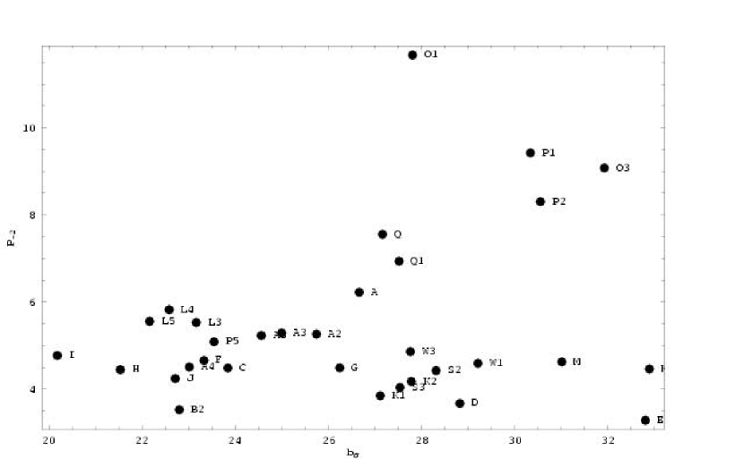
Figure 13: A scatter plot showing the correlation of a pair of output parameters, $P_{-2}$ against $b_{\sigma}$ for various simulations. Simulations O1, O3, P1, P2, Q1, Q and K3 all have 150 kpc cells and have larger $P_{-2}$ values, above the other simulations on the plot. The remaining simulations show a slight decrease of $P_{-2}$ with increasing $b_{\sigma}$.

The $P_{-1}$ drops as the box size increases because increased matter power leads to decreased flux power on small scales. As we enlarge the box, keeping the cell size and all cosmological and astrophysical parameters constant, more long modes enter. The power increases on all scales, and especially those that were near the size of the smaller boxes. As the simulation evolves the matter power increases on all scales leading to larger matter power on all scales in larger boxes by $z=1.95$. McDonald (2003, Fig. 10a) and McDonald et al. (2004c, Fig. 13) both show that an increase in matter power on all scales leads to a decrease in the 3D flux power on scales $k>$ 0.01 – 0.02 s/km at $z=2.2$. According to these papers the reduction of small scale 3D flux power power is from the increase in nonlinear peculiar velocities, a fingers-of-god effect. The 1D flux power then also decreases on small scales as the matter power increases.

7.2 Cell Size or Resolution

The cell size has to be small enough to resolve the structures in the IGM that change the output parameters. The K series simulations differ only in the cell size, as do the series A4, B and B2. The K series reach our smallest cell size, 18.75 kpc, but they are all in 9.6 Mpc boxes. The A4BB2 series are in 19.2 Mpc boxes, with $X_{228}$$=3.3$, but they stop at 37.5 kpc cells.

In Fig. 5 we show $\tau_{eff}$ against cell size. The mean flux increases by 0.006 and 0.005 as the cell decreases from 150, to 75 to 37.5 kpc. These changes are larger than we would like, and imply that cells of less than 37.5 kpc might be needed to measure the mean flux to within 0.01.

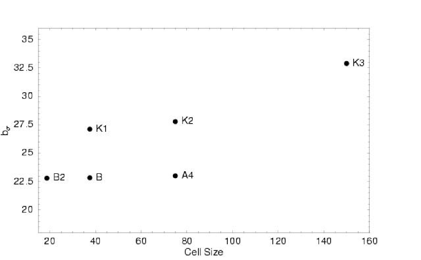
Figure 6: The variation of $b_{\sigma}$ with cell size. Simulations B2BA4 ($X_{228}$$=1.8$) all have the same parameters except for cell size, as do the K series ($X_{228}$$=3.3$).

In Fig. 6 we show the decrease in $b_{\sigma}$ with decreasing cell size. The effect is large for cells $>75$ kpc, but small for smaller cells.

Fig. 7 shows the flux power for the K series simulations with different cell size. The K series show simple patterns: as the cell size decreases, from K3 to K2 to K1, the power on small scales $k>0.018$ s/km increases while that on larger scales decreases. We did not expect the large scale power to decrease, because these simulations all began with the same large scale 3D matter power. Perhaps this is an effect of long modes missing from all the boxes; modes that are better sampled with the smaller cells.

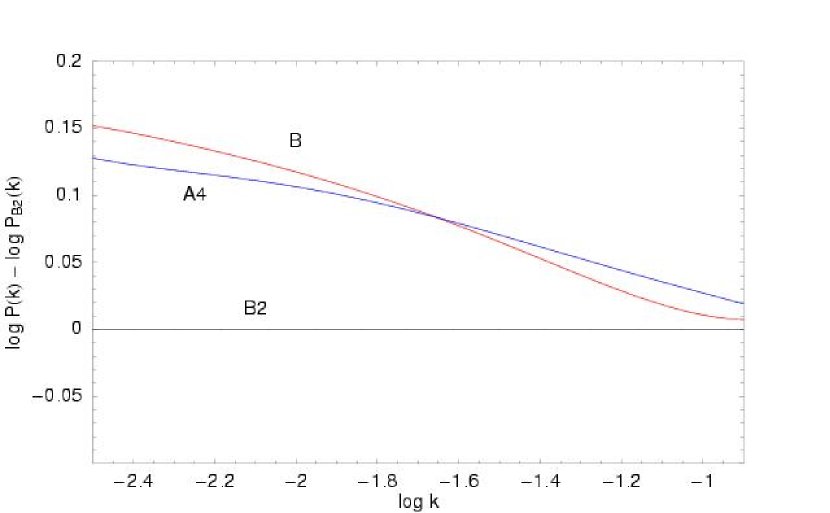
Figure 8: The effect of cell size on flux power. The 1D flux power as a function of wave number k in s/km. The simulations shown have identical input parameters except for cell size. We have divided the power by that for simulation B2 that has the smallest cell size (18.75 kpc).

Fig. 8 shows the effect of cell size on flux power for A4BB2. The results looks rather different from the K series, and we suspect some error, perhaps in the power for simulation B.

For comparison, McDonald et al. (2004c, Section 2.2) use 14.29 Mpc boxes with 55.8 kpc cells, and they test for resolution convergence with a 7.14 Mpc box and 55.80 and 27.90 kpc cells. At $z=2.125$ the flux power is lower in the lower resolution simulation by about 0.2% from $0.01<k<0.05$ s/km, after they adjusted the redshift of reionization, and 1% larger before the correction. The differences are several times larger at $k=0.1$ s/km.

While (Bryan et al., 1999) found that 37.5 kpc is sufficient to resolve the Ly$\alpha$ forest at $z=3$ and we prefer smaller cells at $z=2$ because the density contrast is larger.

When we compare simulations with differing box and cell size we will apply the systematic corrections that we derive in §9.

8 Correlation of Measured Output Parameters

In this section we examine the correlations between the five output parameters that we measure from the simulated spectra: the mean flux, b-values and the flux power on three scales.

In Fig. 9 models with the large 150 kpc cells, O1, O3, P1, P2, Q, Q1 and K3 are on the upper right. They are joined by M that has broad lines because it has low $\sigma_{8}$ and high $X_{228}$ values. We will see these same simulations stand apart from others in many subsequent plots. The remaining simulations show larger $b_{\sigma}$ values for smaller $\tau_{eff}$. This is not the trend expected from line saturation that has the opposite sense.

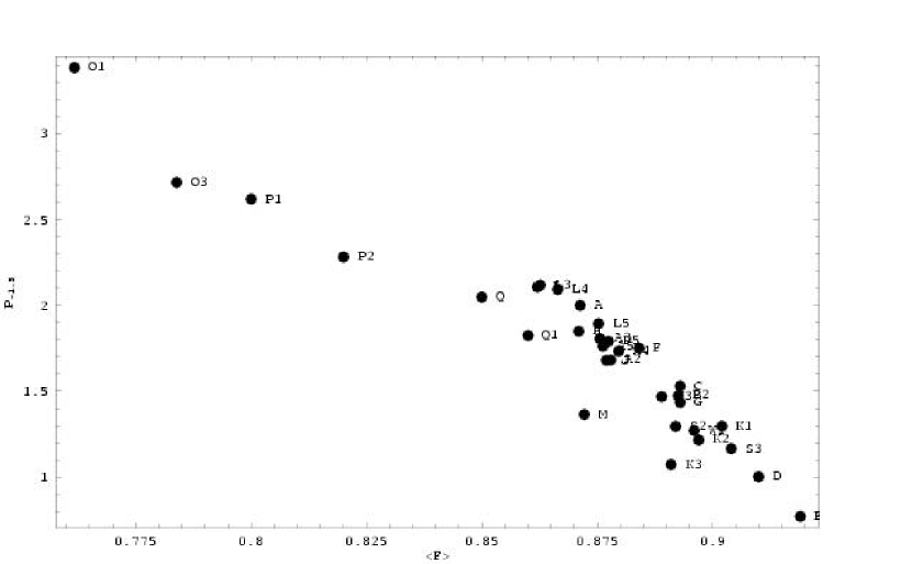
Figure 11: A scatter plot showing the correlation of a pair of output parameters, $P_{-1.5}$ against $\bar{F}$ for various simulations. Simulations O1, O3, P1, P2, Q1, Q and K3 all have 150 kpc cells and lie on a diagonal line below and to the left of the other simulations. They are joined by M that has broad lines because it has low $\sigma_{8}$ and high $X_{228}$ values. The remaining simulations show a strong correlation, with larger $P_{-1.5}$ for more absorption.

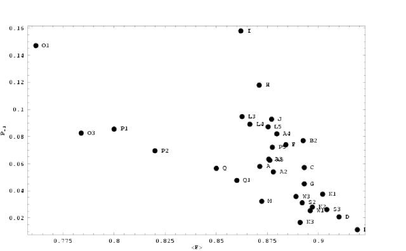
Figure 12: As Fig. 11 but for $P_{-1}$. Simulations O1, O3, P1, P2, Q1, Q and K3 all have 150 kpc cells and lie on a diagonal line below and to the left of the other simulations. They are joined by M that has broad lines because it has low $\sigma_{8}$ and high $X_{228}$ values. Simulations in the upper right (I, H, J, F, C, G, K1) all have 37.5 kpc cells, while B2 has 18.75 kpc cells. For a given cell size the simulations show a correlation, with larger $P_{-1}$ for more absorption. There is more scatter than for $P_{-2}$ and $P_{-1.5}$ because factors such as cell size and $X_{228}$ have a larger effect on $P_{-1}$ than on $P_{-2}$ and $P_{-1.5}$.

It is well known that for a given matter power the flux power is a strong function of the mean flux ((Croft et al., 2002; Gnedin & Hamilton, 2002; Viel et al., 2004a); also §1 of T04b). The flux power increases as the mean flux decreases, by Parseval’s theorem, because a lower mean flux corresponds to more flux variance. In Fig. 10 we see that the effect remains strong for $P_{-2}$, even though the flux power that we use, coming from F2, is less sensitive to the mean flux than other definitions. The models on the upper left all have the large 150 kpc cells. We see a similar trend for $P_{-1.5}$ in Fig. 11. However, in Fig. 12 we see much more scatter for $P_{-1}$, because other factors have a large effect on the power on small scales.

The trends in Figs. 10 and 12 suggest that we should increase $P_{-2}$ by 6% and $P_{-1.5}$ by 5% when we the decrease the $\bar{F}$ by 0.0051 to correct the absorption missing at the start of each spectrum.

Viel et al. (2003, Fig. 1) show that the flux power for all three $k$ values; $P_{-2}$, $P_{-1.5}$ and $P_{-1}$; is extremely similar to the power of a random arrangement of a sample of real absorption lines fitted with Voigt profiles. When they artificially increased all $b$-values, the power spectrum shifts to larger $k$ in their Fig. 2. In the band of $P_{-1}$ they find that doubling all $b$-values, making all lines broader, gives about 8 times less power. Halving all $b$-values gives 5 times less power. We expect to readily see a strong correlation between $P_{-1}$ and $b_{\sigma}$ and we expect to be sensitive to much smaller changes. The band $P_{-2}$ is less sensitive to changes in the $b$-values, and in the opposite sense to $P_{-1}$, while the $P_{-1.5}$ is insensitive to $b$-values.

In Fig. 13, 14 and 15 we show how the flux power depends on $b_{\sigma}$. In all three Figs. simulations O1, O3, P1, P2, Q and Q2; all with the 150 kpc cells; lie in the upper right and can be ignored. We see that power decreases as $b_{\sigma}$ increases for all three power bands. The effect is small for $P_{-2}$, intermediate for $P_{-1.5}$, and strong for $P_{-1}$, as expected. Since our simulations differ in various input parameters, and we did not change $b$-values explicitly, we should not conclude that the trends that we see for $P_{-1.5}$ and $P_{-2}$ differ from the results of Viel et al. (2003, Fig. 2).

8.1 Extra Information in the Flux Power

It is interesting to ask whether the flux power contains any information that is not in the mean flux and b-values. We ask this because the flux power is strongly correlated with both the mean flux and b-values, and the dispersion in flux power seems to contain approximately two degrees of freedom. We can think of one of these as controlling the amplitude and the second the shape, or the ratio $P_{-2}$/$P_{-1}$. The answer will depend on the level of accuracy required.

A result in McDonald et al. (2004c) also hints that the flux power is contained in the mean flux and $b_{\sigma}$. They state that they can derive the mean flux to better than 1% error when they match their observed flux power to simulations. Since they use intermediate resolution spectra that do not resolve lines, their flux power contains only the longer scale information on b-values, and their results will be sensitive to their spectral resolution.

While it is clearly the case that the flux power on the largest scales is strongly correlated with the matter power that we parameterize with $\sigma_{8}$ and $n$, on small scales the flux power is most strongly effected by the factors that determine the mean flux and $b$-values. These factors include the temperature which we parameterize with $X_{228}$ and the combination of parameters that set the ionization, especially $\gamma_{912}$. The power that we measure at $k>0.01$ s/km is not a good measure of the matter power because of the importance of these other factors.

We have not tried to determine whether, to the level of accuracy of our simulations, the mean flux and $b_{\sigma}$ contain essentially all the information that is in the flux power on small scales. This comparison would be difficult because we are most interested in the largest scales, but our boxes are missing power on these scales, and the power on these scales is effected by our choice to start the simulated spectra at the cell with the lowest density in each box.

9 Scaling Laws

We now determine the scaling relationship between the two groups of parameters, the input to the simulations and the outputs that we measured from the simulated spectra. We will give scaling relationships between individual inputs and outputs. We vary only one input at a time, noting the values of all the others that we keep fixed. We find that the cross terms are small, allowing us to vary five different inputs simultaneously and obtain accurate predictions for the outputs.

There has been much work on scaling in the literature, including recent work by McDonald (2003); McDonald et al. (2004c); and Bolton et al. (2004). We will not attempt to compare our simulation results with theirs because we typically differ in numerous input parameters, including the corrections for box and cell size.

In Table 6 we list functional forms and the parameters that describe the scalings. We list five input variables in the first column, and two output variables, $\tau_{eff}$ and $b_{\sigma}$. The table entries give the value of the output parameter that we expect as a function of each of the five input parameters. If a parameter is not explicitly used, then these scalings give the values expected using the default value for our standard model, listed in Table 7. This standard also includes the corrections for starting the lines of sight at random positions in the box, rather than the lowest density point. As elsewhere in this paper the box size $L$ is in comoving Mpc and cell size $C$ in comoving kpc, both for $h=0.71$.

To scale an output to different input parameters, we multiply the output by the relevant scaling factor. We give relations for two of the five outputs, $\tau_{eff}$ and $b_{\sigma}$. For example, simulation A gave $\tau_{eff}$$=0.13778$ for cell size $C=75$ kpc. Let us rescale this $\tau_{eff}$ to the value that we would expect from a simulation with $C=18.75$ kpc. We multiply 0.13778 by $\tau_{eff}$$(C=18.75)/$$\tau_{eff}$$(C=75)$ = 0.9352, where $\tau_{eff}$$(C)=0.132828+0.00016748C$, giving $\tau_{eff}$= 0.12885. We can calculate similar correction factors for both $\tau_{eff}$ and $b_{\sigma}$, to scale using all five input parameters for which we give scaling relations.

The scalings work very well within the range of parameters given in Table 1, and we can use them to scale an output by one input parameter, two parameters or even all five inputs. To rescale by more than one input parameter we simply apply the product of the relevant correction factors.

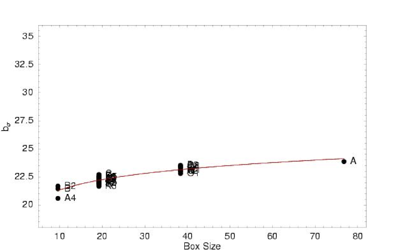
Figure 17: As Fig. 16 but for $b_{\sigma}$ against box size.

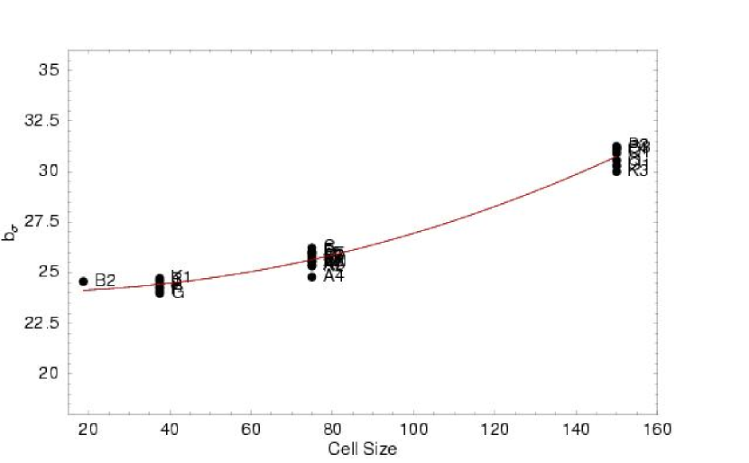
Figure 19: As Fig. 16 but for $b_{\sigma}$ against cell size.

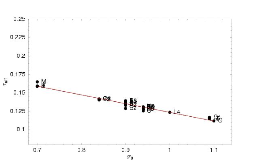
Figure 20: As Fig. 16 but for $\tau_{eff}$ against $\sigma_{8}$.

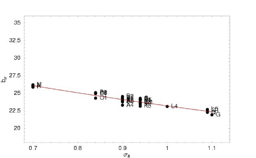
Figure 21: As Fig. 16 but for $b_{\sigma}$ against $\sigma_{8}$.

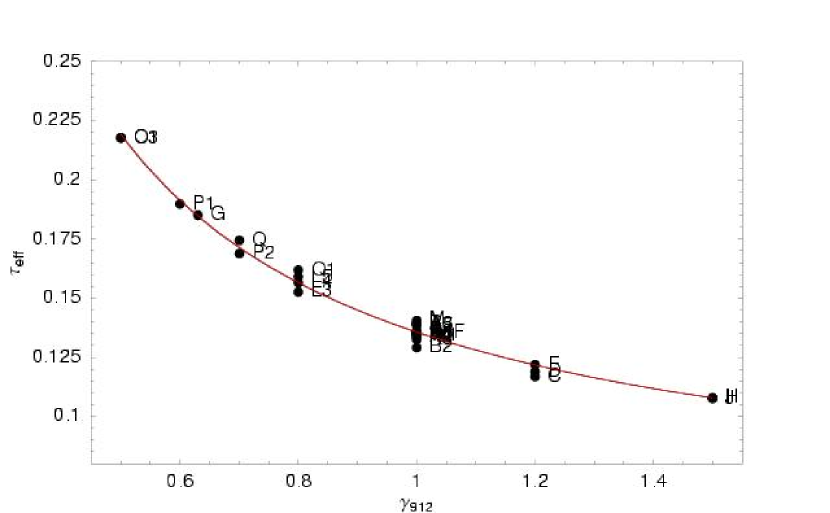
Figure 22: As Fig. 16 but for $\tau_{eff}$ against $\gamma_{912}$.

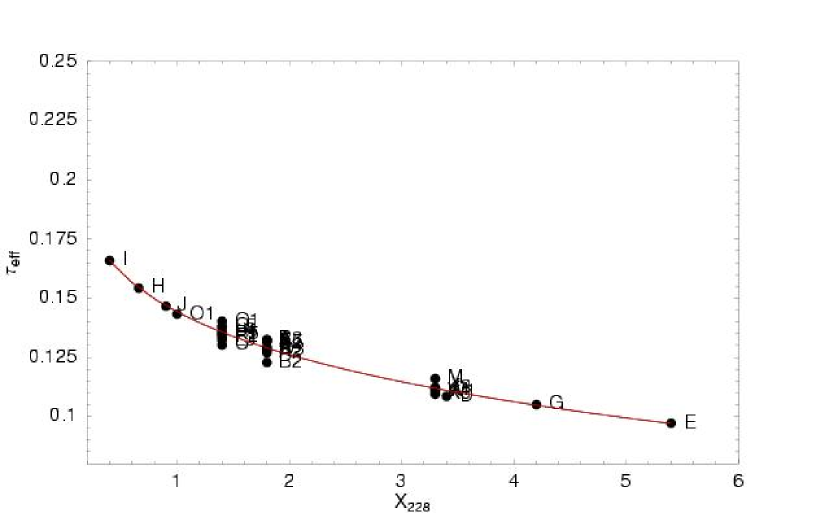
Figure 24: As Fig. 16 but for $\tau_{eff}$ against $X_{228}$.

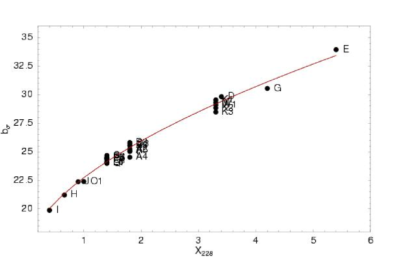
Figure 25: As Fig. 16 but for $b_{\sigma}$ against $X_{228}$.

The scaling relations presented in Table 6 are shown in Figures 16 – 25. Each Figure shows either $\tau_{eff}$ or $b_{\sigma}$ as a function of one of the input parameters: box size ($L$), cell size ($C$), $\sigma_{8}$, $\gamma_{912}$, or $X_{228}$. In each figure, $\tau_{eff}$ and $b_{\sigma}$ have been rescaled to our standard model values for all of the input parameters except the one being displayed as the independent variable in that figure. There are three points to take away from our scaling figures: (1) Our scalings work remarkably well over a wide range of input parameters. (2) The scalings are self consistent. (3) Our procedure of applying multiplicative correction factors in succession to rescale for more than one change in input parameters works well, implying that the cross terms are small.

There is nothing fundamental about using the scaling relations to produce multiplicative correction factors. While the multiplicative correction factors are defined such that they must give correct results when only rescaling by a single input variable, we use the multiplicative factors because they also work well when rescaling by more than one input. This need not have been the case, and the fact that the multiplicative rescalings work so well indicates that the full equations giving $\tau_{eff}$ and $b_{\sigma}$ are separable in $L,C,\mbox{$\sigma_{8}$},\mbox{$\gamma_{912}$},$ and $X_{228}$ with very small cross terms between the input parameters.

In Fig. 26 we show the values we predict for $b_{\sigma}$ and $\tau_{eff}$ when we scale the output parameters from each simulation to the standard model. A measure of the accuracy of the scalings is the dispersions in these scaled values: the mean $\tau_{eff}$$=0.13539$ with standard deviation $\sigma($$\tau_{eff}$$)=0.0027$, while the mean $b_{\sigma}$$=24.139$ km s^-1 with $\sigma($$b_{\sigma}$$)=0.33$ km s^-1. The typical error from the use of the scaling relations is then 1.4% for $b_{\sigma}$, and 2.0% for $\tau_{eff}$, equivalent to an error on the mean flux $\bar{F}$ of 0.27%. We can predict the $b_{\sigma}$ and $\bar{F}$ that we will obtain from simulations with errors four times smaller than the errors on the measurements from the data that we presented in §6.1 and 6.2. This suggests that the measurements from the simulations could be more accurate than the data, provided the calibrations are reliable.

The scalings should not be used for extrapolations, because the functional forms may be unreasonable outside the range of our models. We also note that the values for the parameters in a given equation are strongly correlated. A wide range is allowed for a scaling parameter in Table 6 when the range of the input parameter in our simulations is small. For example, for $\gamma_{912}$ we used 0.5 – 1.2 in different simulations, and the range allowed for the exponent in the equation $\tau_{eff}$$=0.0517116+0.0845752\mbox{$\gamma_{912}$}^{-1}$ is much larger than you might expect. We choose $-1$ because this provides a good fit, but $-0.8$ and $-1.2$ also fit well. We can neither confirm nor refute the exponent of $-1.44$ that Bolton et al. (2004, Eqn. 9) found in a different way, by post processing their simulations to change the $\tau_{eff}$ value, although we have more to say on this in §9.1.

9.1 Effect of Specific Scalings

We now discuss some of the results and compare to prior literature. We do not repeat our discussion of box and cell size in §7.

Both $h$ and $\Omega_{b}h^{2}$ are well known from other measurements (Freedman et al., 2001; Kirkman et al., 2003; Spergel et al., 2003) and so the few simulations that we ran to explore their effects cover only a small range.

We discussed how the $\bar{F}$ and $\tau_{eff}$ depend on $\Omega_{b}$ and $h$ in T04b §12.1.2 and 12.1.4. In Table 1 we give output parameters for simulations S2K2S3 that vary in $\Omega_{b}$ and $h$ simultaneously such that $\Omega_{b}h^{2}$ is approximately constant. Their output parameters vary by approximately the errors on the relevant data.

Since with various assumptions $\tau\propto h^{-1}(\Omega_{b}h^{2})^{2}$ (Rauch et al. 1997, Eqn. 17, Bolton et al. 2004), we can use the quantity

$$Y=\mbox{$\tau_{eff}$}h/(\Omega_{b}h^{2})^{2}\propto\mbox{$\tau_{eff}$}/\tau,$$ (12)

to make an approximate estimate of how $\tau$ depends on $\tau_{eff}$. We find that Y increases as $\tau_{eff}$ drops, but by only 4% from simulation S2 to S3. This trend is fit with with $\tau\propto$$\tau_{eff}$^-1.32, consistent with Bolton et al. (2004, Eqn. 9) who found an exponent of $-1.44$. Although the changes are very small, and unlikely to be reliable, the relation does significantly decrease the dispersion in the Y parameter: $\sigma(Y)/Y=$2% drops to 0.5% if we use $\tau_{eff}$ ^-1.32 in place of $\tau_{eff}$ in the Y definition. However, this result is illustrative and not definitive, since changes in $\Omega_{b}$ also lead to changes in the gas temperature (Gardner et al., 2003; Tytler et al., 2004) and Jeans smoothing (Tytler et al., 2004, Section 12.1.2), both leading to changes in $\tau_{eff}$ that are not included in the equations that we used here. The scaling of $\tau_{eff}$ with $\gamma_{912}$ in Table 6 is derived from simulations that include these astrophysical effects and should be more reliable.

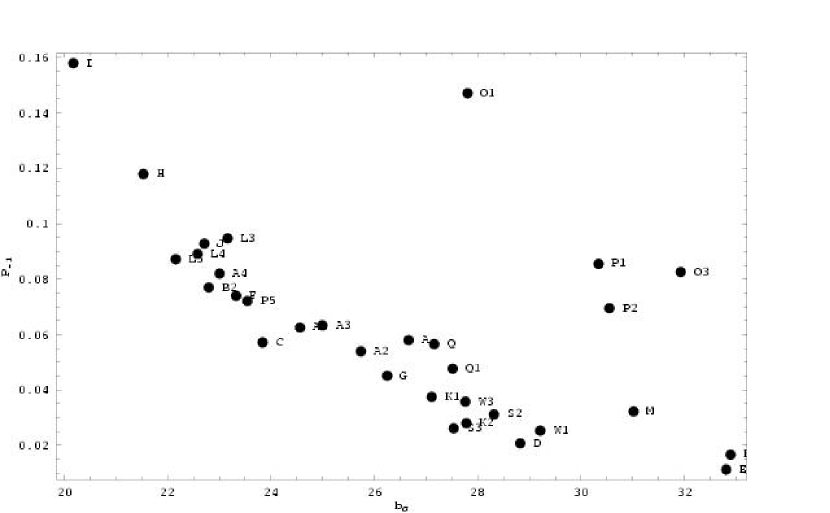
Figure 15: As Fig. 13 but for $P_{-1}$.

We do have two sets of simulations with slightly differing $\Omega_{m}$ and $\Omega_{\Lambda}$ values for flat models. Larger $\Omega_{m}$ corresponds to larger $\bar{F}$, and smaller $P_{-2}$ and $b_{\sigma}$. However, the two sets show different trends for $P_{-1.5}$ and $P_{-1}$. In Fig. 15 we saw that $P_{-1}$ and $b_{\sigma}$ are typically anticorrelated, as for K3 and V, and contrary to the trend for T and K2. Although the change in $b_{\sigma}$ is larger than the measurement error, we are not convinced that this difference is robust.

9.2 Effect of ${\sigma_{8}}$

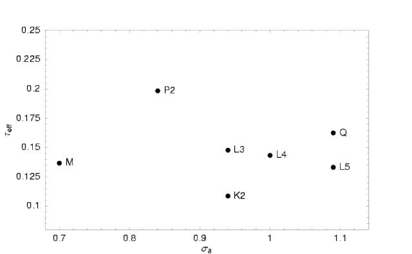
Figure 27: Output parameter $\tau_{eff}$ as a function of input $\sigma_{8}$ for three sets of simulations that differ in $\sigma_{8}$ alone. MK2 have 75 kpc cells and $X_{228}$$=3.3$. The L series have 75 kpc cells and $X_{228}$$=1.4$. P2Q have 150 kpc cells and $X_{228}$$=1.4$.

In Fig. 27 we show the raw $\tau_{eff}$ for three sets of simulations: MK2, L3L4L5 and P2Q. For each set the $\tau_{eff}$ drops with increasing $\sigma_{8}$ as we noted in T04b.

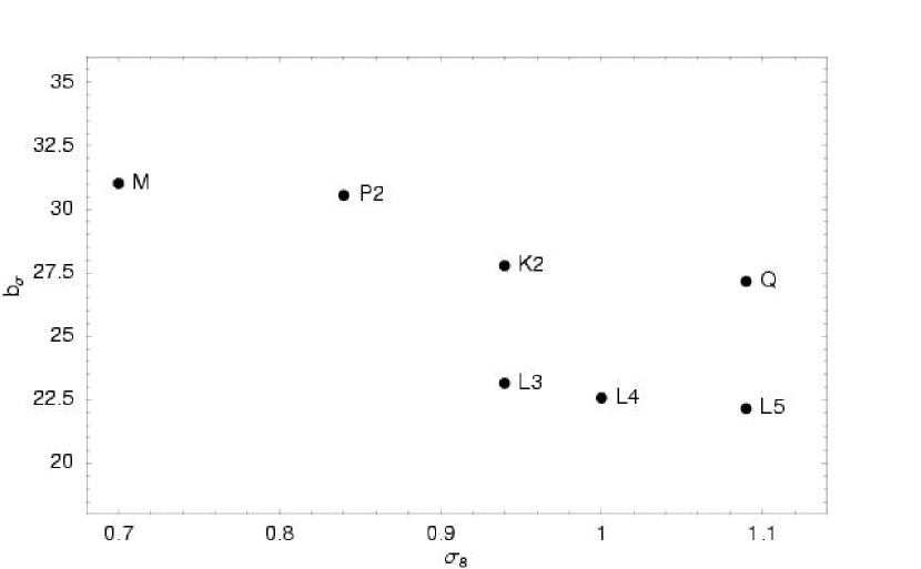
Figure 28: Output parameter $b_{\sigma}$ as a function of input $\sigma_{8}$ for three sets of simulations that differ in $\sigma_{8}$ alone. MK2 have 75 kpc cells and $X_{228}$$=3.3$. The L series have 75 kpc cells and $X_{228}$$=1.4$. P2Q have 150 kpc cells and $X_{228}$$=1.4$.

In Fig. 28 we show that larger $\sigma_{8}$ gives smaller $b_{\sigma}$, as was noted by Bryan & Machacek (2000, Fig. 7) and Theuns et al. (2000, Fig. 5). Theuns et al. (2000) saw the trend in a portion of their simulated spectrum, but the VPFIT software that they used to obtain the b-value distribution failed to show the change because more lines were added instead of wider ones.

The set UQ1 is different because its $P_{-2}$ and $P_{-1.5}$ values drop with increasing $\sigma_{8}$, the opposite trend from the other sets, perhaps because the cell size is large.

9.3 Effect of ${\gamma_{912}}$

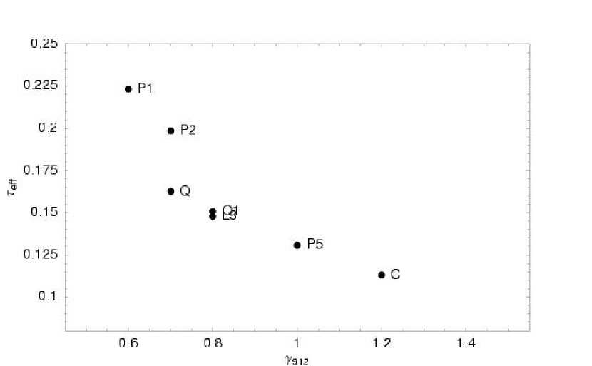
Figure 29: Output parameter $\tau_{eff}$ as a function of input $\gamma_{912}$ for three sets of simulations that differ in $\sigma_{8}$ alone. L3P5C have 75 kpc cells, $X_{228}$$1.4$ and $\sigma_{8}$$=0.94$. P1P2 have 150 kpc cells and $X_{228}$$1.4$ and $\sigma_{8}$$=0.84$. QQ1 have 150 kpc cells and $X_{228}$$1.4$ and $\sigma_{8}$$=1.09$.

In Fig. 29 we show the $\tau_{eff}$ for three sets of simulations, each of which differ only in $\gamma_{912}$. All three sets show less absorption and smaller $\tau_{eff}$ for larger $\gamma_{912}$, as expected (Croft et al., 2002).

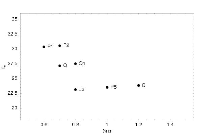
Figure 30: As Fig. 29 but for $b_{\sigma}$.

In Fig. 30 we show the $b_{\sigma}$ for three sets of simulations, each of which differ only in $\gamma_{912}$. We see a slight increase in $b_{\sigma}$ with $\gamma_{912}$.

9.4 Effect of $X_{228}$ 

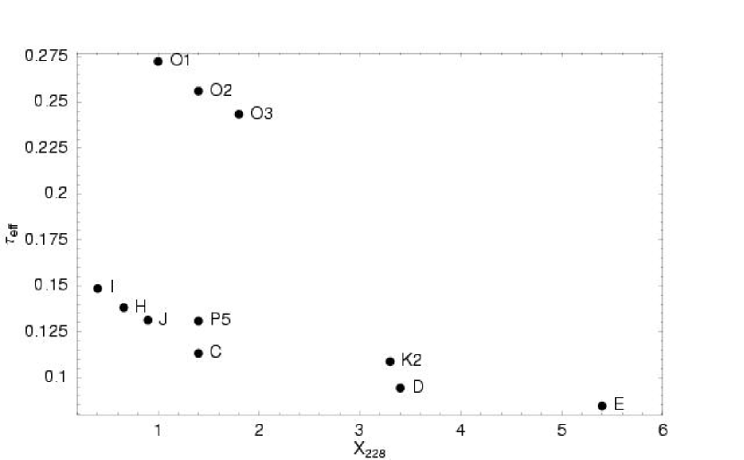
Figure 31: Output parameter $\tau_{eff}$ as a function of input $X_{228}$ for four sets of simulations that differ in $X_{228}$ alone. IHJ have 37.5 kpc cells, $\gamma_{912}$$=1.5$ and $\sigma_{8}$$=0.70$. CDE have 37.5 kpc cells, $\gamma_{912}$$=1.2$ and $\sigma_{8}$$=0.94$. P5K2 have 75 kpc cells, $\gamma_{912}$$=1.0$ and $\sigma_{8}$$=0.94$. O1O2O3 have 150 kpc cells, $\gamma_{912}$$=0.5$ and $\sigma_{8}$$=0.84$.

In Fig. 31 we show the $\tau_{eff}$ for four sets of simulations, each of which differ only in $X_{228}$. All sets show less absorption in hotter models, as we expect.

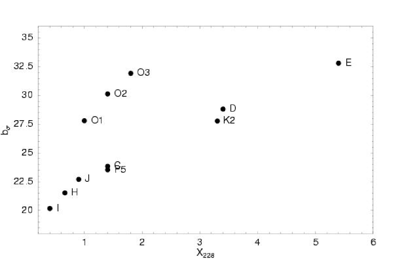
Figure 32: As Fig. 31 but for $b_{\sigma}$.

In Fig. 32 we show how $b_{\sigma}$ depends on $X_{228}$ for the same four sets as in Fig. 31. We see that the hotter models have larger $b_{\sigma}$.

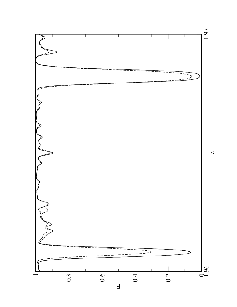
Figure 33: Sample spectra for two simulations I and J which differ only in the $X_{228}$ parameter. The solid line is simulation I, $X_{228}$ = 0.4 and the dotted line is simulation J, $X_{228}$ = 0.9.

In Fig. 33 we show an example of the effect of changing $X_{228}$ on simulated flux spectra. As we expect, increasing the $X_{228}$ results in more ionization and thus in less absorption. Accordingly, the flux spectra shows lines closer to the unabsorbed value of 1.0. However, it is not obvious from this segment of spectrum, of length $\Delta z=0.01$, that simulation J has larger $b_{\sigma}$ than simulation I.

9.5 Comparison to Bolton

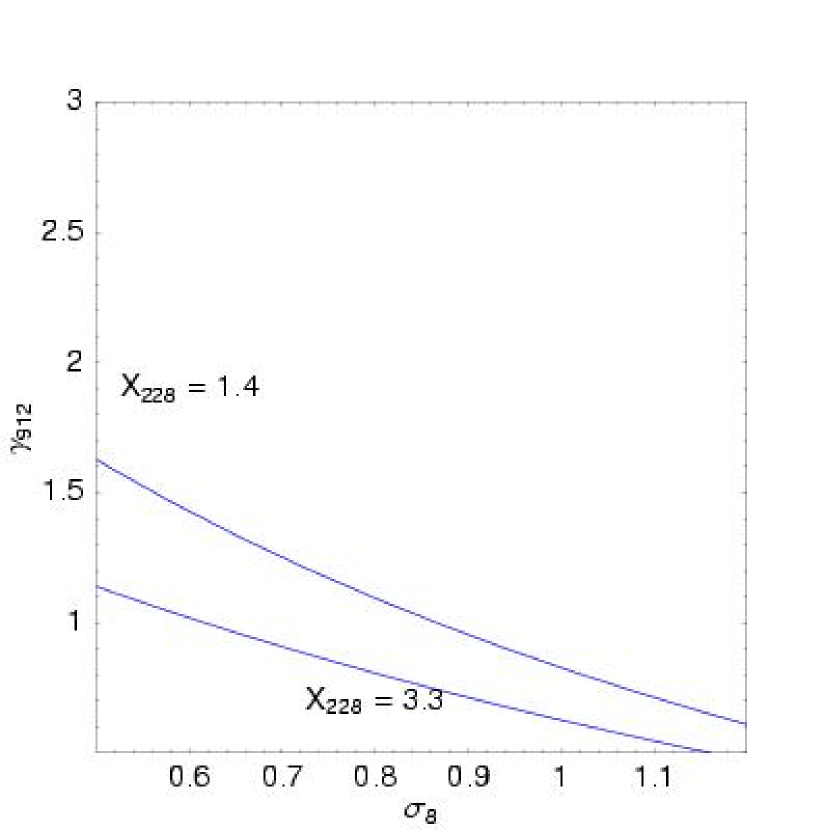
Figure 34: The lines show the value of $\gamma_{912}$ required to give the observed mean flux at $z=1.95$ for a range of $\sigma_{8}$ values and our standard model. All our simulations have $\sigma_{8}$ in the range 0.7 – 1.1, and hence outside this range the scaling relations are extrapolated and the errors are unknown and possibly large. A value of $X_{228}$$=1.4$ was used in Fig. 16 of T04b while Bolton et al. (2004, Fig. 3 right) used 3.3. The models with $X_{228}$$=3.3$ are all too hot and ruled out by the widths of absorptions lines, measured with either $b_{\sigma}$ or $P_{-1}$. The models with $X_{228}$$=1.4$ are too hot for $\sigma_{8}$$<0.94$ and too cold for $\sigma_{8}$$>0.94$. Models that are consistent with both the mean flux and the line widths have $X_{228}$ increasing with $\sigma_{8}$, as shown in Fig. 37.

In Fig. 34 we show the $\gamma_{912}$ that gives the observed $\bar{F}$ as a function of $\sigma_{8}$. As we expected, hotter models need less $\gamma_{912}$. This Figure is similar to Fig. 16 of T04b and Fig. 3 (right) of Bolton et al. (2004), with five exceptions. First, T04b used $X_{228}$= 1.4, while Bolton et al. (2004) used $X_{228}$= 3.3. This difference explains why the curve in Bolton et al. (2004) lies well below that in T04b for $\sigma_{8}$= 0.84 and 0.7. A second differences is with the scalings used to correct for box and cell size. In T04b we did not make any such corrections, and the simulations that we used had $L=19.2$ Mpc and 75 kpc cells. Bolton et al. (2004) did correct for box and cell size, as we do here for Fig. 34, but we expect there to be some difference in these corrections because they are hard to estimate. A third difference is in the redshift. We now work at $z=1.95$, where as T04b and Bolton et al. (2004) were for $z=1.90$. A fourth difference is that we derived the approximate scalings that we used in T04b from simulations with $\sigma_{8}$ = 0.7 – 1.09. Outside this $\sigma_{8}$ range the scaling relations that we showed were extrapolated, and can readily have large errors. We can not calibrate these errors because all our simulations still have 0.7 – 1.1. Values for $\sigma_{8}$ outside this range are of little cosmological interest. Since the main purpose of Fig. 34 is to aid comparison with past work, and we know that we should increase $X_{228}$ as $\sigma_{8}$ varies, we again show scalings extrapolated to a wider range of $\sigma_{8}$ values. We see that T04b was relatively accurate at $\sigma_{8}$$>0.9$ where the scalings were small, and that our new scaling relations show that we overestimated the $\gamma_{912}$ required at $\sigma_{8}$$<0.8$. The fifth difference is with the other cosmological parameters. Here and in T04b we used $\Omega_{b}h^{2}$$=0.02218$, $\Omega_{m}$$=0.27$, $h=0.71$ and $n=1$, while Bolton et al. (2004) used $\Omega_{b}h^{2}$$=0.02400$, $\Omega_{m}$$=0.26$, $h=0.72$ and $n=0.95$. The points from Bolton et al. (2004) lie between our curves for $X_{228}$$=3.3$ and 1.4 for $\sigma_{8}$$<1$. They are 1.13 times higher than our $X_{228}$$=3.3$ curve for $\sigma_{8}$$=0.5$, rising smoothly to 1.27 times higher by $\sigma_{8}$$=1.2$. This difference might be largely explained by the different $n$ values, since for smaller $n$, a smaller $\sigma_{8}$ value has the same matter power on relevant scales.

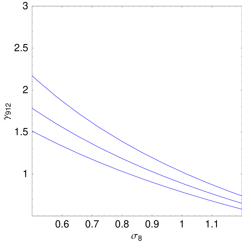
Figure 35: The $\gamma_{912}$ required to give DA = 0.885, 0.875, and 0.865 for various $\sigma_{8}$ in our standard model with $X_{228}$$=1.4$.

Fig. 35 is similar to Fig. 34 but drawn for the three DA values given in T04b. We see that the range of $\gamma_{912}$ allowed by the error in the measurement of DA of 0.01 is larger than that shown in Fig. 16 of T04b. The present figure superseded that given in T04b.

10 Joint Determination of Cosmological Parameters

In general we can not break the degeneracy between $\sigma_{8}$ and $X_{228}$ using only mean flux, small scale flux power and b-values with the accuracies assumed in this paper. We can find models that fit all these observables simultaneously for a wide range of $\sigma_{8}$ from 0.7 – 1.1. We did not explore a larger range, and we did not examine the small differences between these models.

We can break this degeneracy using some other information on $\sigma_{8}$ from the large scale flux power (T04b) or from some other measure of large scale clustering, such as the galaxy distribution or the CMB. The large scale flux power is helpful because it responds in a different way to changes in $X_{228}$ than does the small scale power that we have discussed. The power spectrum changes shape with changes in $\sigma_{8}$ and $X_{228}$. McDonald (2003, Fig. 10a) and McDonald et al. (2004c, Fig. 13) both show how the flux power responds to small changes in various parameters. Increasing $\sigma_{8}$ causes more 3D flux power on large scales, less on small scales, and no change near $k=0.03$ s/km at $z=2.2$. On large scales the flux power is proportional to the amplitude of the mass power spectrum, or $\sigma_{8}^{2}$, as Croft et al. (1998) assumed and McDonald et al. (2000, App. C) proved.

We can readily distinguish models that have differing $\sigma_{8}$ because they will have different large scale power. The large scale power, or equivalently, the fluctuations in the mean flux on large scales, gives $\sigma_{8}$ directly, avoiding the complications found in small scales. Unfortunately we can not explore large scale power with our existing simulations because most of our boxes are too small. However, in T04b we showed that the variation in the mean flux in spectral segments with length $\delta z=0.1$ was similar to the variations seen in our largest simulation, A, and consistent with $\sigma_{8}$$=0.90^{+0.13}_{-0.16}$ for $n=0.95$.

In the next section we give the sets of parameters that are consistent with data. We will treat $\sigma_{8}$ as a control variable, but we could have used some other parameter.

10.1 A Concordance Model for the Lyman-$\alpha$ forest at z = 1.9

For a given $\sigma_{8}$ and other cosmological parameters, we can estimate $\gamma_{912}$ and $X_{228}$. In Figs. 36, 37 and 38 we show the pairs of values that give the observed $\bar{F}$ and $b_{\sigma}$ at $z=1.95$ for our standard model. We do this by starting at our standard simulation and using our scaling relations to calculate the change in the input parameters necessary to match the two observables. We then have two equations in two unknowns. We then solve for the pair of values that would have matched the observed data for some value for the third parameter; for example, we can find values for $\gamma_{912}$ and $X_{228}$ which result in a match for some value for $\sigma_{8}$. We do not expect any significant error arising from the implicit assumption that the scaling laws between two of our input parameters do not depend on the third parameter as we have shown this to be true in §9.

For $\sigma_{8}$ in the range 0.8 – 1.0 the $\gamma_{912}$ and $X_{228}$ are both similar to unity, implying that the photoionizing spectrum is similar to that predicted by Madau et al. (1999). For $\sigma_{8}$$=0.9$ and the other standard model parameters from Table 7 we find $\gamma_{912}$$=1.0$ and $X_{228}$$=1.26$. The $\gamma_{912}$$=1.0$ implies a mean ${\Gamma=1.329\times 10^{-12}}$ s^-1 and a minimum $J_{912}(z=2)=0.30\times 10^{-21}$ $\mathrm{ergs}\mathrm{\ cm}^{-2}\mathrm{\ s}^{-1}\mathrm{\ Hz}^{-1}\mathrm{\ sr}^{-1}$ using Hui et al. (2002, Eqn. 3), or $J_{912}(z=2)=1.7\times 10^{-21}$ $\mathrm{ergs}\mathrm{\ cm}^{-2}\mathrm{\ s}^{-1}\mathrm{\ Hz}^{-1}\mathrm{\ sr}^{-1}$, if we assume a hard spectrum with a volume emissivity spectrum of slope $-0.5$. This may be compared to recent measurements of the ionizing rate. A recent analysis of the proximity effect gave ${\Gamma=1.9_{-1.0}^{+1.2}}\times 10^{-12}$ s^-1 averaged from z = 1.7 to 3.8 (Scott et al., 2000). Steidel et al. (2001) measured the specific intensity to be $J_{912}=1.2\pm 0.3\times 10^{-21}$ $\mathrm{ergs}\mathrm{\ cm}^{-2}\mathrm{\ s}^{-1}\mathrm{\ Hz}^{-1}\mathrm{\ sr}^{-1}$ from Lyman Break Galaxies at $z\sim 3$ and Hui et al. (2002) assume a functional form for the specific intensity to convert this to $\Gamma=1.89_{-0.99}^{+1.21}\times 10^{-12}$ s^-1. McDonald & Miralda-Escudé (2001) compare observed mean transmitted flux with that of simulated spectra to infer the intensity of the ionizing background. They find $\Gamma=0.65\pm 0.1\times 10^{-12}$ s^-1 at z = 2.4.

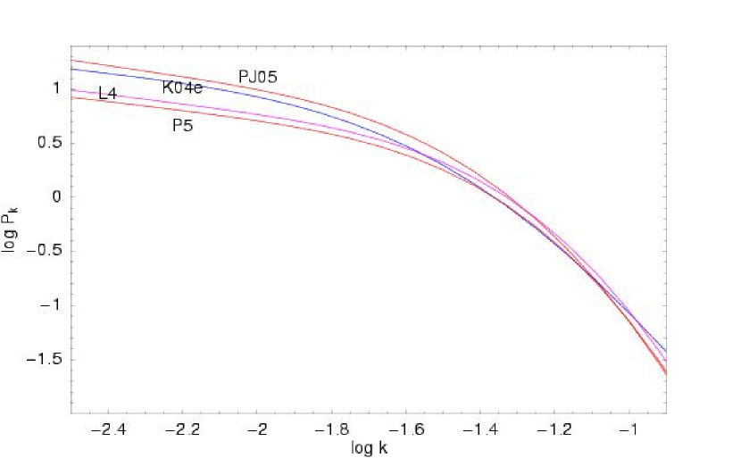
Figure 39: The flux power spectrum of data compared with the flux power spectrum from simulations L4 and P5, all at $z=1.95$. The spectrum labelled K04e is PF2I from Table 3, and the spectrum labelled PJ05 is our estimate of the $z=1.95$ power spectrum from the high resolution data in Table 5. Both K04e and PJ05 are the power of the low density IGM, with the contributions from Ly$\alpha$ of LLS and metal lines removed. We gave polynomial fits to these power spectra in Table 2. There is good agreement between the data and the simulations at $\log k>-1.4$ s/km, but the simulations have too little power on larger scales or smaller $k$ values. The lack of large scale power may be because the boxes are too small. We show the power at smaller $k$ values than is justified by the box size to help illustrate the trends and differences. Both L4 and P5 have 19.2 Mpc boxes that include only modes $n>2$ for $logk=-2$ s/km (§5.3).

In Fig. 39 we compare the power in simulations L4 and P5 to the measurements from K04e and our own measurement that we call PJ05. Both the measurements are for the low density IGM, with the signal from the Ly$\alpha$ lines of LLS and metal lines removed. The power in PJ05 is larger than that in K04e by approximately 25% at $logk<-1.3$ s/km then at $logk>-1.1$ s/km the PJ05 power becomes smaller. These errors are smaller than the differences between other measurements that we discussed in §6.3. We selected these two simulations because they gave unscaled $\bar{F}$ and $b_{\sigma}$ values, those in Table 1, that are similar to measurements. We see that the power in these simulations is indeed close to the data for $logk>-1.4$ s/km, indicating that the flux power spectrum on these small scales is well described with two parameters, such as $\bar{F}$ and $b_{\sigma}$. There appears to be little additional information in the small scale flux power spectrum.

On larger scales the power in the simulations is less than the measured power of the data. This may simply be the lack of large scale power put into the small 19.2 Mpc boxes. In Fig. 4 we saw that simulations in 19.2 Mpc boxes show less flux power than those in larger boxes on the same scales: $k<-1.4$ s/km, but we have not determined whether the magnitude of the lack of power from the boxes is enough to match the data. There will also be excess power in the data, especially at $logk<-2$ s/km, because the error in the continuum fits has not been subtracted.

The Ly$\alpha$ forest is very sensitive to $\sigma_{8}$, $\gamma_{912}$ and $X_{228}$. In Table 8 we show the expected error in our ability to compute $\tau_{eff}$ using our scaling relations. Here we assume that the scaling relations are free of errors, which means that we ignore errors in the corrections for box and cell size and we ignore the errors in the data that we used to derive the scalings. We consider only the gradients of the scaling relations. In the second column of Table 8 we give nominal prior values with errors, based on Table 7 of T04b. The entries in Table 8 supersede the last three rows in Table 7 of T04b. The third column of Table 8 gives the derivatives of our scaling relations evaluated at our standard model parameters, and the fourth column gives that derivative times the error on the prior value. The values in the fourth column are similar in size to the error in our measurement of DA in T04b, and given here in Eqn. (10). If we knew all the cosmological parameters in Table 7 without error, with the exception of one of $\sigma_{8}$, $\gamma_{912}$ or $X_{228}$, then we could measure that last parameter with an error similar to the error listed on the prior.

The main impediment to extracting cosmological information from the Ly$\alpha$ forest is not the sensitivity, but the rather large uncertainties in the astrophysical parameters $\gamma_{912}$ and $X_{228}$. Instead, the small scale information that we have discussed in this paper provide the best constraints on $\gamma_{912}$ and $X_{228}$, and when we have optically thick simulations we will be able to convert $X_{228}$ into a constraint on the ionizing spectrum.

11 Conclusion

We have explored the relationships between several cosmological and astrophysical parameters that effect the Ly$\alpha$ forest in hydrodynamic simulations. We have used 40 hydrodynamical cosmological simulations of the $z=1.95$ Ly$\alpha$ forest to measure the background radiation amplitude and the matter power amplitude. Both the data and simulations now support high accuracy. The HIRES and UVES spectra allow better continuum fits and better removal of metal lines and Lyman limit systems resulting in a mean flux measurement with an error of about 1%. The simulations used include not only gravitational effects, but also hydrodynamical effects as well as the effects of non-equilibrium chemistry of the baryons and the effects of a background ionizing radiation field. We did not rescale the output of the simulations to different temperatures. Instead we ran complete simulations to explore different UV background intensity and heating rates. We made corrections for the finite box size and resolution of our simulations.

We agree with other authors (Hui & Gnedin, 1999; Mandelbaum et al., 2003; McDonald et al., 2004a; Seljak et al., 2004; Viel et al., 2004b) that the careful comparison of large, well calibrated sets of simulations and data allow the extraction of both cosmological and astrophysical information from the Ly$\alpha$ forest.

We found that the simulations required to give the required accuracy are much larger than one might have expected: box size $L>100$ Mpc and cell size $C<50$ kpc, corresponding to at least $2048^{3}$ cells, similar to, or more demanding than the recommendations of others; eg. Meiksin & White (2004) who recommend $L>35$ Mpc and $C<$ 42 – 85 kpc at $z>3$. We find that boxes must be large enough to include modes two orders of magnitude larger than the filaments in the Ly$\alpha$ forest, much larger than those that have been used in nearly all prior work, a point made by Barkana & Loeb (2004). These simulations must also simultaneously have small cell size because larger cells give inaccurate absorption statistics, as we saw for our simulations with 150 kpc cells. However, once we resolve the Ly$\alpha$ forest, box size becomes the most critical parameter.

We have found that different output parameters are correlated. When we compare the $P_{-1}$, b-values and mean flux we find that we have only two independent degrees of freedom, to the level of accuracy of this study. We can predict the third parameter, in our case the power spectrum at $logk>-1.5$ s/km, from the other two.

We find that the mean flux and $b_{\sigma}$ are in many ways preferable to the flux power. The flux power is hard to measure because it is sensitive to continuum errors on intermediate and large scales, photon noise, metal lines and the Ly$\alpha$ of LLS on all scales and especially small scales for metals. The flux power is extremely sensitive to the mean flux and to redshift. There is no standard definition, and there are disagreements over values for apparently identical definitions.

We find scaling relations between the input and output parameters for the simulations. For the input parameters we explore $\sigma_{8}$, $\gamma_{912}$, $X_{228}$, box and cell sizes and for the output we explore $\bar{F}$ and $b_{\sigma}$. We find that the scalings are well determined and allow us to predict the outputs for any of our simulations, with errors of 0.3 km/s (1.4%) for $b_{\sigma}$, and 0.0027 (2.0%) for $\tau_{eff}$, equivalent to 0.0024 (0.27%) for $\bar{F}$ at $z=1.95$. We can also use the scalings to determine the input parameters that would yield a given pair of output parameters. The errors from the scalings are four times smaller than the errors on the measurements for the data that we presented in §6.1 and 6.2.

We use the scaling relations to scale our outputs to a standard model with $\Omega_{b}$= 0.044, $\Omega_{m}$= 0.27, $\Omega_{m}$= 0.23, $h=0.71$, $\sigma_{8}$= 0.9, $n=1.0$, $\gamma_{912}$$=1.4$, $X_{228}$$=1.0$, box size 76.8 Mpc and cell size 38.75 kpc. We also correct for the our mistaken choice of starting the simulated spectra at the lowest density point in the simulations.

We can break the degeneracy between $\sigma_{8}$, $X_{228}$ and $\gamma_{912}$ using large scale power or other data to fix $\sigma_{8}$. When we pick a specific $\sigma_{8}$ value, the simulations tell us the the $X_{228}$ and hence the temperature that we need to match the observed small scale flux power and b-values. We can then also find the H ionizing rate required to match the mean flux for that combination of $\sigma_{8}$ and $X_{228}$. Our scaling relations give the parameters for various $\sigma_{8}$ values.

This work demonstrates that precision measurements from the Ly$\alpha$ forest have excellent promise. We can make simulations and observations that are each accurate to several percent and we can make significant improvements with both.

Table 1: Input Parameters of the Hydrodynamic Simulations

Name	$\Omega_{b}$	$\Omega_{m}$	$\Omega_{\Lambda}$	$h$	$\sigma_{8}$	${\gamma_{912}}$	${X_{228}}$	L	N	Cell	$\bar{F}$	$P_{-2}$	$P_{-1.5}$	$P_{-1}$	${b_{\sigma}}$
PJ05											…	11.1	2.76	0.0755	…
M04a											…	6.7	…	…	…
Data											0.875	8.8	2.07	0.0841	23.6
$\sigma(Data)$											0.10	1.0	0.14	0.0067	1.5
A	0.044	0.27	0.73	0.71	0.90	1.0	1.8	76.8	${1024^{3}}$	75	0.8713	6.22448	2.00096	0.0580288	26.662
A2	0.044	0.27	0.73	0.71	0.90	1.0	1.8	38.4	${512^{3}}$	75	0.8779	5.26255	1.68276	0.0539609	25.741
A3	0.044	0.27	0.73	0.71	0.90	1.0	1.8	19.2	${256^{3}}$	75	0.8756	5.29052	1.80656	0.0633351	24.995
A5	0.044	0.27	0.73	0.71	0.90	1.0	1.8	19.2	${256^{3}}$	75	0.8762	5.23220	1.76246	0.0625227	24.560
A4	0.044	0.27	0.73	0.71	0.90	1.0	1.8	9.6	${128^{3}}$	75	0.8796	4.51003	1.73439	0.0820087	23.007
W1	0.044	0.27	0.73	0.71	0.94	1.0	3.3	38.4	${512^{3}}$	75	0.896	4.59288	1.2719	0.025351	29.212
K2	0.044	0.27	0.73	0.71	0.94	1.0	3.3	19.2	${256^{3}}$	75	0.897	4.17679	1.2170	0.028068	27.778
B2	0.044	0.27	0.73	0.71	0.90	1.0	1.8	9.6	${512^{3}}$	18.75	0.8925	3.52847	1.47406	0.0770033	22.7964
B	0.044	0.27	0.73	0.71	0.90	1.0	1.8	9.6	${256^{3}}$	37.5	0.8819	1.71394	4.62606	0.0789581	22.8300
A4	0.044	0.27	0.73	0.71	0.90	1.0	1.8	9.6	${128^{3}}$	75	0.8796	4.51003	1.73439	0.082008	23.007
K1	0.044	0.27	0.73	0.71	0.94	1.0	3.3	19.2	${512^{3}}$	37.5	0.902	3.85064	1.29774	0.0375323	27.110
K2	0.044	0.27	0.73	0.71	0.94	1.0	3.3	19.2	${256^{3}}$	75	0.897	4.17679	1.21702	0.0280679	27.778
K3	0.044	0.27	0.73	0.71	0.94	1.0	3.3	19.2	${128^{3}}$	150	0.891	4.46281	1.07452	0.0166946	32.892
L4	0.044	0.27	0.73	0.71	1.00	0.8	1.4	19.2	${256^{3}}$	75	0.8664	5.82605	2.0934	0.0890899	22.577
U	0.044	0.27	0.73	0.71	1.00	0.8	1.4	38.4	${256^{3}}$	150		6.36059	1.66403	0.0470178
L5	0.044	0.27	0.73	0.71	1.09	0.8	1.4	19.2	${256^{3}}$	75	0.8753	5.55675	1.89446	0.0871944	22.1579
Q1	0.044	0.27	0.73	0.71	1.09	0.8	1.4	38.4	${256^{3}}$	150	0.86	6.93897	1.82575	0.0477104	27.516
A	0.044	0.27	0.73	0.71	0.90	1.0	1.8	76.8	${1024^{3}}$	75	0.8713	6.22448	2.00096	0.0580288	26.662
A2	0.044	0.27	0.73	0.71	0.90	1.0	1.8	38.4	${512^{3}}$	75	0.8779	5.26255	1.68276	0.0539609	25.741
A3	0.044	0.27	0.73	0.71	0.90	1.0	1.8	19.2	${256^{3}}$	75	0.8756	5.29052	1.80656	0.0633351	24.995
B2	0.044	0.27	0.73	0.71	0.90	1.0	1.8	9.6	${512^{3}}$	18.75	0.8925	3.52847	1.47406	0.0770033	22.7964
B	0.044	0.27	0.73	0.71	0.90	1.0	1.8	9.6	${256^{3}}$	37.5	0.8819	1.71394	4.62606	0.0789581	22.8300
F	0.044	0.27	0.73	0.71	0.90	1.04	1.8	19.2	${512^{3}}$	37.5	0.884	4.65843	1.7522	0.074021	23.325
K1	0.044	0.27	0.73	0.71	0.94	1.0	3.3	19.2	${512^{3}}$	37.5	0.902	3.85064	1.29774	0.0375323	27.110
G	0.044	0.27	0.73	0.71	1.10	0.63	4.2	19.2	${512^{3}}$	37.5	0.893	4.48832	1.43529	0.0451349	26.246
I	0.044	0.27	0.73	0.71	0.70	1.50	0.40	19.2	${512^{3}}$	37.5	0.862	4.77332	2.10754	0.157915	20.174
H	0.044	0.27	0.73	0.71	0.70	1.50	0.66	19.2	${512^{3}}$	37.5	0.871	4.44712	1.85006	0.11792	21.531
J	0.044	0.27	0.73	0.71	0.70	1.50	0.90	19.2	${512^{3}}$	37.5	0.877	4.24435	1.68075	0.0928399	22.707
C	0.044	0.27	0.73	0.71	0.94	1.2	1.4	19.2	${256^{3}}$	75	0.893	4.48559	1.53054	0.0571994	23.842
D	0.044	0.27	0.73	0.71	0.94	1.2	3.4	19.2	${256^{3}}$	75	0.910	3.67275	1.00311	0.0207897	28.819
E	0.044	0.27	0.73	0.71	0.94	1.2	5.4	19.2	${256^{3}}$	75	0.919	3.28659	0.771793	0.0113551	32.806
P5	0.044	0.27	0.73	0.71	0.94	1.0	1.4	19.2	${256^{3}}$	75	0.8774	5.08876	1.79106	0.0721239	23.542
K2	0.044	0.27	0.73	0.71	0.94	1.0	3.3	19.2	${256^{3}}$	75	0.897	4.17679	1.21702	0.0280679	27.778
O1	0.044	0.27	0.73	0.71	0.84	0.5	1.0	38.4	${256^{3}}$	150	0.7617	11.6701	3.38596	0.147094	27.803
O2	0.044	0.27	0.73	0.71	0.84	0.5	1.4	38.4	${256^{3}}$	150	0.7741	10.8993	3.07758	0.108957	30.1342
O3	0.044	0.27	0.73	0.71	0.84	0.5	1.8	38.4	${256^{3}}$	150	0.7839	9.07688	2.71671	0.0826093	31.927
L1	0.044	0.27	0.73	0.71	0.70	0.8	1.4	19.2	${256^{3}}$	75					25.426
L2	0.044	0.27	0.73	0.71	0.79	0.8	1.4	19.2	${256^{3}}$	75	0.83	6.20307	2.51307	0.111913
L3	0.044	0.27	0.73	0.71	0.94	0.8	1.4	19.2	${256^{3}}$	75	0.8626	5.52899	2.11876	0.0947183	23.1608
L4	0.044	0.27	0.73	0.71	1.00	0.8	1.4	19.2	${256^{3}}$	75	0.8664	5.82605	2.0934	0.0890899	22.577
L5	0.044	0.27	0.73	0.71	1.09	0.8	1.4	19.2	${256^{3}}$	75	0.8753	5.55675	1.89446	0.0871944	22.1579
M	0.044	0.27	0.73	0.71	0.70	1.0	3.3	19.2	${256^{3}}$	75	0.8722	4.62589	1.36509	0.0322525	31.015
K2	0.044	0.27	0.73	0.71	0.94	1.0	3.3	19.2	${256^{3}}$	75	0.897	4.17679	1.21702	0.0280679	27.778
U	0.044	0.27	0.73	0.71	1.00	0.8	1.4	38.4	${256^{3}}$	150		6.36059	1.66403	0.0470178
Q1	0.044	0.27	0.73	0.71	1.09	0.8	1.4	38.4	${256^{3}}$	150	0.86	6.93897	1.82575	0.0477104	27.516
P2	0.044	0.27	0.73	0.71	0.84	0.7	1.4	38.4	${256^{3}}$	150	0.82	8.30225	2.28294	0.069514	30.5494
Q	0.044	0.27	0.73	0.71	1.09	0.7	1.4	38.4	${256^{3}}$	150	0.85	7.55325	2.04882	0.0565825	27.159
O2	0.044	0.27	0.73	0.71	0.84	0.5	1.4	38.4	${256^{3}}$	150	0.7741	10.8993	3.07758	0.108957	30.1342
P1	0.044	0.27	0.73	0.71	0.84	0.6	1.4	38.4	${256^{3}}$	150	0.80	9.42176	2.61947	0.0854846	30.3377
P2	0.044	0.27	0.73	0.71	0.84	0.7	1.4	38.4	${256^{3}}$	150	0.82	8.30225	2.28294	0.069514	30.5494
L3	0.044	0.27	0.73	0.71	0.94	0.8	1.4	19.2	${256^{3}}$	75	0.8626	5.52899	2.11876	0.0947183	23.1608
P5	0.044	0.27	0.73	0.71	0.94	1.0	1.4	19.2	${256^{3}}$	75	0.8774	5.08876	1.79106	0.0721239	23.542
C	0.044	0.27	0.73	0.71	0.94	1.2	1.4	19.2	${256^{3}}$	75	0.893	4.48559	1.53054	0.0571994	23.842
Q	0.044	0.27	0.73	0.71	1.09	0.7	1.4	38.4	${256^{3}}$	150	0.85	7.55325	2.04882	0.0565825	27.159
Q1	0.044	0.27	0.73	0.71	1.09	0.8	1.4	38.4	${256^{3}}$	150	0.86	6.93897	1.82575	0.0477104	27.516
S2	0.051	0.27	0.73	0.66	0.94	1.0	3.3	19.2	${256^{3}}$	75	0.892	4.42602	1.29656	0.031181	28.313
K2	0.044	0.27	0.73	0.71	0.94	1.0	3.3	19.2	${256^{3}}$	75	0.897	4.17679	1.21702	0.0280679	27.778
S3	0.038	0.27	0.73	0.76	0.94	1.0	3.3	19.2	${256^{3}}$	75	0.904	4.03904	1.16607	0.0262167	27.536
T	0.044	0.22	0.78	0.71	0.94	1.0	3.3	19.2	${256^{3}}$	75	0.887	4.48482	1.36005	0.0315291	28.671
K2	0.044	0.27	0.73	0.71	0.94	1.0	3.3	19.2	${256^{3}}$	75	0.897	4.17679	1.21702	0.0280679	27.778
K3	0.044	0.27	0.73	0.71	0.94	1.0	3.3	19.2	${128^{3}}$	150	0.891	4.46281	1.07452	0.0166946	32.892
V	0.044	0.32	0.68	0.71	0.94	1.0	3.3	19.2	${128^{3}}$	150	0.905	4.11799	1.15153	0.026181	27.318

Table 2: Polynomial Fit Coefficients to Simulation Flux Power Spectrum

Name	$B$	$A$	$C$	$E$	$F$	$G$
PJ05	1.726	43.709	42.008	15.075	2.407	0.144
A	2.048	55.103	49.214	16.433	2.440	0.136
A2	2.652	81.246	64.923	19.468	2.600	0.130
A3	2.635	77.822	62.260	18.678	2.495	0.125
A4	2.615	80.807	66.037	20.249	2.765	0.142
A5	2.006	57.992	53.459	18.466	2.839	0.164
B	1.916	56.461	54.123	19.469	3.122	0.188
B2	2.346	72.765	63.377	20.715	3.015	0.165
C	1.874	54.883	52.543	18.871	3.020	0.182
D	2.697	90.751	71.484	21.148	2.787	0.138
E	2.207	69.003	59.082	18.988	2.719	0.146
F	1.888	54.335	51.927	18.599	2.967	0.178
G	1.954	56.939	52.984	18.500	2.880	0.168
H	2.506	80.153	68.218	21.783	3.095	0.165
I	1.859	54.190	53.822	20.029	3.316	0.206
J	2.423	78.646	67.938	22.023	3.178	0.172
K1	1.949	57.636	53.391	18.538	2.866	0.166
K2	2.034	65.849	60.151	20.619	3.149	0.181
K3	1.617	54.038	54.058	20.286	3.394	0.213
L2	1.909	62.159	60.186	21.805	3.511	0.212
L3	2.078	56.175	50.878	17.243	2.599	0.147
L4	2.145	63.071	56.947	19.279	2.907	0.165
L5	3.375	89.469	61.666	15.949	1.837	0.079
M	2.835	116.928	92.016	27.194	3.579	0.177
O1	-1.261	-2.682	-2.017	-0.046	0.788	0.307
O2	0.566	21.158	29.526	15.214	3.498	0.303
O3	2.738	66.863	50.661	14.339	1.801	0.085
P1	-1.315	-2.664	-2.285	-0.359	0.697	0.316
P2	-1.340	-2.602	-2.311	-0.402	0.713	0.334
P5	1.984	57.283	53.473	18.719	2.920	0.171
Q	0.649	24.102	32.128	15.876	3.496	0.289
Q1	0.688	24.906	32.597	15.841	3.432	0.280
R	-1.479	-2.143	-2.343	-0.913	0.320	0.257
S2	2.007	65.174	60.103	20.804	3.209	0.186
S3	1.839	57.767	54.973	19.623	3.121	0.186
T	1.989	68.115	63.402	22.141	3.444	0.201
U	1.980	44.419	39.218	12.948	1.904	0.105
V	1.812	55.234	52.737	18.892	3.017	0.181
W1	2.050	65.009	58.622	19.827	2.987	0.169

Table 3: Flux Power of F2 Scaled from K04e

$k$	$PF2(k,z=2.36)$	$f_{m}$	$PF2(k,z=1.95)$	$PF2I(k,z=1.95)$
(s/km)	(s/km)		(s/km)	(s/km)
0.001	12.1020	0.0667	22.3768 $\pm$ 6.8702	21.5696 $\pm$ 6.6223
0.0013	26.8893	0.0667	25.1011 $\pm$ 8.3467	23.3076 $\pm$ 7.7503
0.0018	27.1282	0.0667	17.7488 $\pm$ 4.2408	15.9394 $\pm$ 3.8084
0.0024	18.7607	0.0667	18.1680 $\pm$ 5.0354	16.9166 $\pm$ 4.6885
0.0032	24.4826	0.0667	18.5827 $\pm$ 4.0141	16.9497 $\pm$ 3.6613
0.0042	18.8581	0.0667	14.6722 $\pm$ 2.4618	13.4143 $\pm$ 2.2508
0.0056	17.8765	0.0667	13.2725 $\pm$ 1.4887	12.0801 $\pm$ 1.3549
0.0075	16.3082	0.0667	11.6026 $\pm$ 1.8883	10.5149 $\pm$ 1.7113
0.01	11.8373	0.0667	9.6215 $\pm$ 1.1073	8.8319 $\pm$ 1.0164
0.0133	11.0057	0.0823	7.2006 $\pm$ 0.6441	6.2948 $\pm$ 0.5631
0.0178	8.0428	0.0776	5.2561 $\pm$ 0.5319	4.6320 $\pm$ 0.4688
0.0237	5.6733	0.0770	3.6068 $\pm$ 0.3591	3.1700 $\pm$ 0.3156
0.0316	3.2207	0.0849	2.3466 $\pm$ 0.1634	2.0732 $\pm$ 0.1443
0.0422	1.9670	0.1020	1.2188 $\pm$ 0.1059	1.0182 $\pm$ 0.0884
0.0562	0.9475	0.1230	0.6684 $\pm$ 0.0404	0.5519 $\pm$ 0.0334
0.075	0.4110	0.1370	0.2969 $\pm$ 0.0222	0.2406 $\pm$ 0.0180
0.1	0.1531	0.2350	0.1201 $\pm$ 0.0096	0.0841 $\pm$ 0.0067
0.1334	0.0625	0.3900	0.0523 $\pm$ 0.0047	0.0279 $\pm$ 0.0025
0.1778	0.0253	0.5050	0.0229 $\pm$ 0.0025	0.0101 $\pm$ 0.0011
0.2371	0.0111	0.6570	0.0109 $\pm$ 0.0010	0.0036 $\pm$ 0.0003

Table 4: Flux Power of F2 at $z=2.41$ Scaled from K04e and M00

$k$	$PK04(k)$	$k$	PM00(k)
(s/km)	(s/km)	(s/km)	(s/km)
0.001	11.5733	…	…
0.0013	28.2664	0.00284	13.7045
0.0018	30.8258	0.00358	14.4667
0.0024	19.7370	0.0045	19.8767
0.0032	26.3861	0.00566	17.0372
0.0042	19.3851	0.00713	17.0372
0.0056	19.0843	0.00898	15.2438
0.0075	17.3480	0.0113	11.2087
0.01	12.6588	0.0142	8.8922
0.0133	11.5484	0.0179	6.1424
0.0178	8.5297	0.0225	5.3503
0.0237	6.1273	0.0284	3.7362
0.0316	3.4751	0.0357	2.226
0.0422	2.1282	0.045	1.5692
0.0562	1.0199	0.056	0.8294
0.075	0.4357	0.0713	0.4185
0.1	0.1630	0.0898	0.2033
0.1334	0.0667	0.113	0.0707
0.1778	0.0270	0.142	0.0324
0.2371	0.0118	…	…

Table 5: QSOs Observed for Flux Power Measurement at $z=1.95$

QSO	$z_{em}$	$z_{Ly\alpha}$	$\lambda_{Ly\alpha}$ (Å)	S/N per pixel	Instrument
HS0105+1619	2.65	2.09-2.61	3753-4389	50-90	Keck HIRES
Q0450–1310	2.25	1.79-2.22	3392-3918	5-20	Keck HIRES
HE0515–4414	1.71	1.52-1.69	3060-3265	5-25	VLT UVES
Q0747+4259	1.90	1.55-1.87	3100-3487	5-15	Keck HIRES
Q1243+3047	2.56	2.02-2.53	3666-4287	10-70	Keck HIRES
HE2217–2818	2.41	1.89-2.38	3514-4109	35-50	VLT UVES

Table 6: Scaling Relations Between Input and Output Parameters

Input Parameter	$\tau_{eff}$	$b_{\sigma}$
Box Size ($L$)	$0.124447+0.00015187L$	$-6.43176+24.9593L^{0.0465855}$
Cell Size ($C$)	$0.132828+0.00016748C$	$24.0341+0.000244627C^{2.03635}$
$X_{228}$	$0.339854-0.194975\mbox{$X_{228}$}^{0.128823}$	$16.4342+6.31086\mbox{$X_{228}$}^{0.589379}$
$\gamma_{912}$	$0.0517116+0.0845752\mbox{$\gamma_{912}$}^{-1}$	$23.9792+0.150065\mbox{$\gamma_{912}$}$
$\sigma_{8}$	$0.243733-0.119478\mbox{$\sigma_{8}$}$	$41.1189-17.9121\sqrt{\mbox{$\sigma_{8}$}}$

Table 7: Standard Model Parameters for our Scaling Relations

Input Parameter	Value
$\Omega_{b}$	0.044
$\Omega_{m}$	0.27
$\Omega_{\Lambda}$	0.73
$h$	0.71
$\sigma_{8}$	0.9
$n$	1.0
$\gamma_{912}$	1.0
$X_{228}$	1.4
box size $L$	76.8 Mpc
cell size $C$	18.75 kpc
redshift $z$	1.95

Table 8: Cosmological Parameters Derived from our Measurement of DA at $z=1.9$

Parameter	Nominal Prior	${\partial\tau\over\partial X}$	$\sigma(\tau_{eff})$
Power spectrum amplitude $\sigma_{8}$ ($n=1$)	$0.9\pm 0.1$	-0.118	0.0118
H I ionization rate $\gamma_{912}$	$1.0\pm 0.1$	-0.083	0.0083
Enhanced He II heating rate $X_{228}$	$1.4\pm 0.6$	-0.019	0.0114

Table 9: Measured parameters for Spectra Passing through Simulations A3 and A5

Simulation ID	$<F>$	$b_{\sigma}$
A5	0.8762	24.560
A3-1	0.8799	24.936
A3-2	0.8800	24.650
A3-3	0.8750	24.970
A3-4	0.8714	25.229
A3-5	0.8700	25.217
A3-6	0.8788	24.934
A3-7	0.8765	24.843
A3-8	0.8753	24.824
A3-9	0.8752	24.788
A3-10	0.8761	24.793

Figure 3: The change in $b_{\sigma}$ with box size. The series K2W1 ($X_{228}$$=3.3$) are hotter and hence lie above the A series ($X_{228}$$=1.8$).

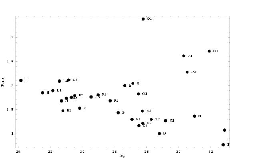
Figure 14: As Fig. 13 but for $P_{-1.5}$.

Figure 26: Line width parameter $b_{\sigma}$ against effective optical depth for various simulations after rescaling $\tau_{eff}$ and $b_{\sigma}$ to our standard model. We show the same simulations as in Fig. 9

Figure 36: The line shows the values of $\gamma_{912}$ and $\sigma_{8}$ that give simulated spectra that match observed $\bar{F}$ and $b_{\sigma}$. We increase the $X_{228}$ with increasing $\sigma_{8}$, as shown in Fig. 37.

Figure 37: As Fig. 36 but for $X_{228}$ and $\sigma_{8}$.

Figure 38: As Fig. 36 but for $X_{228}$ and $\gamma_{912}$.

References

- Abel et al. (1997) Abel, T., Anninos, P., Zhang, Y., & Norman, M. L. 1997, New Astronomy, 2, 181
- Abel & Haehnelt (1999) Abel, T. & Haehnelt, M. G. 1999, ApJ, 520, L13
- Anninos et al. (1997) Anninos, P., Zhang, Y., Abel, T., & Norman, M. L. 1997, New Astronomy, 2, 209
- Barkana & Loeb (2004) Barkana, R. & Loeb, A. 2004, ApJ, 609, 474
- Bolton et al. (2004) Bolton, J. S., Haehnelt, M. G., Viel, M., & Springel, V. 2004, MNRAS submitted (astro-ph/0411072)
- Bond et al. (1996) Bond, J. R., Kofman, L., & Pogosyan, D. 1996, Nature, 380, 603
- Bryan & Machacek (2000) Bryan, G. L. & Machacek, M. 2000, ApJ, 534, 57
- Bryan et al. (1999) Bryan, G. L., Machacek, M., Anninos, P., & Norman, M. L. 1999, ApJ, 517, 13
- Cen et al. (1994) Cen, R., Miralda-Escude, J., Ostriker, J. P., & Rauch, M. 1994, ApJ, 437, L9
- Croft (2003) Croft, R. A. C. 2003, astro-ph/0310890
- Croft et al. (2002) Croft, R. A. C., Weinberg, D. H., Bolte, M., Burles, S., Hernquist, L., Katz, N., Kirkman, D., & Tytler, D. 2002, ApJ, 581, 20
- Croft et al. (1998) Croft, R. A. C., Weinberg, D. H., Katz, N., & Hernquist, L. 1998, ApJ, 495, 44
- Eisenstein & Hu (1999) Eisenstein, D. J. & Hu, W. 1999, ApJ, 511, 5
- Freedman et al. (2001) Freedman, W. L., Madore, B. F., Gibson, B. K., Ferrarese, L., Kelson, D. D., Sakai, S., Mould, J. R., Kennicutt, R. C., Ford, H. C., Graham, J. A., Huchra, J. P., Hughes, S. M. G., Illingworth, G. D., Macri, L. M., & Stetson, P. B. 2001, ApJ, 553, 47
- Frigo & Johnson (1998) Frigo, M. & Johnson, S. G. 1998, in Proc. 1998 IEEE Intl. Conf. Acoustics Speech and Signal Proces sing, Vol. 3 (IEEE), 1381–1384
- Gardner et al. (2003) Gardner, J. P., Katz, N., Hernquist, L., & Weinberg, D. H. 2003, ApJ, 587, 1
- Gnedin & Hamilton (2002) Gnedin, N. Y. & Hamilton, A. J. S. 2002, MNRAS, 334, 107
- Haardt & Madau (1996) Haardt, F. & Madau, P. 1996, ApJ, 461, 20
- Hernquist et al. (1996) Hernquist, L., Katz, N., Weinberg, D. H., & Jordi, M. 1996, ApJ, 457, L51
- Hui & Gnedin (1997) Hui, L. & Gnedin, N. Y. 1997, MNRAS, 292, 27
- Hui & Gnedin (1999) Hui, L. & Gnedin, N. Y. 1999, in Evolution of Large Scale Structure, Garching, 1–13
- Hui et al. (2002) Hui, L., Haiman, Z., Zaldarriaga, M., & Alexander, T. 2002, ApJ, 564, 525
- Hui & Rutledge (1999) Hui, L. & Rutledge, R. E. 1999, ApJ, 517, 541
- Kim et al. (2001) Kim, T.-S., Cristiani, S., & D’Odorico, S. 2001, A&A, 373, 757
- Kim et al. (2004a) Kim, T.-S., Viel, M., Haehnelt, M. G., Carswell, B., & Cristiani, S. 2004a, MNRAS, 351, 1471
- Kim et al. (2004b) Kim, T.-S., Viel, M., Haehnelt, M. G., Carswell, R. F., & Cristiani, S. 2004b, MNRAS, 347, 355
- Kirkman et al. (2003) Kirkman, D., Tytler, D., Suzuki, N., O’Meara, J. M., & Lubin, D. 2003, ApJS, 149, 1
- Madau et al. (1999) Madau, P., Haardt, F., & Rees, M. J. 1999, ApJ, 514, 648
- Mandelbaum et al. (2003) Mandelbaum, R., McDonald, P., Seljak, U., & Cen, R. 2003, MNRAS, 344, 776
- McDonald (2003) McDonald, P. 2003, ApJ, 585, 34
- McDonald & Miralda-Escudé (2001) McDonald, P. & Miralda-Escudé, J. 2001, ApJ, 549, L11
- McDonald et al. (2000) McDonald, P., Miralda-Escudé, J., Rauch, M., Sargent, W. L. W., Barlow, T. A., Cen, R., & Ostriker, J. P. 2000, ApJ, 543, 1
- McDonald et al. (2004a) McDonald, P., Seljak, U., Burles, S., Schlegel, D. J., Weinberg, D. H., Shih, D., Schaye, J., Schneider, D. P., Brinkmann, J., Brunner, R. J., & Fukugita, M. 2004a, ApJsubmitted, astro-ph/0405013
- McDonald et al. (2004b) McDonald, P., Seljak, U., Cen, R., Bode, P., & Ostriker, J. P. 2004b, MNRASsubmitted, astro-ph/0407378
- McDonald et al. (2004c) McDonald, P., Seljak, U., Cen, R., Weinberg, D. H., Burles, S., Schneider, D. P., Schlegel, D. J., Bahcall, N. A., Briggs, J. W., Brinkmann, J., Fukugita, M., Ivezic, Z., Kent, S., & Berk, D. E. V. 2004c, ApJsubmitted, astro-ph/0407377
- Meiksin & White (2004) Meiksin, A. & White, M. 2004, MNRAS, eprint arXiv:astro-ph/0205387, 350, 1107
- Miralda-Escude et al. (1996) Miralda-Escude, J., Cen, R., Ostriker, J. P., & Rauch, M. 1996, ApJ, 471, 582
- Miralda-Escudé & Rees (1994) Miralda-Escudé, J. & Rees, M. 1994, MNRAS, 266, 343
- Rauch (1998) Rauch, M. 1998, ARA&A, 36, 267
- Rauch et al. (1997) Rauch, M., Miralda-Escude, J., Sargent, W. L. W., Barlow, T. A., Weinberg, D. H., Hernquist, L., Katz, N., Cen, R., & Ostriker, J. P. 1997, ApJ, 489, 7
- Sargent et al. (1980) Sargent, W., Young, P., Boksenberg, A., & Tytler, D. 1980, ApJS, 42, 41
- Schaye et al. (1999) Schaye, J., Theuns, T., Leonard, A., & Efstathiou, G. 1999, MNRAS, 310, 57
- Schaye et al. (2000) Schaye, J., Theuns, T., Rauch, M., Efstathiou, G., & Sargent, W. L. W. 2000, MNRAS, 318, 817
- Scott et al. (2000) Scott, J., Bechtold, J., Dobrzycki, A., & Kulkarni, V. P. 2000, ApJS, 130, 67
- Seljak et al. (2004) Seljak, U., Makarov, A., McDonald, P., Anderson, S., Bahcall, N., Brinkmann, J., Burles, S., Cen, R., Doi, M., Gunn, J., Ivezic, Z., Kent, S., Lupton, R., Munn, J., Nichol, R., Ostriker, J., Schlegel, D., Tegmark, M., Berk, D. V. d., Weinberg, D., & York, D. 2004, submitted to PRD, astro-ph/0407372
- Seljak et al. (2003) Seljak, U., McDonald, P., & Makarov, A. 2003, MNRAS, 342, L79
- Spergel et al. (2003) Spergel, D. N., Verde, L., Peiris, H. V., Komatsu, E., Nolta, M. R., Bennett, C. L., Halpern, M., Hinshaw, G., Jarosik, N., Kogut, A., Limon, M., Meyer, S. S., Page, L., Tucker, G. S., Weiland, J. L., Wollack, E., & Wright, E. L. 2003, ApJS, 148, 175
- Steidel et al. (2001) Steidel, C. C., Pettini, M., & Adelberger, K. L. 2001, ApJ, 546, 665
- Theuns et al. (1998) Theuns, T., Leonard, A., Efstathiou, G., Pearce, F. R., & Thomas, P. A. 1998, MNRAS, 301, 478
- Theuns et al. (2000) Theuns, T., Schaye, J., & Haehnelt, M. G. 2000, MNRAS, 315, 600
- Tormen & Bertschinger (1996) Tormen, G. & Bertschinger, E. 1996, ApJ, 472, 14
- Tytler et al. (2004) Tytler, D., Kirkman, D., O’Meara, J., Suzuki, N., Orin, A., Lubin, D., Paschos, P., Jena, T., Lin, W.-C., & Norman, M. 2004, ApJ, astro-ph/0403688, 617, 1
- Valageas et al. (2002) Valageas, P., Schaeffer, R., & Silk, J. 2002, A&A, 388, 741
- Viel et al. (2003) Viel, M., Branchini, E., Cen, R., Matarrese, S., Mazzotta, P., & Ostriker, J. P. 2003, MNRAS, 341, 792
- Viel et al. (2004a) Viel, M., Haehnelt, M., & Springel, V. 2004a, astro-ph/0404600
- Viel et al. (2004b) Viel, M., Weller, J., & M., H. 2004b, astro-ph/0407294
- Wadsley & Bond (1997) Wadsley, J. W. & Bond, J. R. 1997, in ASP Conf. Ser. 123: Computational Astrophysics; 12th Kingston Meeting on Theoretical Astrophysics, 332–+
- Zaldarriaga et al. (2001) Zaldarriaga, M., Hui, L., & Tegmark, M. 2001, ApJ, 557, 519
- Zhang et al. (1995) Zhang, Y., Anninos, P., & Norman, M. L. 1995, ApJ, 453, L57
- Zhang et al. (1997) Zhang, Y., Anninos, P., Norman, M. L., & Meiksin, A. 1997, ApJ, 485, 496
- Zhang et al. (1998) Zhang, Y., Meiksin, A., Anninos, P., & Norman, M. L. 1998, ApJ, 495, 63