Unveiling the Nature of the High Energy Source IGR J19140$+$0951

We report on high energy observations of IGR J19140$+$0951 performed with RXTE on three occasions in 2002, 2003 and 2004, and INTEGRAL during a very well sampled and unprecedented high energy coverage of this source from early-March to mid-May 2003. Our analysis shows that IGR J19140$+$0951 spends most of its time in a very low luminosity state, probably corresponding to the state observed with RXTE, and characterised by thermal Comptonisation. In some occasions we observe variations of the luminosity by a factor of about 10 during which the spectrum can show evidence for a thermal component, besides thermal Comptonisation by a hotter plasma than during the low luminosity state. The spectral parameters obtained from the spectral fits to the INTEGRAL and RXTE data strongly suggest that IGR J19140$+$0951 hosts a neutron star rather than a black hole. Very importantly, we observe variations of the absorption column density (with a value as high as $\sim 10^{23}$ cm^-2). Our spectral analysis also reveals a bright iron line detected with both RXTE/PCA and INTEGRAL/JEM-X, at different levels of luminosity. We discuss these results and the behaviour of IGR J19140$+$0951, and show, by comparison with other well known systems (Vela X-1, GX 301$-$2, 4U 2206+54), that IGR J19140$+$0951 is most probably a High Mass X-ray Binary.

1 Introduction

IGR J19140$+$0951 was serendipitously discovered during the first INTErnational Gamma-Ray Astrophysical Laboratory (INTEGRAL, Winkler et al. 2003) observation of the Galactic microquasar GRS 1915+105 (Hannikainen, Rodriguez & Pottschmidt 2003). Inspection of the high energy archives showed it to be the most likely hard X-ray counterpart of the poorly studied EXOSAT source EXO 1912+097 (Lu et al. 1996). Soon after its discovery a Target of Opportunity (ToO) was performed on IGR J19140$+$0951 with the Rossi X-ray Timing Explorer (RXTE). The preliminary spectral analysis of this ToO showed the source had a rather hard spectrum, fitted with a power law of photon index 1.6, and an absorption column density N_H=6$\times 10^{22}$ cm^-2 (Swank & Markwardt 2003). Recently timing analysis of the RXTE/ASM data revealed an X-ray period of 13.55 days (Corbet, Hannikainen & Remillard 2004). This analysis showed that the source was detected even during the early days of the RXTE mission, which suggests that IGR J19140$+$0951 is a persistent X-ray source although most of the time in a faint state. In a companion paper (Hannikainen et al. 2004a, hereafter Paper 1) we used the latest version of the INTEGRAL software to refine and give the most accurate X-ray position of IGR J19140$+$0951 (see also Cabanac et al. 2004), which allowed us to obtain the most accurate X-ray/Gamma-ray spectra of the source. High energy spectral analysis of IGR J19140$+$0951 covering the period of its discovery, i.e.. during INTEGRAL revolution 48, was presented for the first time. We have, in particular, shown, that during this observation, the source, although very variable, showed two distinct spectral behaviours. The first one manifests a thermal component (black body-like) in the soft X-rays, and a hard X-ray tail, whereas the second one is harder and can be interpreted as originating from thermal Comptonisation (Paper 1).
Although it is very likely that IGR J19140$+$0951 is a Galactic object, the nature of the compact object is unclear. The spectral analysis presented in Paper 1 would tend to favour a neutron star, but no definite conclusion could be drawn from the data presented.
We report here observations of IGR J19140$+$0951 with INTEGRAL performed between March and May 2003, during a very well sampled and unprecedented high energy coverage of this source. To our INTEGRAL monitoring, we add the analysis of the March 2003 RXTE ToO, as well as the analysis of observations performed one year earlier on EXO 1912+097, and the first RXTE observation of a monitoring campaign we are currently leading on IGR J19140+0951, performed in April 2004. We describe the sequence of observations and the data reduction procedures in Sec. 2, and then present the results obtained from the different instruments in Sec. 3. The results are discussed in the last part of the paper.

2 Observations and data reduction

The 1.2–12 keV RXTE/ASM, 20–40 keV and 40–80 keV INTEGRAL/ISGRI light curves of the source covering the period of interest are shown in Fig. 1.

Figure 1: top: One-day average 1.2–12 keV ASM light curve. We show here only the data covering the 2003 March–May period. middle & bottom: 20–40 keV and 40–80 keV ISGRI light curves over the same period. Note that the Crab luminosity corresponds to 75 cts/s for the ASM, and it is $\sim 114$ cts/s and $\sim 67$ cts/s for ISGRI, in the 20–40 and 40–80 keV ranges respectively.

2.1 INTEGRAL

The main instruments on board INTEGRAL are IBIS (Ubertini et al. 2003), and SPI (Vedrenne et al. 2003). Both instruments use coded masks which allow $\gamma$-ray imaging over large Fields of View (FOV), $\sim 30\times 30^{\circ}$ up to zero response. The Totally Coded FOV (TCFOV) is a smaller part within which the detector has the highest response. IBIS has a TCFOV of $9^{\circ}\times 9^{\circ}$, while that of SPI is 16^∘ (corner to corner). The INTEGRAL Soft Gamma-Ray Imager (ISGRI, Lebrun et al. 2003) is the top layer of the IBIS detection plane, and covers the energy range from 13 keV to a few hundred keV.
The JEM-X monitors (Lund et al. 2003), consist of two identical coded mask instruments designed for X-ray imaging in the range 3–35 keV with an angular resolution of 3 arcmin and a timing accuracy of 122 $\mu$s. The JEM-X FOV is smaller with a diameter of the fully-coded FOV of $4.8^{\circ}$. During our observation only the JEM-X unit 2 was being used.
We focus here on the monitoring of the source performed between its (re-)discovery by INTEGRAL, in March 2003 (Hannikainen et al. 2003) and May 2003, during which we obtained an unprecedented high energy coverage of the source. The journal of the INTEGRAL observations is presented in Table 1. Among the data acquired by our team with GRS 1915+105 as the main target (e.g. Hannikainen et al. 2004b), we obtained data through exchange with several other teams. Therefore, while in the former group of observations IGR J19140$+$0951 is always in the totally coded FOV of IBIS (and thus in the FOV of JEM-X), in the latter group of data the source lies in any position of IBIS, and is most of the time outside the JEM-X FOV. Note that in addition to those guest observer data, IGR J19140$+$0951 was observed during INTEGRAL Science Working Team ToOs on GRS 1915+105 (Fuchs et al. 2003). Those data are also included in this study. It should be noted that an INTEGRAL observation consists of a sequence of pointings (or science windows, hereafter SCW) following a certain pattern around the main target of the observation on the plane of the sky (Courvoisier et al. 2003). The patterns are also reported in Table 1. The chosen pattern has some importance on the amount of useful data. For an on-axis source (or close to as is IGR J19140$+$0951 in our revolutions), the hexagonal pattern allowed us to have the source always in the JEM-X FOV, while this is not so for the $5\times 5$ pattern. When the source is far off-axis, it may even be outside the FOV of IBIS in some SCW.

Table 1: Journal of the INTEGRAL observations presented in the paper. ^†(Mean) Angle between IGR J19140$+$0951 and the centre of the field of view. The total exposure represents the time spent by INTEGRAL on each field.

Rev. #	Start	Stop	Observing	Total Exposure	off-axis
	(MJD)	(MJD)	Pattern		angle†
48	52704.12	52705.37	Hexagonal	101 ks	1.1∘
49	52708.45	52709.16	5$\times$5	55 ks	9.3∘
51	52715.00	52715.66	5$\times$5	55 ks	9.3∘
53	52720.95	52721.62	5$\times$5	55 ks	9.3∘
56	52728.04	52728.79	5$\times$5	55 ks	9.3∘
57	52731 04	52732.29	5$\times$5	101 ks	1.1∘
58	52734.91	52735.62	5$\times$5	55 ks	9.3∘
59	52738.29	52739.41	Hexagonal	101 ks	1.1∘
60	52741.91	52742.62	5$\times$5	55 ks	9.3∘
62	52746 62	52747.91	5$\times$5	101 ks	1.1∘
67	52762.50	52763.54	5$\times$5	84 ks	4.9∘
68	52763.95	52766.45	5$\times$5	200 ks	4.9∘
69_1	52766.91	52768.37	5$\times$5	117 ks	4.9∘
69_2	52768.41	52769.5	Hexagonal	88 ks	1.1∘
70	52770.79	52772.08	5$\times$5	100 ks	4.9∘

Table 2: Level of systematic uncertainty applied to the spectral channels of the JEM-X spectra, and energy channel correspondence.

Channel	Energy	Systematic uncertainty
	(keV)	(%)
58–79	4.00–5.76	5
80–89	5.76–6.56	2
90–99	6.56–7.36	7
100–109	7.36–8.16	5
110–119	8.16–9.12	4
120–129	9.12–10.24	5
130–149	10.24–13.44	4
150–159	13.44–15.40	6
160–169	15.40–17.64	5
170–179	17.64–20.24	8
180–189	20.24–22.84	7
190–197	22.84–25.52	9

The JEM-X data were reduced using the Off-line Scientific Analysis (OSA) 4.1 software, following the standard procedure described in the JEM-X cookbook. Due to the faintness of IGR J19140$+$0951 we forced the source extraction at the position reported in Cabanac et al. (2004). We ran the analysis on all the revolutions considered here when IGR J19140$+$0951 was in the JEM-X FOV (48, 57, 59, 62, 67, 68, 69, 70) but only included the SCWs where the source was at an offset angle less than 5^∘. The level of systematic uncertainty applied to each spectral channel, and the energy-channel correspondence is reported in Table 2 (P. Kretschmar & S. Martínez Núñez priv. comm.). The IBIS/ISGRI data were reduced using version 4.1 of the OSA software. The data reduction procedure is identical to the one described in Paper 1, i.e. for each revolution we first ran the software up to the production of images and mosaics in the 20–40 and 40–80 keV energy ranges. The software was here free to find the most significant sources in the images. We then created a catalogue containing only the 9 brightest sources of the field (either detected in some of the revolutions or in all), and re-ran the software forcing the extraction of the count-rate of those sources. The data products obtained through the ISGRI pipeline therefore include 20–40 keV and 40–80 keV light curves (Fig. 1), with a time bin about 2200s (typical length of a SCW). Rather than using the standard spectral extraction, we extracted spectra from images/mosaics accumulated at different times. This non-standard method and its validity is described in Appendix 1.
First of all we restricted the spectral analysis to the times when the source was both in the IBIS and JEM-X FOV, i.e. revolutions 48, 57, 59, 62, 67, 68, 69 and 70. The distinction of the different times was defined from the 20–40 keV light curve (Fig. 1), on a SCW basis in a way similar to what is presented in Paper 1. The distinction of different times to accumulate the data from is solely based on the level of luminosity of the source during a SCW. Although the level on which the distinction is made is rather arbitrary, our approach allows us to try to understand the origin of the variability on the time scale of a SCW by accumulating spectra of similar (hard) luminosity. Although this approach can hide and completely miss the spectral variations on smaller time scales, it is dictated by the need to accumulate a large number of JEM-X and IBIS spectra to obtain good constraints on the spectral parameters (e.g. Paper 1). Our PCA analysis (Sec. 3.2) shows that although the source can be variable on short time scales, the fitting of the average spectrum leads to a rather good representation of the physics underlying the source emission. Here due to a larger sampling of the source as compared to Paper 1, it was possible to define more “states” to accumulate the spectra from, in order to understand better the origin of the variations and try to avoid possible mixture of different states together. We define here:

• The “ultra faint” state was accumulated from all SCW when the source had a 20–40 keV count rate (CR, measured in cts/s) $<$ 1.

• The “faint state” has a similar definition as in Paper 1 and was accumulated from all SCW where $1\leq\mathrm{CR}<3$.

• The “bright state” corresponds to $3\leq\mathrm{CR}<6$.

• The “ultra bright state” corresponds to the bright 20–40 keV flares, i.e. $\mathrm{CR}\geq 6$.

We caution the reader that these definition of “states” have nothing to do with the standard definition of spectral states usually employed in studies of X-ray Binaries (e.g. Tanaka & Shibazaki 1996), and that they refer to luminosity in the hard X-rays. We thus extracted the source count rate and error from 20 bin mosaics accumulated during these four intervals as described in Appendix 1. 6% systematics have been added to all spectral channels. The JEM-X individual spectra were averaged together following the same time distinction.
We also tentatively extracted SPI spectra following the standard method. However, the SPI angular resolution is about 2^∘, which renders the analysis of IGR J19140$+$0951 delicate given the proximity to GRS 1915+105, which is much brighter (Hannikainen et al. 2004b, Rodriguez et al. 2004a). In fact, an analysis of the SPI spectra showed that the parameters were consistent with those of GRS 1915+105. We therefore did not include the SPI data in our analysis.
The JEM-X & ISGRI spectra were then fitted in XSPEC v11.3.1, with latest rmf file for JEM-X (jmx2_rmf_grp_0021.fits), and the OSA 3.0 ISGRI matrices for IBIS (isgr_rmf_grp_0010.fits, isgr_arf_rsp_0004.fits). We retained the energy channels between 4 and 25 keV for JEM-X and those between 20 and 150 keV for ISGRI. Further rebinning of the JEM-X data was applied so that both ISGRI and JEM-X data give similar weight to the $\chi^{2}$ statistics in the spectral fittings.

2.2 RXTE data

The field of IGR J19140$+$0951 has been observed 3 times with RXTE during pointed observations, the journal of which is summarised in Table 3. Two observations were truly dedicated to IGR J19140+0951, a public ToO, and an observation that is part of an on-going monitoring programme of the source. The third and oldest observation was dedicated to EXO 1912+097. Whether or not IGR J19140$+$0951 and the EXOSAT source are the same is beyond the scope of this paper, given that the best position of IGR J19140$+$0951 (Cabanac et al. 2004) is still consistent with the EXOSAT position of EXO 1912+097 (Lu et al. 1996). We assume in the following that the sources are the same.
The RXTE data have been reduced with the LHEASOFT package v5.3.1, following the standard procedures for both Proportional Counter Array (PCA, Jahoda et al. 1996), and High Energy Timing Experiment (HEXTE, Rothschild et al. 1998) data. See e.g. Rodriguez et al. (2003a, 2004b) for the procedure of spectral extraction, and 2–40 keV (channel 5–92) high time resolution light curves. In addition, and since the source is quite weak, we further rejected times of high electron background in the PCA (i.e. times when the electron ratio in Proportional Counter Unit (PCU) $\#2$ is greater than 0.1), and time during the passage through the South Atlantic Anomaly (i.e. we retained the times since SAA$>30$ or $<0$ minutes) to define the “good time intervals”, and used the latest background files available for faint sources. The spectra were extracted from the top layer of all PCUs turned on during each observation. In order to account for uncertainties in the response matrix we added 0.8% systematics below 8 keV, and 0.4% above (Rodriguez et al. 2003a). Note that during the three observations, the data formats were different resulting in different time resolutions for the timing study. We could explore the source temporal behaviour up to 64 Hz, 4000 Hz, and 124 Hz in Obs. 1, 2, and 3 respectively. For HEXTE, we separated on and off source pointings and carefully checked for any background measurement pointing on GRS 1915+105, and other close-by sources (XTE J1908+094, X 1908+075, & 4U 1909+07). We only used the pointings which were not contaminated by other sources as background maps. However, due to either the weakness of IGR J19140$+$0951 or the limited number of background maps, no HEXTE data can sensibly be used in our analysis. We therefore focus on a comparison of the PCA spectra obtained during the 3 observations The spectra were fitted in XSPEC V11.3.1 (Arnaud 1996), between 3 and 25 keV.

Table 3: Journal of the RXTE observations discussed in the paper. ^† Net 3-25 keV mean count rate (cts/s)/PCU, only the top layers of PCUs are considered.

Obs. #	MJD	Exposure	# PCU	Count rate/PCU†
1	52394.08	3248 s	2	6.8
2	52708.79	2848 s	4	6.6
3	53087.50	6496 s	3	11.8

3 Results

3.1 High resolution temporal analysis

We studied the PCA high resolution light curves in different frequency ranges given the different time resolution of the different data format, in order to investigate the time variability and search for Quasi-Periodic Oscillations. We produce 2–40 keV Power Density Spectra (PDS) on an interval length of 16 s. Our PDS were normalised according to Leahy et al. (1983). The lower boundary of the PDS is 0.0625 Hz in each case while the higher boundary is 64 Hz, 4000 Hz, and 128 Hz for Obs. 1, 2 and 3 respectively. The 3 PDSs are well fitted with constants with best values 1.999$\pm 0.007$ ($\chi^{2}_{\nu}=1.10$ for 117 DOF), 2.002$\pm 0.001$ ($\chi^{2}_{\nu}=1.09$ for 199 DOF) and 2.004$\pm 0.004$ ($\chi^{2}_{\nu}=0.84$ for 139 DOF) (error at the 90% confidence level), compatible with the expected value for purely Poisson noise. In case a High Frequency QPO (HFQPO) is present it usually has a higher rms amplitude at energy higher than $\sim 5$–$7$ keV. We also produced a PDS in the 7–20 keV range from Obs. 2, and analysed it between 0.0625 Hz and 4000 Hz. A single constant fits the PDS well, with best value 2.000$\pm 0.001$ (at 90% confidence level), again indicative of purely Poisson noise.
Using

$$\mathrm{R}=\sqrt{2\times\mathrm{n_{\sigma}}\times\frac{\mathrm{S+B}}{\mathrm{S}^{2}}\sqrt{\frac{\Delta\nu}{\mathrm{T}}}}$$ (1)

where R is the fractional rms amplitude, S is the source net rate, B is the background rate, T and $\Delta\nu$ are the exposure time and the width of the QPO, one can estimate the 3$\sigma$ upper limit on the detection of any QPO at any frequency, during the 3 observations. The limiting amplitude being proportional to the square root of the width, the limit for a sharp QPO will be lower than that of a broad feature. The most constraining results are obtained for Obs. 3, for which the limit on the presence of a Q(=$\nu/\Delta\nu$)=10 low frequency feature is comprised between $1.5\%$ ($\nu=0.0625$ Hz) and 6.5% ($\nu=20.0$ Hz). This puts tight constraints on the presence of such a feature since those low frequency QPOs are usually observed to have a rather high fractional amplitude (e.g. 5–30%, McClintock & Remillard 2004). For high frequency QPOs, however, the situation is reversed. With the help of Equation 1, we obtain a limit of 17.4 % for a 200 Hz QPO during Obs. 2. This means that if such a feature was present (in the 100–300 Hz range for a black hole and in the kHz range for a neutron star) then we would miss it. This is even true for a $\sim 15\%$ rms HFQPO as sometimes detected in some Atoll sources (Swank 2004).

3.2 Spectral Analysis

Figure 2: INTEGRAL/JEM-X and ISGRI spectra with the best (physical) model superimposed in each case (see the text for details). The different component of the models (comptt, black body or Gaussian) are also plotted. From left to right, the panel correspond to the “Faint state”, the “Bright state”, the “Ultra bright state”. The vertical axis is in $\nu-F_{\nu}$ units. The lower panels represent the ratio between the model and the data in each of the ”states”.

Figure 3: RXTE/PCA spectra of EXO 1912+097/IGR J19140$+$0951 with the best fit model superimposed: a Gaussian at $\sim 6.5$ keV, plus an absorbed power law for the left and middle one, and an absorbed power law with a high energy cut-off for the right one. The spectra are time ordered from left to right (1 year separation). The Gaussian is represented in all 3 spectra. Note that the same vertical scale as that of Fig. 2 is employed to facilitate the comparison. The lower panels represent the ratio between the best model and the data.

3.2.1 Simultaneous JEM-X/ISGRI spectral analysis

Over a total of 450 SCW, covering revolutions 48, 57, 59, 62, 67, 68, 69 and 70, IGR J19140$+$0951 is found in the “ultra faint” state during 271 SCW (60.2%), it is in the “faint state” during 130 SCW ($\sim 28.9\%$), in the “bright state” during 37 SCW (8.2%), and in the “ultra bright” state during 12 SCW ($\sim 2.7\%$). However, due to the 5$\times$5 observing pattern (Courvoisier et al. 2003) and mean off axis angle during revolutions 67, 68, beginning of 69, and 70 (Table 1), the source is outside of the JEM-X FOV, during a large part of these revolutions. For the sake of consistency, we extracted mean spectra from the time when IGR J19140$+$0951 is in both the ISGRI and JEM-X FOV. However, in doing so some statistical sensitivity is lost especially at high energies, and we completely miss the flare occurring at the end of revolution 70 (Fig. 1). Finally, the selection based on the availability of JEM-X (good) data leads to effective exposures of $\sim 15$ ks, $\sim 55$ ks, $\sim 186$ ks, and $\sim 400$ ks for the “ultra bright”, “bright”, “faint”, and “ultra faint” states respectively. In all our spectral fits a constant was included to take into account the cross calibration uncertainties, and was found at a similar value.
Following the procedure presented in Paper 1, we first fitted the spectra from both instruments simultaneously, with a simple model consisting of an absorbed power law. The value of ${\mathrm{N}}_{\mathrm{H}}$, was frozen to the value obtained with RXTE (Swank & Markwardt 2003), i.e. $6\times 10^{22}$ cm^-2, since the useful energy range of JEM-X does not allow us to obtain a better constraint on this parameter. We note, however, that this parameter may change from one observation to the other (see our RXTE spectral analysis below), but the results of our 4–150 keV spectral analysis remain largely unchanged, this energy range being largely unaffected by absorption.
Since significant evolution at least in terms of luminosity, and possibly in terms of spectral parameters (Paper 1) is expected, we present here the results of the spectral fits to the different “states” separately.
“Ultra Faint State”: The source is not detected in any of the spectral channels of our ISGRI mosaic. Therefore it is not possible to construct a spectrum. We therefore did not include these data in our analysis since consistent comparison with the other states was not possible (mainly due to the lack of constraints on the possible hard tail, cut-off etc.)

“Faint State”: The simple power law model gives a poor fit to the data with a reduced chi square $\chi^{2}_{\nu}=2.56$ (47 DOF). Following the results from Paper 1, we added a black body component to the power law. This component is required at more than $5\sigma$. The best fit parameters are reported in Table 4. Replacing the power law by a cut-off power law (cutoffpl hereafter CPL) slightly improves the fit (the cut-off is required at just the $3\sigma$ level), but the cut-off energy is poorly constrained (E${}_{\mathrm{cut}}=44_{-18}^{+44}$ keV) (all along the text errors are given at the 90% confidence level). A good fit is also achieved with a simple power law and a Gaussian ($\chi^{2}_{\nu}=1.26$ for 44 DOF). The photon index is compatible ($\Gamma=2.32_{-0.08}^{+0.06}$) with the value obtained with the former model. The line parameters are those reported in Table 8. Note that the large uncertainty on the line parameters, its large width and normalisation could indicate a possible mixing of line and the black body emission, as will be discussed in Section 3.2.4. This possibility could explain well the inability of our fits to converge to sensible results when trying to fit the data including both the black body and the Gaussian.
We tentatively replaced the phenomenological models with more physical models of Comptonisation. Using the comptt model (Titarchuk 1994) alone does not provide a good fit to the data. As in the previous case, adding a black body component improves the fit significantly. The temperature of the seed photon for Comptonisation tends to too low values to be constrained. It is therefore frozen to 0.3 keV. The black body temperature is consistent with that obtained with the phenomenological model (kT=$1.42\pm 0.06$ keV). Note that if a Gaussian instead of the black body is added to the comptt, a good fit can be achieved, but the parameters of the line are not physically acceptable (the centroid tends to too low a value, while the width is too high). The JEM-X and ISGRI spectra are plotted with the comptt+bbody model superimposed in Fig. 2, left panel.

Table 4: Best fit parameters obtained for the “Faint state” observed with INTEGRAL. Errors are given at the 90% level. Fluxes are in units of erg cm^-2 s^-1

bbody+po	kT or kTe	$\Gamma$ or $\tau$	$\chi^{2}_{\nu}$	Unabs. flux
	(keV)		(DOF)	1-20 keV	20-200 keV
	1.51$\pm 0.07$	$2.35_{-0.08}^{+0.15}$	1.36 (45)	$2.24\times 10^{-9}$	$5.19\times 10^{-10}$
bbody+comptt	21${}_{-8}^{+1}$	1.3${}_{-1.0}^{+0.2}$	1.07 (44)	$1.83\times 10^{-9}$	$4.26\times 10^{-10}$

“Bright State”: Here again the simple model of an absorbed power law does not fit the data well ($\chi^{2}_{\nu}=2.78$ for 47 DOF). A cut-off component is not required at a high level ($\gtrsim 3\sigma$). A black body and a simple power law does not provide a good fit to the data. In fact, an alternative model of a power law with high energy cut-off and a Gaussian line provides a good fit to the data. The addition of the Gaussian leads to an improvement $\Delta\chi^{2}=36$ for $\Delta$DOF=3. The best fit parameters for this state are reported in Table 5, while the line parameters are discussed in Section 3.2.4. Note that besides the presence of the line, the spectral parameters are consistent with those presented in Paper 1.

Table 5: Best fit parameters obtained with the different spectral model for the “Bright”, and “Ultra Bright” states observed with INTEGRAL. Errors are given at the 90% level. Fluxes are in units of erg cm^-2 s^-1. Note that a Gaussian line is included in the fit in all models. CPL stands for cutoffpl in XSPEC terminology

State	model	$\Gamma$	Ecut or kTe	$\tau$	$\chi^{2}_{\nu}$	Unabs. flux
			(keV)		(DOF)	1-20 keV	20-200 keV
Bright	CPL	$2.05_{-0.14}^{+0.08}$	71${}_{-17}^{+29}$		1.48 (43)	$2.52\times 10^{-9}$	$7.32\times 10^{-10}$
	comptt		22.0${}_{-5.0}^{+15.6}$	$1.2_{-0.6}^{+0.5}$	1.44 (43)	$2.42\times 10^{-9}$	$7.12\times 10^{-10}$
Ultra Bright	CPL	$1.37_{-0.07}^{+0.14}$	$27.1_{-4.7}^{+6.7}$		1.49 (43)	$1.93\times 10^{-9}$	$9.54\times 10^{-10}$
	comptt		11.2${}_{-0.5}^{+0.8}$	$2.97_{-0.15}^{+0.36}$	1.75 (43)	$2.09\times 10^{-9}$	$1.03\times 10^{-9}$

Fitting the data with the comptt alone leads to $\chi^{2}_{\nu}=2.04$ for 45 DOF. Again a black body component is marginally detected ($\gtrsim 3\sigma$). As with the phenomenological model, the fit is greatly improved if a Gaussian instead of the black body is added to the comptt model. The Gaussian parameters are compatible with those found with the phenomenological model. Note that the temperature of the seed photon for Comptonisation is too low to be well constrained. We therefore fixed it at 0.3 keV. The best fit parameters are reported in Table 5, while the spectra are shown in Fig. 2 middle panel.

“Ultra Bright State”: As in the other “states” the single component model does not represent the data well ($\chi^{2}_{\nu}=3.61$ for 47 DOF). A high energy cut-off is required at more than $5\sigma$. Adding a black body does not bring significant improvement. On the other hand, adding a Gaussian improves the fit slightly ($\Delta\chi^{2}=15$ for $\Delta$DOF=3). The best fit parameters are reported in Table 5, while the line parameters are discussed in Section 3.2.4. Note that alternative models involving black body emission (either with a Gaussian and/or a high energy cut-off) do not provide a good description of the data. As in the “Bright” state the comptt provides an acceptable fit if a Gaussian is added to the model. The temperature of the seed photons for Comptonisation is again fixed at 0.3 keV. The line parameters are consistent with those found with the phenomenological model. The best fit parameters are reported in Table 5, while the broad band spectrum is shown in Fig. 2 right panel.

3.2.2 PCA spectral analysis

During the 3 RXTE observations the source was dimmer than when detected with INTEGRAL (see e.g. the differences between Fig. 2 and 3). We fitted the spectra with the same spectral models, first a simple absorbed power law, or simple absorbed black body or disc black body. While the latter models give a poor description of the data, the former (after addition of a Gaussian at $\sim 6.4$ keV to account for an excess due to Fe K complex emission) represents the data well for Obs. 1 and 2. The addition of the Gaussian leads to $\Delta\chi^{2}=56$, $\Delta\chi^{2}=101$ for $\Delta$DOF=3 in Obs. 1 and 2 respectively. The best fit parameters are reported in Table 6. The equivalent absorption column density ($N_{\mathrm{H}}$) was let free to vary in all spectral fits, and we note a slight decrease of $N_{\mathrm{H}}$ from Obs. 1 to Obs. 2 , the latter being consistent with the results reported by Swank & Markwardt (2003).
The simple power law+Gaussian model fails to represent Obs. 3 ($\chi^{2}_{\nu}=3.0$, 44 DOF). Replacing the power law by a CPL leads to a good fit, an F-test indicates the cut-off is required at more than 5$\sigma$. Note that the CPL alone does not provide a good fit to the data ($\chi^{2}_{\nu}=2.85$ for 46 DOF). The value of $N_{\mathrm{H}}$ is slightly lower than during Obs. 2 (Table 6). Because a cut-off power law is usually interpreted as a signature of thermal Comptonisation, we replaced the phenomenological model by the comptt model. This more physical model represents the data well, but we note, however, that due to the 3 keV lower boundary of the PCA spectra, the input photon temperature is very poorly constrained ($<1.12$ keV at 90%, if it is left as a free parameter). We then froze this parameter to 0.3 keV in a second run. The best parameters are reported in Table 6. We note here that the value of $N_{\mathrm{H}}$ is more consistent with that obtained during Obs. 2. The line parameters are discussed in Section 3.2.4.
We then re-performed the fits to Obs. 1 and 2, either adding a high energy cut-off (with highecut) or replacing the power law by a CPL. The improvement to the fits is only marginal (just at the $3\sigma$ level) for Obs. 1, and $\gtrsim 3\sigma$ for Obs. 2, therefore not at high significance. We also replaced the phenomenological models by comptt, and although a good fit is achieved the parameters (especially the electron temperatures) are found to be quite high and very poorly constrained. The three spectra and the best fit models (simple power law for the first two and CPL for Obs. 3) are plotted in Fig. 3, together with the ratio between the model and the data.

Since the model parameters (especially the power law photon index) are strongly correlated to the value of $N_{\mathrm{H}}$, we represent the error contours of the photon index $\Gamma$ vs. the value of $N_{\mathrm{H}}$, for the three observations in Fig. 4.
In addition to the simple power law fit, and in order to compare with the results from the fits to the INTEGRAL data, we tentatively fitted the spectra with the comptt model. The best fit parameters are reported in Table 6.

Figure 4: Error contours for the column density ($N_{\mathrm{H}}$) and the power law photon index ($\Gamma$) derived from the fits to the three RXTE/PCA spectra. The crosses mark the location of the best fit values, and the 68% and 90% confidence contours are shown.

Table 6: Best fit parameters obtained from the spectral fits to the RXTE/PCA data. The errors are reported at the 90% confidence level. PL stands for power law, CPL for cutoffpl in XSPEC terminology.

Obs. Number	model	$N_{\mathrm{H}}$	$\Gamma$	$\mathrm{E_{cut}}$ or kTe	$\tau$	unabs. 1-20 keV flux	$\chi^{2}_{\nu}$
		$\times 10^{22}$ cm-2		(keV) / (keV)	(keV) /	erg s-1 cm-2	(DOF)
1	PL	10.1$\pm 2.0$	1.64$\pm 0.11$			$1.60\times 10^{-10}$	0.95 (42)
2	PL	5.8${}_{-1.3}^{+1.4}$	1.74$\pm 0.08$			$1.47\times 10^{-10}$	0.99 (42)
3	CPL	3.85${}_{-1.5}^{+1.2}$	0.98${}_{-0.21}^{+0.17}$	13.7${}_{-2.6}^{+3.9}$		$2.37\times 10^{-10}$	0.95 (40)
	comptt	5.8${}_{-1.0}^{+0.9}$		5.0${}_{-0.4}^{+0.5}$	5.3${}_{-0.4}^{+0.5}$	$2.42\times 10^{-10}$	0.99 (43)

3.2.3 A closer look at RXTE observation 3

Since the 16 s PCA light curve shows that the source is very variable on short time scales, we separated the observation into two periods, one corresponding to the low and steady flux (second interval in Fig. 5 left), and the other one corresponding to the high flux and large variations (third interval in Fig. 5 left).
We applied the same (simple) models as discussed in the previous section. While for the first interval a simple absorbed power law (plus a Gaussian) fits the data well, the same model yields a poor fit for the second ($\chi^{2}_{\nu}$= 3.48 (44 DOF)). A cut-off improves the fit, and is required at more than 5$\sigma$. The best fit results are reported in Table 7, while the spectra and best fit models are shown in Fig. 5. In this case again the comptt fits the data well. The temperature of the seed photons is again fixed at 0.3 keV. As for the global spectrum, we remark that the absorption column returned from the fit with this model is slightly higher than the value obtained with CPL.

Table 7: Best fit parameters to the PCA fits of the two intervals from Obs. 3.

Interval	model	$N_{\mathrm{H}}$	$\Gamma$	$\mathrm{E_{cut}}$ or $kT_{\mathrm{e}}$	$\tau$	unabs. 1-20 keV flux	$\chi^{2}_{\nu}$
		$\times 10^{22}$ cm-2		(keV)		erg s-1 cm-2	(DOF)
1	PL	2.5${}_{-1.3}^{+1.0}$	1.86${}_{-0.10}^{+0.06}$			1.09$\times 10^{-10}$	0.87 (44)
2	CPL	5.4${}_{-1.2}^{+1.0}$	0.86${}_{-0.18}^{+0.15}$	11.9${}_{-1.8}^{+2.3}$		3.45$\times 10^{-10}$	0.83 (43)
	comptt	7.0${}_{-1.2}^{+1.0}$		4.7$\pm 0.3$	5.8${}_{-0.4}^{+0.6}$	3.84$\times 10^{-10}$	0.92 (43)

We note a significant evolution of the absorption column density and of the power law photon index between the two intervals. In order to check whether the evolution of both was real, we re-performed the fits freezing $N_{\mathrm{H}}$ to its mean value (Table 6). The spectral parameters obtained for both fits are compatible with those found leaving all parameters free to vary, except the power law photon index which tends to a softer value in interval 1 ($\Gamma=2.11\pm 0.05$), and a to harder one for interval 2 ($\Gamma=1.38\pm 0.03$). Since $N_{\mathrm{H}}$ and $\Gamma$ are tightly correlated, we also re-performed the fit freezing $\Gamma$ to its mean value, and allowing $N_{\mathrm{H}}$ to vary. While for interval 2 the spectral parameters obtained in this case are close to the ones obtained when everything is free to vary, this method yields a poor fit for interval 1. We take these results as evidence that both $\Gamma$ and $N_{\mathrm{H}}$ vary between both intervals. Note that this likely variation of the absorption is reinforced by the variations of $N_{\mathrm{H}}$ we observe between Obs. 1, 2 and 3 (Table 6).

Figure 5: TOP: 2-40 keV PCA (Top Layer of PCU 2) light curve of Obs. 3. MIDDLE & BOTTOM: Left: PCA 3-25 keV spectrum of interval 1, and its best fit model, the ratio between the model and the data is represented below. Right: Same as left but for interval 2. Note that the same vertical scale is employed in both to facilitate the comparison.

3.2.4 The iron line

As mentioned previously in all the INTEGRAL and RXTE spectra, an iron K$\alpha$ fluorescence line is required in the spectral fits. The parameters of the line obtained from the spectral fit to each observation are reported in Table 8. Note that these are obtained from the fits with the phenomenological models, but no significant differences are found in the spectra where a comptt model is used.

Table 8: Parameters of the iron line obtained from the spectral fits to the INTEGRAL and RXTE data. Obs. 1, 2, 3 refer to the average RXTE spectra, while Obs. 3 low and high refer to the sub interval presented in Section 3.2.3. Errors are given at the 90% confidence.

Obs.	Ecentroid	Width ($\sigma$)	Flux	Eq. width
	(keV)	(eV)	($\times 10^{-4}$  ph/cm2/s)	(eV)
Faint State	6.5${}_{-0.8}^{+0.4}$	1683${}_{-445}^{+587}$	$125_{-39}^{+81}$	$1560$
Bright State	7.2${}_{-1.3}^{+0.4}$	785${}_{-691}^{+1299}$	50${}_{-21}^{+112}$	535
Ultra Bright State	6.6$\pm 0.2$	$<475$	43${}_{-17}^{+19}$	410
Obs. 1	6.53$\pm 0.12$	$<518$	3.2${}_{-0.9}^{+1.1}$	385
Obs. 2	6.56$\pm 0.10$	375${}_{-363}^{+211}$	3.5${}_{-0.8}^{+0.9}$	469
Obs. 3	6.37${}_{-0.17}^{+0.13}$	419${}_{-181}^{+180}$	3.5${}_{-0.9}^{+1.6}$	258
Obs.3 low	6.44${}_{-0.15}^{+0.12}$	$<641$	2.1${}_{-0.6}^{+0.8}$	388
Obs.3 high	6.36${}_{-0.08}^{+0.13}$	460${}_{-296}^{+276}$	4.7${}_{-1.4}^{+2.2}$	213

One could wonder whether the line is intrinsic to IGR J19140$+$0951 itself, or whether it could originate from the Galactic background. The main argument that points towards an origin intrinsic to the system is that if the line was due to the Galactic ridge, we would expect its flux to be roughly constant. This is obviously not the case here.
It is interesting to note that in almost all cases, (except in the “Bright” and ”Faint” states), the parameters inferred for the line could be indicative of a narrow line, rather than a broad line. In fact for both instruments the upper limit on the line width indicates that we are limited by the instrumental spectral resolution. The case of the faint and bright states seem different since our fits indicate a broad line (Table 8). Our spectral fits to the INTEGRAL data (Sec. 3.2.1) indicate that the “Bright” state is spectrally intermediate between the “Faint” state and the “Ultra-bright” one, as we will discuss further below. In particular in the soft X-rays (4–8 keV), a black body component could be present in the spectra of the “Bright” state, and represents the data well for the faint state. In both cases, a fit to the data with a black body and a Gaussian (besides the power law) does not converge on sensitive parameters for either of the components. The broad line we found instead could be indicative of a “mixture” of faint black body emission (poorly constrained given the 4 keV lower boundary of our fits) and a Gaussian line. This possibility is compatible with the evolution between the three INTEGRAL “states”, as clearly seen of Fig. 2, where black body emission dominates the soft X-ray in the “Faint state” (when either no line is needed or a very broad one), to the “Ultra Bright” state, where no black body is detected, and with a good constraint on the line.

4 Discussion

4.1 A neutron star primary?

We performed a thorough spectral analysis of the INTEGRAL source IGR J19140$+$0951 using a well-sampled high energy monitoring with INTEGRAL in 2003 March–May, and adding 3 RXTE observations performed at different epochs. As already observed (Paper 1), IGR J19140$+$0951 is highly variable on timescales from months down to hours, and it can show variations on shorter timescales as seen during RXTE observation 3 (Fig. 5). This behaviour is reminiscent of Galactic X-ray binaries (XRB), and our deep analysis further confirms the Galactic nature of IGR J19140+0951, already proposed in other publications (Paper1, Corbet et al. 2004).
When observed with RXTE, the source was dim, with a 1-200 keV (unabsorbed) luminosity of $\sim 3.4\times 10^{36}\times$(D/10 kpc)² erg/s (Obs.3), and a spectrum typical of Comptonisation of soft photons by a low temperature plasma ($kT\sim 5$ keV) with a relatively high optical depth ($\tau\sim 5$). This could correspond to the “ultra faint state” which seems to be the state in which the source spends most of its time as indicated by our INTEGRAL monitoring. During the INTEGRAL observations, the luminosity is up to about 10 times higher, with a maximum of $\sim 3.7\times 10^{37}\times$(D/10 kpc)² erg/s. Here significant spectral evolution is observed since in one case a bright thermal component may be present in the soft X-rays while it is either marginal or not detected in the other “states” defined from the ISGRI light curve. A clear pivoting between the three INTEGRAL spectra is clearly visible (Fig. 2). The phenomenological models may indicate a spectral transition from something resembling a standard soft state to a hard state (Tanaka & Shibazaki 1996), as seen in BHC, but the temperature of the black body, and the parameters of the Comptonisation, especially during the faint RXTE observations are more comparable to those of a neutron star primary. The spectral parameters obtained from our fits during the “Bright state” indicate that it is spectrally intermediate between the “Faint” state and the “Ultra bright” state (Tables 4 and 5). A hint for a black body component is indeed found here, although the best fit involves an iron line. The large width of the latter, and the inability of our fits to converge when trying to model the spectra with both the line and the black body, tend to indicate that the huge line is in fact a mixture of a narrower feature with a fainter and cooler thermal component, for which no constraints can be obtained with the 4 keV lower boundary of our spectral analysis.
In order to try to constrain the primary type, we first compare the source luminosity with that of other known Galactic XRBs. To do so we plotted the 20-200 keV vs 1-20 keV luminosities for the brightest INTEGRAL and RXTE states, at three different distances and over-plotted it with those presented in Barret et al. (1996) (Fig. 6).

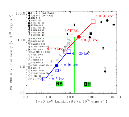
Figure 6: IGR J19140$+$0951 luminosities as obtained from the spectral fits presented in this paper, and comparison with the “classification” proposed in Barret et al. (1996). The two continuous lines ending with squares indicate the positions of IGR J19140$+$0951 as obtained in this study with INTEGRAL and RXTE assuming three different distances (open squares are at 5 and 20 kpc, filled circles are at 10 kpc) for IGR J19140+0951. Based on Barret et al. (1996), systems with neutron star primaries would rather lie in the bottom left corner (“X-ray burster box”) of the plot, whereas system with black hole binaries would lie outside this box (see however di Salvo et al. 2001).

It is clear from Fig. 6 that, unless the source is at a large distance of 20 kpc or beyond, it always falls in the “X-ray burster box”, except for the INTEGRAL point at 10 kpc, which is exactly half way between the 2 standard states of Cyg X-1. However the delimitation between the two regions is purely empirical and based on measurements made up to 1996, on a sample of X-ray bursters only for the neutron stars (which at the time of writing were the only known neutron star X-ray binaries with hard X-ray tails extending to at least 100 keV). Since then, Di Salvo et al. (2001) have indeed shown that some neutron star systems, could definitely lie outside this so called “X-ray burster box”. Therefore unless a very high luminosity hard tail is found, the fact that a source lies outside the “X-ray burster box” is not a definite proof for a black hole binary (Di Salvo et al. 2001). In addition, the spectral parameters we obtain from our spectral fits in all “states” are radically different from those usually observed in black hole binaries (e.g. McClintock & Remillard 2004), even in their quiescent states (e.g. Kong et al. 2002). This is particularly true for the parameters of the cut-off energy, or equivalently the electron temperature which are in agreement with those presented by Barret (2000) in the case of neutron star primaries.
As already pointed out in another system (4U 2206+54 Torrejón et al. 2004), we note that during the “Faint” state the black body temperature is high, while the source luminosity is not very high (although higher than in 4U 2206+054). Following the procedure presented by Torrejón et al. (2004), we can estimate the radius of the black body emitter following $R_{bb}=3\times 10^{4}\times{\mathrm{d_{kpc}}}\sqrt{f^{\mathrm{bol}}/(1+y)}/{\mathrm{kT_{bb}}}$ (in’t Zand et al. 1999), where y is the Compton parameter $y\propto\mathrm{kT_{e}\tau^{2}}$, $f^{bol}$ the “bolometric” flux and kT_bb the black body temperature. Using the values found in our study (expanding the flux to the 0.1-200 keV range following in’t Zand et al. 1999), we obtain R_bb=0.999$\times\mathrm{d_{kpc}}$ km. We remark here a factor of 2 discrepancy between Torrejón et al. (2004) and in’t Zand et al. (1999), the values given in the former are the diameter of the black body emitter, but this does not change their conclusions. This value implies that even at a very far distance (e.g. 20 kpc, therefore outside of our Galaxy, which appears rather unlikely), the black body radius is consistent with the radius of a neutron star.

4.2 Possible type of the system

The absorption column density ($N_{\mathrm{H}}$=$\sim 3$–$10\times 10^{22}$ cm^-2) of IGR J19140$+$0951 derived from the spectral fits to the RXTE data is much higher than the Galactic absorption towards the source (1.26$\times 10^{22}$ cm^-2 Dickey & Lockman, 1990). This favours an absorption intrinsic to the object, and therefore the presence of absorbing material in the vicinity of the compact object. The variations of the absorption (Fig. 4 and Table 7) also point toward an absorption intrinsic to the source. This is in fact similar to what is observed in IGR J16320-4751 (Rodriguez et al. 2003b), or 4U 1700$-$37 (Boroson et al. 2003), in which the absorption is seen to vary by a factor of about 2 in the former source (a most likely High Mass X-ray Binary HMXB; Rodriguez et al. 2003b) and 10 in the latter (a dynamically confirmed HMXB). The presence of absorbing material is consistent with the detection of a (cold) iron line. It is interesting to note that although when comparing Obs. 1, 2 and 3, the iron line fluxes are all comparable within the uncertainties (Table 8), while $N_{\mathrm{H}}$ varies significantly, the line flux is much stronger in Obs. 3 high (interval 2), than in Obs. 3 low (interval 1), i.e. it is stronger here when $N_{\mathrm{H}}$ is higher. In addition, there seems to be a tight correlation between the 1-200 keV (unabs.) flux of IGR J19140$+$0951 and the flux of the line although the case of the “Faint” state does not obey this relation, and the parameters of the line are poorly constrained in the “Bright” state. This relation, and the relative constancy of the line energy in most of the cases suggest that the line is produced through fluorescence in a cold medium as in e.g. Vela X-1 (Ohashi et al. 1984). In addition, the intensity of the iron line during the INTEGRAL observations is comparable to the intensity observed in the HMXB GX 301$-$2 at a similar flux (Saraswat et al. 1996). In the latter system the line width (measured with ASCA) was consistent with the instrumental spectral resolution, which seems to be the case in IGR J19140+0951, although the energy resolution of both RXTE/PCA and INTEGRAL/JEM-X is very poor in comparison to that of ASCA/SIS. These similarities between different systems would tend to indicate IGR J19140$+$0951 is an HMXB, rather than a system containing a low-mass secondary star (LMXB). Finally we observe that the hardest spectra (i.e. those for which the electron temperature or the cut-off energy is the highest) are observed at higher luminosities, which again is very similar to the HMXB 4U 2206+54 (Masetti et al. 2004), and rather contrary to what observed in the case of LMXB (Barret 2001).
Independently, the temporal variability on timescale $\sim$1000 s is very similar to the HMXBs 4U 2206+054 (Nereguela & Reig 2001), 2S 0114+65 (Yamauchi et al. 1990), and Vela X-1 (Kreykenbohm et al. 1999). In these systems, this variability is commonly interpreted as due to random inhomogeneities in the accretion flow (e.g. Masetti et al. 2004 and references therein). The level of variability from 0.06 Hz on is compatible with what was found in 4U 1700-37 (Boroson et al. 2003) or 4U 2206+54 (Nereguela & Reig 2001), i.e. the variability is compatible with purely Poisson noise. In the former source significant aperiodic variability is detected only below 0.01 Hz, although a 13 mHz QPO is detected at a fractional amplitude 4.0 % (Boroson et al. 2003). As discussed in Sec. 3.1, if such a feature was present in IGR J19140+0951, it should have been detected at least in RXTE Obs. 3. In 4U 2206+54, on the other hand, significant aperiodic variability is seen below $\sim 0.06$ Hz. However, no QPOs are detected in this system. Again the similarity of the behaviour of IGR J19140$+$0951 with that of confirmed HMXB, would tend to argue in favour of a high mass secondary star in IGR J19140$+$0951 and therefore X-ray luminosity due to wind accretion onto the compact object.
The hypothesis of IGR J19140$+$0951 being a HMXB is again in good agreement with the relatively large value of the orbital period of 13.55 days (Corbet et al. 2004), since HMXBs have usually higher orbital period than LMXBs. Note that this is not a definite proof since some LMXB can have large orbital period as e.g. GRS 1915+105 and GRO J1744-28 with $\sim 33$ days and $\sim 12$ days, respectively. The fact that the modulation is sinusoidal (Corbet et al. 2004) would tend to indicate a high inclination system (i.e. the orbital plane almost parallel to the line of sight) rather than variations of the X-ray flux due to perigee passage of the compact object in a highly eccentric orbit.
Finally, it should be noted that IGR J19140$+$0951 lies in the direction of the Sagittarius arm of our Galaxy, which is a region rich of high mass/young stars, and therefore HMXBs. This location could provide another indirect support for IGR J19140$+$0951 being a HMXB, as proposed for 3 similar sources lying in the Norma arm (Revnivtsev 2003). This arm is located about 2 kpc from the Sun, and if IGR J19140$+$0951 was associated with this region its luminosity as obtained from our spectral fit (10³⁵-10³⁶ erg s^-1) would be completely consistent with that of the aforementioned HMXB/neutron star binaries, as Vela X-1.

5 Conclusion

We have presented a detailed study of the hard X-ray properties of IGR J19140$+$0951 observed at different times with INTEGRAL and RXTE. From a well-sampled monitoring of the source in 2003 March–May, we deduced that IGR J19140$+$0951 spends most of its time in a low luminosity state, which likely corresponds to the state observed with RXTE on three occasions. The source spectrum is characteristic for thermal Comptonisation, and on one occasion we have evidence for a black body component in the spectrum. From the comparison of the spectral properties of IGR J19140$+$0951 with those of other XRBs, we suggest that this system hosts a neutron star rather than a black hole.
The source spectra show evidence for a variable intrinsic absorption which indicate that the compact source is embedded in a dense cloud. This and the detection in all our spectra of a bright (and thin) iron line, whose flux is higher in the higher luminosity states points towards radial accretion from a stellar wind. Therefore it is very likely that IGR J19140$+$0951 is a HMXB, with properties similar to those of other well known HMXB.
The arguments presented in the present study are, however, only indicative, none of them being definite. In particular the identification of counterparts at other wavelengths of the electromagnetic spectrum should allow one to truly confirm the nature of the system and/or the compact object. Such a study is, however, not possible at the moment given the relatively large error on the position of the source. Observations with high resolution X-ray satellites, such as Chandra or XMM-Newton, should permit a better position to be found, counterparts to be searched for, and possibly determine whether IGR J19140$+$0951 is indeed the same source as EXO 1912+097. In addition such a study should permit one to obtain much better constraints on the absorption and line parameters.

Appendix 1: ISGRI Spectral extraction from images

Principle of the method

Numerous issues with OSA, which remains under development, are reported on the ISDC website’ Of particular relevance to this work : “ii_spectra_extract runs per science window and in case of weak sources, addition of many spectra obtained for the different science windows may give a bad total spectrum. Spectral reconstruction is very sensitive to the background correction. In certain cases running the imaging procedure on several (large) energy bands can provide a better spectrum” .
We therefore extracted the spectra of IGR J19140+0951 using a method based on the count rates extracted from the images. For the whole data set (only restricted to the SCW where the source is less than 5^∘ from the center of the FOV), we ran the software up to the IMA level. We extracted the products 20 energy bins defined such that they match exactly the boundaries of the redistribution matrix file (rmf). The energy bands are 20.65-24.48, 24.48-28.31, 28.31-32.14, 32.14-35.97, 35.97-39.8, 39.8-43.36, 43.36-49.38, 49.38-53.21, 53.21-57.04, 57.04-60.87, 60.87-68.52, 68.52-76.18, 76.18-87.67, 87.67-99.16, 99.16-122.14, 122.14-150.86, 150.86-196.82, 196.82-300.22, 300.22-518.5, 518.5-1000 keV. Note that the energy ranges above $\sim 300$ keV are of limited use for most of the sources.
Once this is finished, for each SCW, the intensity, exposure, variance and significance maps of the field are obtained in each of the aforementioned energy ranges. The average count rate, $F(E_{i},\alpha,\delta)$, in the energy range $E_{i}$, over a list of $p$ SCW, at the position ($\alpha$, $\delta$) of a given source is given by:

$$F(E_{i},\alpha,\delta)=\frac{\sum_{j=1}^{p}\frac{F_{j}(E_{i},\alpha,\delta)}{var_{j}(E_{i},\alpha,\delta)}}{\sum_{j=1}^{p}\frac{1}{{var_{j}(E_{i},\alpha,\delta)}}}$$ (2)

where $F_{j}(E_{i},\alpha,\delta)$ is the count rate in SCW #j, in the energy range $E_{i}$ at a (sky) position ($\alpha$, $\delta$), and $var_{j}(E_{i},\alpha,\delta)$ is the associated variance value.
Repeating Eq. 2 from i=1, to i=20 (in our case) allowed us to obtain the source spectrum over the given list of SCW.

Validity of the method: estimate of a Crab spectrum

In order to validate our method, we extracted a Crab spectrum following the same method. In order to be even more rigourous, we restricted our comparison to Crab observations performed with the same observing pattern as most of our observations, i.e. a hexagonal pattern. However we point out that a check on an arbitrary pattern gave similar and consistent results. The validation of the spectral extraction method is currently a work in progress and detailed results and issues will be presented in a forthcoming paper (Lubinski et al. in prep.). In general, and for what concerns this work, the discrepancy between the standard spectral extraction and this new method does not exceed 5% (Lubinski private comm.). Our particular spectral analysis of the Crab using both methods showed that the spectral parameters were compatible within 1% for the photon index, within about 5 % for the normalization, and the 20-200 keV flux discrepancy is about 2%.