An Alternate Estimate of the Mass of Dust in Cassiopeia A

Recent observations of sub-millimeter continuum emission toward supernova remnants (SNR) have raised the question of whether such emission is caused by dust within the SNR itself or along the line-of-sight. Here we make a comparison of the image of sub-mm emission from dust with the integrated $J=1-0$ line emission from interstellar ¹³CO  toward the SNR Cassiopeia A based on existing data. The cm and mm synchrotron emission from Cas A has a rather symmetric, ring-like structure whereas both the sub-mm continuum and interstellar ¹³CO  line emission are located mostly toward the south of the SNR. There is positional agreement for 3 of 6 maxima found in ¹³CO  line and sub-mm continuum emission, with the weakest feature near the center of Cas A and the other two features near the southeast and west edges of the SNR. For these three maxima, a comparison of masses determined from dust and ¹³CO  data shows good agreement if we use the 450 $\mu$m dust absorption coefficient typical for diffuse clouds. There is also good agreement between the sub-mm dust temperature and the gas kinetic temperature from CO and NH₃. For the remaining sub-mm continuum peaks, one is outside the forward shock of the SNR. For the other two, one was not mapped in ¹³CO; for the other there is no ¹³CO emission. Hi  absorption covers all of Cas A, but the Hi  column density may be too small to account for the sub-mm dust emission. Thus it is possible that one, or perhaps two of these sub-mm continuum peaks are located inside the SNR. From lower resolution maps in CO lines, the SE and W features are the edges of extended clouds. Toward the cloud centers, the CO emission is more intense, but there appears to be less sub-mm dust emission. The differences between CO and sub-mm images may be caused a combination of the techniques used to produce the sub-mm maps and changes in cloud properties from center to edge.

1 Introduction

Large amounts of dust have been observed in a number of galaxies with large redshifts (see e.g. Smail et al. sma (1997), Eales et al. eal (2003)). Dust is produced in red giant stars and ejected in winds, but Morgan and Edmunds (mo2 (2003)) argue that this process is too slow to explain the presence of large amounts of dust in the early universe unless the star formation rates are very large. Morgan et al. (mo1 (2003)) have presented an image of dust emission of Kepler s supernova remnant (SNR) and estimate that 1 M_⊙ of dust is produced. Dunne et al. (dun (2003)) have estimated that Cassiopeia A has produced 2 to 4 M_⊙ of dust. On the basis of this data and the data of Morgan et al. (mo1 (2003)), Dunne et al. (dun (2003)) have argued that large amounts of dust can be produced in SNe. In the Cas A image, much of the dust emission is concentrated toward the southern part of the SNR. Dunne et al. (dun (2003)) had assumed that all of the dust which gives rise to sub-mm emission is contained in the SNR itself and was produced by the SNR itself. From a comparison of 24 $\mu$m, 70 $\mu$m and sub-mm dust images, Hines et al. (2004) noted that if the dust emitting at sub-mm wavelengths resides within the SNR, it must have very different properties from the dust emitting in the mid-IR. Batrla et al. (bat (1984)), Troland et al. (1985), Wilson et al. (1993), Gaume et al. (1994) and Liszt & Lucas (1999) have measured molecular absorption and emission toward the southern part of Cas A. These results give a gas kinetic temperature which is the same as the temperature reported by Dunne et al. (dun (2003)). In fact all of these temperatures are about the same as the equilibrium temperature of cirrus clouds deduced from COBE satellite data (Lagache et al. 1998). Thus, at least some of the sub-mm dust emission assigned to the SNR by Dunne et al. (dun (2003)) may arise in the interstellar medium (ISM).

In this paper, we compare the spatial distribution of sub-mm dust emission (15^′′ resolution) with ¹³CO  emission (21^′′ resolution), CO emission (28^′′ resolution), with Hi  absorption (7^′′ resolution) toward Cas A, and with CO maps (2.5’ resolution) around Cas A to separate sub-mm dust emission from interstellar clouds toward the SNR Cas A from sub-mm dust emission arising from within this SNR.

2 Comparison of Results

2.1 Qualitative Comparison

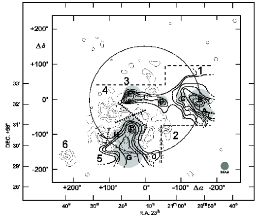
Figure 1: Overlay of the $J=1-0$ ¹³CO  integrated line intensity, shown as thick contours, starting at 4 K km s^-1, in steps of 2 K km s^-1 to 18 K km s^-1 (from Wilson et al. (wil (1993))) on 450 $\mu$m sub-mm dust emission image, shown as thin contours (from Dunne et al. (dun (2003))). The B1950.0 coordinates are taken from Wilson et al. (1993). See Fig. 2 for a map of a larger region in the CO $J=2-1$ line. We have numbered the sub-mm dust emission maxima 1 to 6. The ¹³CO  clouds are labeled with capital letters A to H. Shaded circles show the FWHP and location of ¹³CO  clouds (from Wilson et al. (wil (1993))). The sub-mm dust peaks under E and F do not have higher contours for clarity. The thick dotted lines mark the boundaries where we have divided the sub-mm dust emission between peaks 2, 3, 4, and 5. We used these as the boundaries of integrations to determine the masses of individual regions.

The ¹³CO  J=1–0 line data for our comparison were taken with the IRAM 30-m radio telescope on Pico Veleta. The angular resolution was 21^′′, the observing method position switching with the reference position 60’ north of the center of Cas A. The most important point is that all of the ¹³CO  emission, even from very extended clouds, was recorded. Details are to be found in Wilson et al. (wil (1993)).

The sub-mm data presented by Dunne et al. (dun (2003)) were taken with a 15^′′ angular resolution. Observational details are given by Loinard et al. (2003). To suppress atmospheric emission, one should difference the signal between two regions of the sky separated by a number of beamwidths; images made from this data were restored using the procedures described by Johnstone et al. (john (2000)). Johnstone et al. (john (2000)) present a number of data reduction techniques; that used by Dunne et al. (dun (2003)) is from Emerson et al. (1979 hereafter EKH). All restorations tend to suppress the signal from structures with sizes larger than twice the maximum chopper throw, and also increases the noise in the corresponding Fourier components. According to Johnstone et al. (2000), the EKH method produces lower quality images near map edges. Loinard et al. (2003) did not specify their chopper throw, but the maximum throw used at JCMT is 120^′′. The restoration process produces sub-mm emission maps at 850 and 450 $\mu$m. A map of the synchrotron emission (see e.g., Wright et al. 1999), scaled in frequency, was subtracted from these images. The final 450 $\mu$m image is given in Fig. 4 of Dunne et al. (dun (2003)). Although the error beam of the telescope is larger at 450 $\mu$m and atmospheric quality is worse than at 850$\mu$m, the sub-mm dust intensity is larger, so the sub-mm dust emission is less affected by possible residual synchrotron emission from the SNR. All our comparisons are made with the 450 $\mu$m map.

In Fig. 1 we show an overlay of the J=1–0 ¹³CO  integrated line intensity image (Fig. 3 of Wilson et al. wil (1993)), shown as thick contours with the 450 $\mu$m dust image (Fig. 4 of Dunne et al. dun (2003)) shown as thin contours. The ¹³CO  clouds are labelled using capital letters taken from Wilson et al. (wil (1993)). Shaded circles show the gaussian Full Width to Half Power (FWHP) sizes and locations of ¹³CO  clouds, as cataloged by Wilson et al. (wil (1993)). The thin circle of radius 153^′′, centered on offset ($\Delta\alpha,\Delta\delta$=0^′′, 0^′′) marks the location of the forward shock from the SNR. The dust is thought to form inside this shock, but sub-mm dust peak 6 (at (216^′′, -163^′′)) clearly lies outside. The shaded circle at the right bottom is the half power beam width for the ¹³CO  data, 21^′′. The box containing the offset coordinates is the full size of Fig. 4 of Dunne et al. (dun (2003)). The dashed lines show the limits of the region in which the ¹³CO  $J=1-0$ line was fully sampled.

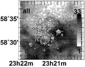
Figure 2: Adapted from Liszt & Lucas 1999; the coordinates are B1950.0. The gray scale is the $J=2-1$ CO emission toward Cas A, summed from V=-30 to -50 km s^-1. The wedge on the right side of the image, with numbers from 1 to 33, is the scale for integrated intensity in units of K$\cdot$km s^-1. The white crosses indicate where spectra were taken with longer integrations by Liszt & Lucas (1999). The range of radial velocity is basically the same as that used to form the ¹³CO  image, shown as thick contours in Fig. 1. The angular resolution of the CO data is 28^′′. The black contours are the 140 GHz continuum from the SNR Cas A measured by Liszt & Lucas 1999, with angular resolution 44^′′. This is dominated by synchrotron emission. We have superposed the sub-mm dust emission contours from Fig. 4 of Dunne et al. (dun (2003)) as white contours. This image shows that most of the CO is located south of Cas A, as is the sub-mm dust emission. The ¹³CO  extent (Fig. 1) is smaller than that of the CO because of lower optical depth.

To show the full extent of CO emission toward Cas A, in Fig. 2, we show the gray scale image of the $J=2-1$ line of CO superposed on contours of the continuum emission from Cas A at 140 GHz (Liszt & Lucas 1999). This 28^′′ resolution image shows more intense CO emission to the SE and SW of the center of Cas A, but little to the north. The optical depth of the CO lines is $>$5 (Troland et al. (1985), but the isotopic ratio of CO/¹³CO  for these clouds is 1/60 (Wilson & Rood 1994), so the ¹³CO  lines are optically thin, and so the ¹³CO  line emission traces H₂ column density. In addition, the intensity of the ¹³CO  line emission is always small and the ¹³CO  emission always has a smaller extent than CO emission (see e.g., Section 14.8.1 in Rohlfs & Wilson 2003). Thus even though the ¹³CO  data in Fig 1 (between the dashed lines) does not cover the northern part of Cas A, one can be certain that there is no ¹³CO  emission from this region. In Fig. 3, we show the lower resolution CO $J=1-0$ line maps of Troland et al. (1985). There is emission over a wide region to the south of Cas A. We have added a thick square box to the figure of Troland et al. (1985) to show the maximum area mapped by Dunne et al. (2003) at 850 $\mu$m. The region in Fig. 1 is 20% smaller. From the ¹³CO  and CO data, it is clear that the CO emission measured toward Cas A arises from the edges of larger clouds. These clouds have small peak temperatures, so are low density interstellar clouds that contain no embedded high mass stars. From these data it is evident that:

(1) there is sub-mm dust emission to the south of Cas A, but not toward the northern part of Cas A.

(2) The synchrotron radio continuum emission from Cas A is highly symmetric (Fig. 2 and Wright et al. 1999).

(3) Most of the molecular clouds are found toward the south of Cas A.

(4) There is a least one sub-mm dust emission peak, clump 6, outside the forward shock of the SNR. This cannot be a projection effect, but the location of clump 3 might be.

There is spatial overlap of three sub-mm dust maxima of Dunne et al. (2003) with groups of ¹³CO  peaks toward the SE of the SNR (clouds F, G, and H), toward the center (cloud E), and toward the west(clouds A, B and C). There is very little CO or sub-mm dust emission toward the north of Cas A. This leads one to suspect a possible connection between the CO clouds in the ISM and the sub-mm dust emission measured by Dunne et al. (2003). From Fig. 1 the sub-mm dust emission decreases outside the forward shock. Assuming that the sensitivity and response of the sub-mm dust measurements of the region shown as a box in Fig. 3 are uniform, and if there is a proportionality between CO, ¹³CO  and sub-mm dust emission in interstellar clouds, we must explain the decrease in sub-mm dust emission to the south of Cas A. There are two possible causes:

(1) A change in cloud properties from the edge to cloud center. As is widely accepted, molecular clouds consist of many small clumps (see e.g., Tauber 1995 and references therein). Toward the edges one expects fewer clumps, resulting in prominent fine scale structure. Toward the cloud centers, however, there are many overlapping small clumps, which would produce an apparently smooth cloud structure. The beam-chopped measurements of sub-mm dust emission would suppress the apparently smoother structure in the cloud centers (see e.g., Johnstone et al. 2000). Such an effect would reduce the intensity in the southern part of the map of Dunne et al. (2003). This effect is enhanced since the sub-mm images were reconstructed using the EKH technique.

(2) Less likely is an interaction between the SNR and CO clouds. From Spitzer 24 $\mu$m data, Hines et al. (2004) noted evidence for such an interaction with a wispy filament of CO (Liszt & Lucas 1999 data) to the north of Cas A. Hines et al. (2004) report no evidence for an interaction with CO clouds to the south however.

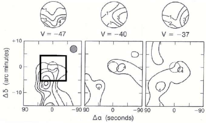
Figure 3: Adapted from Troland et al. 1985 (resolution 2.5’). The three panels show the radial velocities which contribute to the CO emission. In the upper three sketches, the coverage of the CO emission over the face of Cas A is shown. As in Fig 2, most of the CO emission is to the south of the center of Cas A. In each lower panel the thin circle at offset (0,0) marks the edge of the continuum emission from Cas A. The FWHP beam is shown in the upper right of the V=-47 km s^-1 panel. The contour units are peak line intensity in K. The thick square box in this panel shows 1.2 times the boundaries of the 450 $\mu$m sub-mm dust continuum map of Dunne et al. 2003. These data show that the clouds covering the southern part of Cas A are the edges of larger molecular clouds.

2.2 Quantitative Masses and Column Densities

2.2.1 Hi Clouds

There is no ¹³CO  cloud coincident with sub-mm dust clump ‘4’. Clump ‘2’ was included in the ¹³CO  mapping. There is a significant amount of Hi absorption toward most of Cas A. Bieging et al. (1991) have imaged the Hi with an angular resolution of 7^′′. The cloud they have labeled as $A$ (maximum optical depth, $\tau$ of 3 at $v_{LSR}$=-49.7 km s^-1) overlaps with the sub-mm dust peak we labeled as ‘2’. The Hi cloud that Bieging et al. (1991) labeled $D$ ($\tau$=2 and $v_{LSR}$=-43.9  km s^-1) overlaps with the sub-mm dust peak we labeled as ‘1’. In addition, Bieging et al. (1991) find a cloud labeled $B$ that covers the entire continuum source.

From, e.g., Rohlfs & Wilson (2003) the relation between Hi line parameters and Hi  column density, N, is ${\rm N}=1.822\times 10^{18}{\rm T_{s}}\,\int\tau{\rm d}v$. Here $\tau$ is the Hi optical depth, $v$ is the radial velocity in  km s^-1 and T_s is the spin temperature. From the data of Bieging et al. (1991), it is difficult to determine the value of T_s. If the Hi  spin temperatures are $\sim$20 K, and the linewidths are 3.3  km s^-1 (the average $\Delta$V of the ¹³CO ), the column densities of the Hi clouds are $\sim$10²⁰cm^-3. This value is $<$10% of the average column density estimated for the sub-mm dust peaks. Our estimate of the Hi column density is a minimum. It is possible that the values of T_s and $\Delta$V are larger, so that the column density of the Hi would be larger. It is unclear whether the column density of Hi could be as much as a factor of 10 larger. If it were, one could assign all of the sub-mm dust emission to the interstellar medium. For this, one would need a secure determination of the spin temperature of the Hi . Until this is done, one must conclude that while some of the sub-mm dust peaks measured by Dunne et al. (2003) are interstellar, ‘2’ and ‘4’ could be located inside the SNR.

2.2.2 ¹³CO  Clouds

From the ¹³CO  data the beam averaged column densities of these groups of clouds are 6.6 10²¹ cm^-2 (A, B and C), and 2.4 10²¹ cm^-2 (F, G and H). As noted by Wilson et al. (wil (1993)) and Batrla et al. (bat (1984)), the interstellar clouds toward Cas A show indications of clumping on scales down to the respective beam sizes. Thus the beam-chopped measurements of sub-mm dust emission would have recorded these clouds.

In Table 1, we have taken the measured cloud FWHP sizes and average H₂ densities from Wilson et al. (wil (1993)); these are shown in Fig. 1 as shaded circles. Wilson et al. (1993) had used the average H₂ densities (Col. (4) of Table 1), with the FWHP gaussian sizes (Col. (2) of Table 1) to determine masses. Walmsley & Panagia (1978) favor a procedure that uses radii obtained from the assumption of a spherical source shape. In this model, if the beam size is much smaller than the source size, the diameter is 1.47 times the FWHP size (see e.g., the Appendix of Mezger & Henderson (1967)). In addition, we used a factor of 1.36 to account for the mass in helium. The gas masses are given in Col. (5) of Table 1; from a gas-to-dust mass ratio of 100 we obtain dust masses in Col. (6) of Table 1 and Table 2.

2.2.3 Dust Clouds

To determine the dust masses of individual clumps from the integrated sub-mm intensities, we used the 450 $\mu$m contours in Fig. 4 of Dunne et al. (2003). We measured the integrated intensities by digitizing contours, converting to an autocad file to measure the areas enclosed by each of the contours. This does not include contours below 3$\sigma$, since these were not in Fig. 4 of Dunne et al. (2003). Although an underestimate of the actual total integrated flux, this is adequate to obtain the relative flux densities for the clumps. We divided the contours along the depressions to separate clumps (dotted lines in Fig. 1) to obtain the 450 $\mu$m integrated flux densities for the individual clumps. From these we obtained fractional values; when multiplied by the total masses (tabulated in Table 1 of Dunne et al. 2003) we obtained the dust masses for the clumps.

2.2.4 Comparison of ¹³CO  and sub-mm dust masses

We compare the dust masses from the 450 $\mu$m and ¹³CO  data for the overlapping clouds in Table 2. To compare the masses from sub-mm dust emission with ¹³CO  line emission, we must have 450 $\mu$m absorption coefficients for the conversion from thermal dust intensity to mass, that is, values of $\kappa_{450}$. Dunne et al. (2003) argued that they must use a large value, $\kappa_{450}$=1.5 m² kg^-1, which corresponds to an amorphous or clumpy dust structure, to avoid having too much dust produced in Cas A. We used this value to obtain the masses in Col. 3 of Table 2. The value for newly formed dust, in e.g., reflection nebulae or planetary nebulae, 0.88 m² kg^-1, was used to obtain the masses in Col. 4, and the value 0.26 m² kg^-1, for diffuse ISM, was used to obtain the masses in Col. 5. The $\kappa_{450}$ for diffuse ISM, in Col. 5, is the best match to the sub-mm dust mass obtained from ¹³CO  data, in Col. 6.

Table 1: Masses from ¹³CO  Emission

(1)	(2)	(3)	(4)	(5)	(6)
13CO	Radius	Spherical	H2	Gas	Dust
Cloud	(FWHP)	Radius	density	Mass	Mass
Name	(′′)	(pc)	(cm-3)	M⊙	M⊙
A	40	0.43	1000	22	0.2
B	60	0.65	1000	77	0.8
C	20	0.22	400	1	0.01
E	50	0.54	1000	44	0.4
F	65	0.70	1000	100	1.0
G	85	0.89	2000	400	4.0
H	40	0.42	$<$800	$<$17	0.2

Table 2: Dust Masses from both 450 $\mu$m dust and ¹³CO  emission

(1)	(2)	(3)	(4)	(5)	(6)
13CO	Dust	Dust Mass	Dust Mass	Dust Mass	Dust Mass from 13CO
Cloud	Cloud	(amorphous)	(newly formed)	(diffuse ISM)
Name	Name	($\kappa_{450}$=1.5 m2kg-1)	($\kappa_{450}$=0.88 m2kg-1)	($\kappa_{450}$=0.26 m2kg-1)
		M⊙	M⊙	M⊙	M⊙
A, B, C	1	0.2	0.3	1.2	1.0
E	3	0.2	0.3	1.0	0.4
F, G, H	5	0.7	1.2	4.0	5.1

3 Discussion

3.1 Dust toward and in Cas A

We have argued that at least one half of the mass of dust measured toward Cas A is in foreground interstellar clouds. Thus the dust mass quoted by Dunne et al. (2003) should be reduced by at least a factor of 2. Taking the favored value from Dunne et al. (2003), we find that Cas A produced at most 1.5 M_⊙ of dust if we use the sub-mm dust absorption coefficient favored by Dunne et al. (2003). Some additional support for identifying the dust with CO clouds is obtained from a comparison of gas and dust temperatures. As reported by Dunne et al. (2003), most of the mass contained in dust is cold, with a temperature of 18 K. This is consistent with the peak temperatures of the CO measured toward Cas A, $\sim$20 K (Wilson et al. wil (1993)) and the rotational temperature of NH₃, about 18 K (Batrla et al. bat (1984).

The NH₃ molecule is easily dissociated, whereas the CO is much more robust, and so is present throughout molecular clouds. Thus the NH₃ should be present only in cores of clouds; the VLA measurement of NH₃ absorption toward Cas A (Gaume et al. 1994) directly shows this is so. From the equality of the CO and NH₃ temperatures, the clouds are isothermal. In addition, the dust and gas temperatures are very similar. In most cases, this indicates a close coupling of dust and gas, implying densities of order 10⁴ cm^-3, higher than the average for ¹³CO  clouds in Table 1, 400 cm^-3 to 2000 cm^-3. This may indicate denser cores in these clouds. The average minimum dust temperature found for extended cirrus clouds (Lagache et al. 1998) is 17.5 K. If the clouds are very clumpy, the heating may extend to the interior and thus allow us to explain the equality of gas temperatures in spite of the relatively small H₂ densities. If the cores of these clouds are heated by photons, there is an unsolved problem of the dissociation of NH₃. In a comparison of large and small galactic clouds Turner (1995) has found the abundance of NH₃ in clouds similar to those measured toward Cas A is too large compared to his model predictions, so additional production mechanisms for NH₃ are needed.

3.2 General Comments

Morgan & Edmunds (mo2 (2003)) have pointed out that there are a large number of dusty galaxies measured with redshift $z=3$. These authors have produced a model for dust production which shows significant differences when compared to the model of Dwek (dw2 (1998)), showing that predictions are rather parameter dependent. However, since the production of dust in Red Giant stars is slow, this production path would require a very large star formation rate. Thus, supernovae may be the production sites for dust in the early universe. However, a number of questions remain. The first point (raised by Dunne et al. (dun (2003))), is the following. Using a sub-mm dust absorption coefficient which is characteristic of the diffuse ISM gives rise to a very large dust mass. To arrive at their favored dust mass estimate, Dunne et al. (dun (2003)) used an absorption coefficient for amorphous dust or for dust aggregates. Following this approach, but in much more extreme way, Dwek (dw1 (2004)) attributes the sub-mm dust thermal emission from SNe found by Dunne et al. (dun (2003)) and Morgan et al. (mo1 (2003)) in terms of emission by conducting needles. According to Dwek (dw1 (2004)), these are more efficient emitters of sub-mm thermal continuum radiation. If so, the dust mass would be reduced by factors of 10³ or more. Another, less extreme, model of dust emission from the Kepler SNR is that of Contini (cont (2004)). In this model only very large grains survive in the harsh SNR environment. These are more efficient emitters in the mm/sub-mm wavelength range, so the total mass of dust would be a factor of 10 smaller, but this model can fit all of the existing broadband dust measurements. From a comparison of 24 $\mu$m, 70 $\mu$m and sub-mm dust emission images, Hines et al. (2004) note that if the dust emitting at sub-mm wavelengths resides within the SNR, it must have very different properties from the dust emitting in the mid-IR.

If the Dwek supposition is correct, the spectral index of the SNR dust must be different from that of typical interstellar dust. Then, with $\sim$15^′′ resolution far-IR images, for example with the PACS imaging photometer instrument on Herschel or the HAWC far IR bolometer camera on SOFIA, one should be able to map the spectral indices of thermal dust emission across Cas A and and toward the nearby clouds. If one could distinguish between interstellar dust and dust inside the SNR, this would be evidence for different properties. Such a finding would have very far-reaching consequences for the mass of dust produced by SNRs. Another future line of investigation involves a study of the properties of the interstellar clouds near the edges of the Cas A SNR. The presence of line wings in CO or a change of excitation in ¹³CO  might indicate an interaction of the clouds and the SNR. Although not directly related to Cas A, an image of a larger region near the SNR in both ¹³CO  lines and sub-mm dust emission would allow a more complete determination of cloud properties.

4 Conclusions

From a comparison of the distribution of the image of integrated J=1–0 ¹³CO  line emission (Wilson et al. wil (1993)) with the image of 450 $\mu$m dust emission (Dunne et al. dun (2003)), we find positional agreement for 3 of 6 maxima. One sub-mm dust peak, ‘2’ was not mapped in ¹³CO , while another, ‘6’ lies outside the forward shock of the SNR. The third prominent dust emission peak, ‘4’ does not show ¹³CO  emission. There is Hi absorption at this position, but the column density of Hi may not be sufficient to account for the dust emission, so this may be inside the SNR. Both the ¹³CO  and sub-mm dust images show that the emission is concentrated south of the center of Cas A, while the synchrotron emission is a rather symmetric ring-shaped structure. There is good agreement between the masses of the sub-mm dust maxima coincident with the ¹³CO  peaks and also good agreement between the dust temperature and the peak molecular line temperatures from CO and NH₃. We conclude that at least one-half of the dust emission measured toward Cas A arises from molecular clouds toward, but not inside the SNR. From the conversion favored by Dunne et al. (dun (2003)) and our corrections for dust in line-of-sight molecular interstellar clouds, we find that the mass of dust inside the SNR is at most 1.5 M_⊙.

acknowledgement We thank C. M. Walmsley and a referee for valuable comments.

References

- (1) Batrla, W., Walmsley, C.M., Wilson, T.L. 1984 A & A 136, 127
- (2) Bieging, J.H., Goss, W.M., Wilcots, E.M. 1991 ApJS 75, 999
- (3) Contini, M. 2004 A & A submitted (astro-ph/0404262 v1)
- (4) Dunne, L., Eales, S., Ivison, R., Morgan, H., Edmunds, M. 2003 Nature 424, 285
- (5) Dwek, E. 2004 accepted by ApJ (astro-ph/0401074 v2)
- (6) Dwek, E. 1998 ApJ 501, 643
- (7) Eales, S, Bertoldi, F., Ivison, R., Carilli, C.L., Dunne, L.,Owen, F. 2003 MNRAS 344, 169
- (8) Emerson, D.T., Klein, U., Haslam, C.G.T. 1979 A & A 76, 92 (EKH)
- (9) Gaume, R.A., Wilson, T.L., Johnston, K.J. 1994 ApJ 425, 127
- (10) Hines, D. C., et al. 2004 ApJS 154, 290
- (11) Johnstone, D., Wilson, C.D., Moriarty-Schieven, G., Giannakopoulou-Creighton, J., Gregersen, E. 2000 ApJ Suppl 131, 505
- (12) Lagache, G., Abergel, A., Boulanger, F., Puget, J.-L. 1998 A & A 333, 709
- (13) Liszt, H., Lucas, R. 1999 A & A 347, 258
- (14) Loinard, L., Lequeux, J., Tilanus, R.P.T. Lagage, P.O., 2003 Rev. Mex. A & A 15, 267
- (15) Mezger, P. G. & Henderson, A. P. 1967 ApJ 147, 471
- (16) Morgan, H.L., Dunne, L., Eales, S.A., Ivison, R.J., Edmunds, M.G. 2003 ApJ 597, L33
- (17) Morgan, H.L., Edmunds, M.G. 2003 MNRAS 343, 427
- (18) Panagia, N., Walmsley, C. M. 1978 A & A 70, 411
- (19) Rohlfs, K., Wilson T. L. 2003 Tools of Radio Astronomy, 4th edition, Springer-Verlag, Heidelberg
- (20) Smail, I., Ivison, R.J., Blain, A.W. 1997 ApJ 490, L5 bibitem[1985]tro Troland, T., Crutcher, R.M., Heiles, C., 1985 ApJ 298, 808
- (21) Turner, B.E. 1995 ApJ 444, 708
- (22) Wilson, T.L., Mauersberger, R., Muders, D., Przewodnik, A., Olano, C. 1993 A & A 280, 221
- (23) Wilson, T.L., Rood, R. T. 1994 Ann Rev A & A 34, 191
- (24) Wright, M., Dickel, J., Koralesky, B., Runnick, L. 1999 ApJ 518, 284