Ultrahigh Energy Nuclei Propagation in a Structured, Magnetized Universe

Abstract

We compare the propagation of iron and proton nuclei above $10^{19}\,$eV in a structured Universe with source and magnetic field distributions obtained from a large scale structure simulation and source densities $\sim 10^{-5}\mbox{Mpc}^{-3}$. All relevant cosmic ray interactions are taken into account, including photo-disintegration and propagation of secondary products. Iron injection predicts spectral shapes different from proton injection which disagree with existing data below $\simeq 30\,$EeV. Injection of light nuclei or protons must therefore contribute at these energies. However, at higher energies, existing data are consistent with injection of pure iron with spectral indices between $\sim 2$ and $\sim 2.4$. This allows a significant recovery of the spectrum above $\simeq 100\,$EeV, especially in the case of large deflections. Significant auto-correlation and anisotropy, and considerable cosmic variance are also predicted in this energy range. The mean atomic mass $A$ fluctuates considerably between different scenarios. At energies below 60 EeV, if the observed $A\gtrsim 35$, magnetic fields must have a negligible effect on propagation. At the highest energies the observed flux will be dominated by only a few sources whose location may be determined by next generation experiments to within $10-20^{\circ}$ even if extra-galactic magnetic fields are important.

I Introduction

Ultra-high energy cosmic rays (UHECRs) are particles of energy $\geq~{}10^{19}$ eV, which give rise to spectacular air showers spreading over square miles when reaching the Earth’s lower atmosphere, but whose properties are at the moment poorly known because of low fluxes scaling roughly as $E^{-3}$. A recent review on the experimental and theoretical aspects of this topic can be found, for example, in Ref. review .

As the Auger Observatory auger-design-report is still in a phase of deployment and early analysis, most of the current data come from two experiments relying on different techniques, the High Resolution (HiRes) “Fly’s Eye” fluorescence telescopes and the AGASA ground array. The first technique consists in observing the development of the longitudinal extent of the air shower through the atmospheric fluorescence yield, whereas arrays reconstruct the lateral development of the shower, by detecting secondary products reaching the ground level.

Because of large experimental systematics in energy determination for both methods, and because of low statistics at the highest energies, the flux of UHECRs is still poorly known. Whereas AGASA does not see any cut-off in the energy spectrum even at $10^{20}$ eV agasa-spectrum , recent results of HiRes indicate a cut-off above around $10^{19.8}\,$eV hires-spectrum .

The nature of the primary particles is even less clear. AGASA sets an upper limit on the photon fraction of $\leq 28\%$ at $10^{19}$ eV agasa-photons , but it is experimentally difficult to discriminate between light and heavy nuclei: various methods give results which are largely dependent on hadronic models and on experimental uncertainties, leading to discrepancies in the results watson-compo .

Concerning the arrival directions, all the data accumulated until now are roughly consistent with isotropy, at least on large angular scales. However, particularly at the highest energies, the lack of statistics still allows a substantial large-scale anisotropy of the UHECR sky. On small scales (a few degrees), AGASA has detected a clustering of events agasa-clusters but its statistical significance remains questionable finley . Furthermore, the HiRes experiment didn’t confirm this feature hires-clusters , but the integrated aperture of HiRes stereo data is still lower than that of AGASA.

The Pierre Auger Observatory which is currently under construction will within a few years accumulate a statistics on UHECRs at energies above $10^{19}$ eV which will be orders of magnitude above previous experiments. The resulting spectrum, arrival direction map and perhaps composition should therefore put serious constraints on UHECR origin and propagation models. This provides a motivation for investigating a wide variety of UHECR scenarios consistent with current data.

Various exotic models for the UHECR origin have been proposed bs , particularly in light of the possible absence of the Greisen-Zatsepin-Kuzmin (GZK) “cut-off” gzk as claimed by AGASA. However, the experimental situation about the spectrum remains unsettled and classical “astrophysical” scenarios remain completely plausible. These models are based on particle acceleration at shocks in powerful extragalactic astrophysical objects, ranging from compact objects such as $\gamma-$ray bursts (GRBs) to large-scale radio lobes of active galactic nuclei (AGNs), see for example Ref. torres-review . They have the obvious advantage to be exclusively based on known physics and astrophysical objects. They should therefore be tested extensively before a possible rejection in light of more speculative scenarios.

Much work has already been carried out in the framework of astrophysical scenarios. Various models for sources and particle propagation predict different observables such as the spectrum or anisotropies of UHECRs observed on Earth. A major feature of UHECR propagation models is the strength and extension of extragalactic magnetic fields (EGMF) which can give rise to important deflections depending on particle charge and energy. The EGMF are mostly unknown at present vallee and different models for these fields can lead to different predictions, as the comparison between Refs. lss-protons ; sme-proc and Ref. dolag shows. In Ref. lss-protons , the authors use magnetic fields derived from a cosmological large scale structure (LSS) simulation with magnetic fields generated at the shocks that form during LSS formation, whereas in Ref. sme-proc and Ref. dolag fields of “primordial” origin have been considered. While the different models for initial magnetic seed fields produce different large scale magnetic field distributions and, therefore, lead to different predictions for UHECR deflection, there is still a significant discrepancy between Ref. lss-protons ; sme-proc and Ref. dolag , hinting that other technical reasons may play a role here.

The goal of this article is to extend previous work on proton propagation in Ref. lss-protons to the case of iron sources. This allows to fill a gap in the range of plausible models before Auger data will discriminate between various possibilities. The Hillas criterion hillas shows qualitatively that heavy nuclei can be accelerated to higher energies than protons because their gyroradii in the magnetized accelerator are smaller. Injection of heavy nuclei can therefore plausibly contribute to the observed UHECR flux at the highest energies.

Heavy nuclei propagation has already been considered previously heavy : Discrete sources at given distances were studied with and without unstructured magnetic fields bertone . A model with discrete and continuous source distributions and magnetic fields with a uniform Kolmogorov distribution was developed in Ref. yamamoto . In Ref. sigl-iron , heavy nuclei propagation was studied for magnetized individual sources.

In the present paper, we consider the following scenario, largely inspired by the “best-fit model” which was presented in Ref. lss-protons : The sources are distributed according to the baryon density obtained from a LSS simulation of a typical local universe miniati . Their density, $n_{s}\simeq 2.4\times 10^{-5}\mbox{Mpc}^{-3}$, corresponds to average distances between sources of $\simeq 40\,$Mpc, comparable to typical UHECR interaction lengths at GZK energies. Therefore, neither the continuous source approximation nor the “universal spectrum” discussed in Ref. aloisio is applicable to this case. Source densities of this order of magnitude are motivated by $i$) comparable densities of candidates for powerful accelerators such as AGNs and $ii$) the fact that they appear necessary to explain the small-scale clustering observed by AGASA kachelriess ; lss-protons ; blasi . The observer is located in a void next to a supercluster of matter, to mimic our local extragalactic environment. The magnetic fields there are weak, although an experimental estimate of such a quantity in our immediate surroundings (i.e. within a few Mpc) is lacking. However, magnetic fields of the order of a $\mu$G in galaxy clusters are present and sufficient to significantly deflect high energy charged particles.

We do not take into account galactic magnetic fields in the work presented here, although they might play a significant role in the degradation of anisotropy signals for iron even at super-GZK energies. Previous studies, e.g. Ref. yoshi-galdeflec , show that galactic and halo fields spread arrival directions by an angle depending on energy, composition and arrival direction relative to the galactic center.

The configuration studied, namely rare sources, structured magnetic fields, and the presence of nuclei at injection, complicates the simulations. The numerical techniques and difficulties are presented in Sect. II. In Sect. III we turn to the results obtained with proton injection, and in Sect. IV we study iron injection in the case of negligible deflection. Both Sects. III and IV describe useful reference cases. The scenario with iron injection including the EGMF obtained from the LSS simulation of Ref. miniati is developed and interpreted in Sect. V. Finally, we conclude in Sect. VI.

II Simulations and Methods

The numerical framework for our simulations is similar to the one described in some details in Ref. lss-protons . Therefore we will here only remind the reader of the major features of the technique, and present some specific remarks concerning problems raised by the study of heavy nuclei propagation.

II.1 Magnetic fields and propagation

The cosmic environment, i.e. the magnetic field as well as the baryonic density which defines the source distribution are the same as described in Ref. lss-protons . They have been computed according to a simulation of large scale structure formation. An extensive discussion of the numerical modeling of the magnetic field was presented already in Ref. lss-protons ; sme-proc . Here it suffices to say that the magnetic fields are generated at cosmic shocks according to the Biermann battery mechanism and are then renormalized at the end of the simulation so that for a Coma-like cluster the average magnetic field in the core would be of order of a $\mu$G. An alternative mechanism to generate magnetic fields at shocks is provided by the Weibel instability weibel59 . According to recent investigations of this process silva03 ; schlick03 , magnetic fields with strength amounting to a sizable fraction of the thermal energy can be produced at cosmic shocks on very short time scales (of order of the inverse of the electron plasma frequency). In any case, an important feature of our LSS simulation is the existence of $\sim 0.01-1\mu$G scale EGMF extending over scales of several Mpc in and around galaxy clusters. In contrast, EGMF in the voids are $\lesssim 10^{-5}\,\mu$G, negligible for UHECR deflection. Importantly, the resulting EGMF is consistent with statistics of existing Faraday Rotation Measures with lines of sight through filaments, despite the fact that the magnetic field strength can be close to equipartition value with the total energy of the gas ryu . We therefore have a strongly structured EGMF, different from the idealized case of a field with a Kolmogorov spectrum with spatially constant parameters used in Ref. bertone .

Our EGMF also differ from those resulting from uniform initial seeds, in that the latter appear to be more concentrated in the core of collapsed structures sme-proc ; dolag . However, while a more concentrated field produces less deflection of UHECRs, at least the results from the model in Ref. sme-proc indicate that such as difference is not dramatic. Different numerical models predict different results though. Unfortunately, the behavior of the magnetic field with distance from the cluster center is not known. The current data indicate that $\mu$G strong magnetic fields extend out to at least $\sim 1$ Mpc clarke and possibly to larger distances johnston . At distances above $1\,$Mpc from a cluster core, however, probing the magnetic fields becomes extremely difficult because the Faraday Rotation Measure loses sensitivity in low density regions. Furthermore, the intracluster magnetic field topology is also poorly known, although the situation will likely improve in the future.

The size of the LSS box used in our simulations is $\sim 75\,$Mpc, with a grid of $5123$ comoving cells. The observer, modeled as a sphere of 1.5 Mpc radius, is placed at the border of a void, not far from a massive and magnetized structure which mimics the Virgo cluster. To enhance CPU efficiency and allow at the same time to have particles reaching the observer from regions further than 75 Mpc, we use periodic boundary conditions in the simulation to duplicate the allowed propagation region of UHECRs.

To take into account the “cosmic variance” which arises because of various possible source locations relative to the observer, we simulate different realizations, for which the position of 10 sources are chosen at random within the box, with probability proportional to the baryon density. Iron nuclei or protons are injected isotropically from each of these random sources in the simulation.

Nuclei interactions are treated as described in Ref. bertone : We take into account photo-disintegration, pion production and pair production on the low energy photon backgrounds. Deflection is computed by solving the Lorentz equation of motion: For this purpose we use a Bulirsch-Stoer integrator with adaptive stepsize.

In order to measure properly the all-particle spectrum at the observer position, we need to keep track of every secondary particle during the propagation. One nucleus emitted by a source can therefore generate up to 56 nucleons after a propagation time depending mostly on primary energy. When recording an “event”, no distinction is made between primary and secondary particles, but the properties of the particle, namely its charge and mass, are recorded.

After propagation, the analysis of simulated events is performed for each simulated data set, roughly in the same way as in Ref. lss-protons : Taking into account fluctuations in the spectra and intensities of the sources, we build observed energy spectra, average composition plots, deflection histograms, typical sky maps, auto-correlation functions and full-sky angular power spectra (partial sky coverage being in theory invertible as shown in Ref. deligny ). In the present study we neglect any finite experimental resolution in energy and arrival directions. The “cosmic variance” associated to fluctuations in source positions and properties within the scenario is also computed for these observables. It is in general defined as the one-sided median deviation from the average of the considered quantity. The fluctuations of the source properties are chosen as in Ref. lss-protons : Each source is characterized by a spectral index $\alpha_{i}$ and a luminosity $Q_{i}$ with

$$\frac{dn_{s}}{dQ_{i}} \propto Q_{i}^{-2.2}\;\;\mbox{for}\;\;1\leq Q_{i}\leq 100\,,$$ (1)

$$\frac{dn_{s}}{d\alpha_{i}} = \mbox{const.}\;\;\mbox{for}\;\;\langle\alpha\rangle-0.1\leq\alpha_{i}\leq\langle\alpha\rangle+0.1\,.$$

Here, $\langle\alpha\rangle$ will be chosen to best fit the observed spectrum. Finally, we assume that all sources accelerate to a common maximal energy $E_{\rm max}$ for which we will choose different values.

II.2 Numerical Difficulties

Our simulations allow detailed simultaneous predictions of various observables in specific scenarios. The drawback is of course a large CPU time consumption: The ratio of simulated trajectories over recorded events is large, of order 1000 or more depending on the considered scenario. In the case of nuclei propagation, and for the EGMF we use, the recorded event yield is particularly low because of large deflections and the necessity to follow secondary nuclei.

Unfortunately, backtracing the particles from the observer does not allow to predict observables for the model, since we do not know in advance the spectrum, composition, and effective source distribution of observed events, not to mention the stochastic nature of cosmic ray interactions.

The consequence of CPU limitations is the limited statistics of simulated events. As we want to simulate many source realizations for different scenarios (typically around 100 source location realizations for each scenario), we restricted ourselves to $10^{4}$ events per realization, above either 10 EeV or 40 EeV. This is sufficient as a first step, since our goal is to explore the widest range of possible scenarios rather than to focus on one specific model, which we might choose later in the light of Auger results. In the future, we plan to carry out more detailed simulations using a parallel version of the cosmic ray propagation code currently under development.

II.2.1 Event Reweighting

For CPU efficiency, we inject particles at the sources with a uniform distribution in the logarithm of energy. To predict observables with fluctuating source luminosities $Q_{i}$ and spectral indexes $\alpha_{i}$, we reweight each simulated trajectory with a factor that depends on the source power and the injection spectrum. This reduces the effective number of events for statistical quantities such as histograms and the anisotropy observables. Reweighting can also bias the event maps by causing spots to appear on the maps.

We show here as an example how applying weights to simulated trajectories reduces the sensitivity of the angular power spectrum to large-scale anisotropies.

• Absence of weights. Given $N$ arrival directions $\vec{n}_{i}$ distributed on the sphere, we define our estimator of the $C_{\ell}$ by $a_{\ell m}~{}=~{}N^{-1}\sum_{i=1}^{N}Y_{\ell m}(\vec{n}_{i})$ and $C_{\ell}~{}=~{}(2\ell+1)^{-1}\sum_{m=-\ell}^{\ell}|a_{\ell m}|^{2}$, where $Y_{\ell m}(\vec{n}_{i})$ are the usual spherical harmonics. For the null hypothesis of full isotropy, the mean value for this estimator becomes

  $$\left<C_{\ell}\right>=\frac{1}{(2\ell+1)\,N^{2}}\sum_{m}\sum_{i,j}\left<Y_{\ell m}(\vec{n}_{i})Y_{\ell m}^{*}(\vec{n}_{j})\right>\,.$$

  As the arrival directions are independent, only the terms $i=j$ contribute, for which $\left<|Y_{\ell m}(\vec{n}_{i})|^{2}\right>=(4\pi)^{-1}\int d\Omega|Y_{\ell m}(\vec{n})|^{2}=(4\pi)^{-1}$, and therefore, one finds the well-known result

  $$\left<C_{\ell}\right>=\frac{1}{4\pi N}\,.$$ (2)

• Effect of weights: Let us now assign weights $\omega_{i}$ to the events, with a distribution $p(\omega)$ with mean $\mu$ and standard deviation $\sigma$. The first average to consider is over arrival directions. The computation is the same as before, but since the definition of the estimator is now $a_{\ell m}~{}=~{}\left(\sum_{j}\omega_{j}\right)^{-1}\sum_{i}\omega_{i}Y_{\ell m}(\vec{n}_{i})$, it follows that $\left<C_{\ell}\right>~{}=~{}(4\pi)^{-1}\left(\sum\omega_{i}^{2}\right)\left(\sum\omega_{i}\right)^{-2}$. The next step is to average over the weight distribution, which is independent of arrival direction distribution. We place ourselves in the limit of large $N$, therefore replacing the sums over $\omega_{i}$ by integrals. This leads immediately to

  $$\left<C_{\ell}\right>=\frac{1}{4\pi N_{\mbox{\tiny{eff}}}}\,,\;\;\;\;\mbox{where}\;\;\;\;N_{\mbox{\tiny{eff}}}=\frac{N}{1+\left(\frac{\sigma}{\mu}\right)^{2}}\,.$$ (3)

This last formula shows that if the weight distribution is broad, i.e. $\sigma/\mu\gtrsim 1$, the effective number of arrival directions becomes small as the only events which will be “counted” are the ones with the largest weights. This results in an increase of the bias in the power spectrum estimate in the isotropic case, and the sensitivity to possible small anisotropies in the model is reduced.

II.2.2 Effect of Finite-Sized Observer and Simulation Box

The ideal observer in the method developed here should be point-like, but, once again for CPU reasons, we modeled the observer as a sphere of radius $1.5$ Mpc. There is in general no problem with this procedure, as we expect the UHECR properties such as density, spectrum, composition, and anisotropies to be roughly the same within this volume. This is because the sources are extragalactic and typically located at distances of tens to hundreds of Mpc, and the magnetic field around the observer is very weak, $\sim$10 pG. However, in some realizations for the source locations, one or a few sources can be located within a few Mpc from the observer, and the finite size of the observer “spreads” the image of such sources over a few degrees. This smoothes out the auto-correlation function in the first few bins of small angular off-set. For the case of propagation in a regime with considerable deflection, this effect is, however, of little importance.

The finite size of the simulation box can also lead to spurious effects observable on simulated sky maps. For events at the lowest energies, $E\sim 10\,$EeV, when particles travel over large distances and in the absence of deflections by magnetic fields, an excess of events is observed in the direction of the simulation box corners because of the rectangular geometry of the box, and the periodic repetition of sources can be observed in the sky maps of arrival directions within a given source realization. However, for the cases of interest in our simulations, energies $E\gtrsim 40\,$EeV and/or non-negligible magnetic fields, these effects disappear completely.

II.2.3 Specificities of Heavy Nuclei Propagation

There are a number of difficulties which arise when studying heavy nuclei and their secondaries in the framework of our method, in particular concerning the analysis of angular distributions for simulated events.

Figure 1: Histogram of injection energies of events detected by the observer in a scenario with iron injection. The injection spectrum is flat in the logarithm from 10 EeV to 10 ZeV, but evidently this is not the case for the detected events. This effect is explained in the text below.

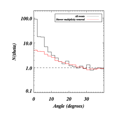
Figure 2: Auto-correlation of events with energies above 80 EeV for a realization of iron injection with magnetic fields, without (black) and with (red) correction for nuclear showers arising from the disintegration of a single iron near the observer. ${\cal N}(\theta)=1$ (dashed line) corresponds to an isotropic distribution.

• Propagation of nuclei takes more CPU time than protons because the deflections are larger, which leads the Bulirsch-Stoer integrator to choose smaller stepsizes for integrating the trajectories.

• For heavy nuclei injection, a consequence of photo-disintegration processes is that particles with a given observed energy have an extremely large range of injection energies. Fig. 1 shows the distribution of injection energies for recorded events. Two populations appear clearly: 1) At low injection energies, the flat distribution of iron originating from nearby sources which is the same as in the case of proton injection; 2) Nuclei emitted at the highest energies which are detected as light nuclei after having undergone photo-disintegration. Due to the approximate conservation of the Lorentz factor in interactions, this population appears at injection energies $E\geq A\times E_{min}$, which corresponds to $\log(E/EeV)\geq 2.75$, as seen in Fig. 1. Note that the dip between these two regions is an artifact due to the fact that iron at those energies undergo frequent photo-disintegrations but their secondary protons have energies below $E_{\rm min}$ and, therefore, are not detected. This affects the reconstruction of the injection spectrum in that region.

  As events are reweighted according to their injection energies, the situation depicted above leads to a broad weight distribution. Therefore, the problems raised previously are particularly acute for iron injection.

• Although they are necessary to evaluate the spectrum and composition, “showers” of nuclei which are generated from a single iron near the observer create fake signals in the auto-correlation. A crude but efficient approach to this problem is to use only the first particle of each shower (composed of 56 particles at most) in the anisotropy analysis, or equivalently to assign to each particle a weight inversely proportional to the size of the shower it belongs to. An example is shown in Fig. 2, where the auto-correlation is computed with and without reweighting of showers, using the estimator lss-protons

  $${\cal N}(\theta)=\frac{C}{S(\theta)}\sum_{j\neq i}\left\{\begin{array}[]{ll}\omega_{i}\omega_{j}&\mbox{if $\theta_{ij}$ in the bin of $\theta$}\\ 0&\mbox{otherwise}\end{array}\right\}\,.$$ (4)

  Here, $S(\theta)$ is the solid angle size of the corresponding bin, and $\omega_{i}$ are weights as before. The normalization factor $C=\Omega_{e}/\sum_{j\neq i}\omega_{i}\omega_{j}$, with $\Omega_{e}$ denoting the solid angle of the sky region where the experiment has non-vanishing exposure, is chosen such that an isotropic distribution corresponds to $N(\theta)=1$.

We point out that in terms of CPU time consumption, the scenarios explored in this paper are perhaps the most challenging for obtaining sufficient statistics. This is the result of combining heavy nuclei propagation with considerable magnetic fields and a discrete distribution of rare sources. Indeed, these kinds of scenarios have not been studied yet in great detail because they are computationally time-consuming. However, it is important to perform simulations and to predict observables for those scenarios as they allow to scan a large range of UHECR models.

Injected Number of particles $E_{\rm min}$ $E_{\rm max}$ EGMF realizations Proton 10 EeV 1 ZeV No 39 Proton 40 EeV 1 ZeV No 40 Proton 10 EeV 1 ZeV Yes 19 Proton 40 EeV 1 ZeV Yes 26 Iron 10 EeV 4 ZeV No 100 Iron 10 EeV 4 ZeV Yes 56 Iron 10 EeV 10 ZeV No 200 Iron 40 EeV 10 ZeV No 171 Iron 10 EeV 10 ZeV Yes 78 Iron 40 EeV 10 ZeV Yes 97

Table 1: List of simulations carried out. Each simulation corresponds to $10^{4}$ recorded “events”. To increase the statistics at high energies, some scenarios were simulated twice: once with $E_{\rm min}=10$ EeV, and once with $E_{\rm min}=40$ EeV.

III Warming up: Proton Injection

To have a reference and compare with iron simulations, we extensively simulated proton emission and propagation with parameters similar to the “most-favored” scenario number 6 of Ref. lss-protons . In the framework of this scenario, for a source density of $2.4\times 10^{-5}\mbox{Mpc}^{-3}$, we chose a distribution of sources following the baryon density, with and without EGMF. The maximum injection energy was set to 1 ZeV$=10^{21}\,$eV, and all events above $E_{\rm min}=10\,$EeV are taken into account. The injection spectrum in this energy range was chosen $\propto E^{-\alpha}$, where the average value of $\alpha$ is fitted to the data and typically varies between $\simeq 2$ and $\simeq 2.4$.

The main conclusions from these simulations are:

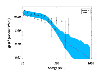
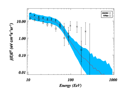
Figure 3: Energy spectra predicted in the case of proton injection at the sources, without (top panel) and with (bottom panel) EGMF. The average (solid line) and cosmic variance (shaded band) result from various realizations of the source properties and locations. The source positions are assumed to have a statistical distribution proportional to the baryon density. For each source location, 50 realizations for source intensity and spectral index are drawn according to the distributions of Eq. (1). The mean source spectral index is $\langle\alpha\rangle=2.4$. To guide the eye we also show the spectra measured by AGASA agasa-spectrum and HiRes hires-spectrum . The normalization of our curves is obtained by adjusting the average spectrum to low energy data.

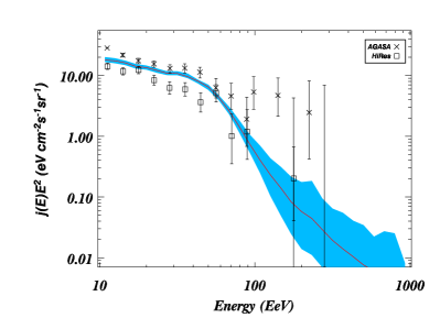
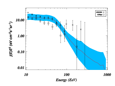
Figure 4: Same as Fig. 3, for proton injection with EGMF fields: In the top panel all sources have the same intensity $Q=1$ and spectral index $\alpha=2.4$, i.e. cosmic variance is only due to fluctuations in the source locations. The bottom panel includes source property fluctuations as in Fig. 3, but with a mean injection spectral index $\langle\alpha\rangle=2.0$ instead of 2.4.

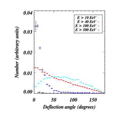
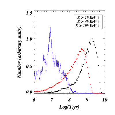
Figure 5: Distributions of deflection angles (top panel) and time delays versus straight-line propagation time (bottom panel) of simulated trajectories for proton injection with spectral index $\alpha=2.4$. The distributions are cumulated over all source location realizations and the error bars are drawn from Poissonian statistics and reflect the finite number of simulated trajectories.

• The predicted energy spectra are shown in Figs. 3 and 4. As expected, in this astrophysical scenario the GZK feature appears at energies above $\sim 4\times 10^{19}\,$eV. Since the sources are distributed at various distances from the observer, the feature does not appear as a sharp cut-off, but rather as a steepening of the spectral index. Let us remark that we are not able to study the ankle within these simulations which are limited so far to energies above 10 EeV. A proton average injection spectral index $\langle\alpha\rangle=2.4$ fits better than $\langle\alpha\rangle=2.0$ to current AGASA/HiRes data at $10<E<40\,$EeV, see Fig. 4.

  A major aspect of the obtained spectra is the presence of a large cosmic variance, which has different origins below and above the GZK feature: Below the GZK feature, this variance is mostly due to source luminosity fluctuations, since it almost disappears if sources have identical properties, see Fig. 4. Above the GZK feature, fluctuations of the source locations also significantly contribute to cosmic variance: The spectrum at post-GZK energies depends substantially on the presence of a few powerful sources close to the observer. This is because our source density is low: No continuous approximation for the source distribution could reproduce such results.

  Finally, the comparison of the upper and lower panels in Fig. 3 demonstrates the effect of EGMF on the spectrum: The attenuation of spectra at high energies is slightly more pronounced in the case of EGMF, the mean spectral slope in the energy range between $\simeq 50\,$EeV and $\simeq 200\,$EeV being $\sim 6.4$ instead of $\sim 5.3$. This is due to the increase of the average traveled distance in the presence of EGMF.

• Deflections and time delays are defined here as the deflection and delay accumulated by UHECRs compared to photons. In general they are very difficult to observe, but $i$) moderate deflections from an unambiguously identified source could be measured, and $ii$) time delays could be measured in case a GRB or a SN explosion can be identified as source. Predicted deflection angle and time delay histograms are shown in Fig. 5. It can be seen that above 10 EeV the deflection distribution obtained is not trivial, i.e. it is not the one we would obtain if particles were in the fully diffusive regime. One can also remark that even at 100 EeV, typical deflections are still of the order of 10-40 degrees. This is due to the fact that EGMF are substantial, and sources are generally located in magnetized areas: particles are mostly deflected in the local environment around their sources. The time delay histogram shows that typical time delays are large, around 1 Gy at 10 EeV, due to the EGMF. Thus in this scenario, even at the highest energies time delays will be too large to be directly measurable.

• Auto-correlation of events. Even for substantial EGMF, the fact that at high energies all events come from a few sources leads to strong auto-correlation signals. A major feature is, however, the high cosmic variance of this auto-correlation, which depends strongly on the positions and luminosities of the sources closest to the observer. This can be seen in Fig. 6 which shows two different source realizations: The first one presents a smooth auto-correlation extending to 30 degrees, whereas in the second realization, with a nearby source, the auto-correlation is highly peaked, with a gaussian-like shape of width $\sigma\sim 5$ degrees.

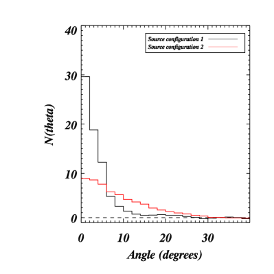
Figure 6: Examples of auto-correlation for $E>100$ EeV for proton injection with spectral index $\alpha=2.4$ and EGMF, for two different source configurations. Within the same model, fluctuations of the distances to the nearest sources from the observer generate extremely different auto-correlation (and therefore clustering) shapes. $N(\theta)=1$ (dashed line) corresponds to an isotropic distribution.

IV Iron Injection Without Magnetic Deflection

This section illustrates general features of heavy nuclei propagation. We do not take into account particle deflections, and, therefore, these results can be compared to the case of small deflections obtained in the EGMF scenarios of Refs. dolag ; yamamoto . Note, however, that deflection can still be of the order of $\sim 20^{\circ}$ in the EGMF scenario of Ref. dolag when their results are extrapolated to nuclei.

IV.1 Spectrum

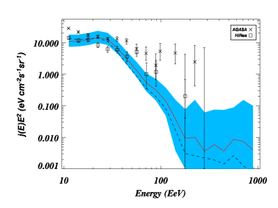
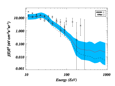
Figure 7: Energy spectra predicted for iron injection without deflection. The average (solid line) and cosmic variance (shaded band) are obtained as in Fig. 3. The average source spectral index is $\langle\alpha\rangle=2.0$, whereas the dashed lines show the average spectrum for $\langle\alpha\rangle=2.4$. The maximum injection energy is set to 4 ZeV (top panel) and 10 ZeV (bottom panel).

In Fig. 7 we represent the spectra obtained with an average iron injection spectral index $\langle\alpha\rangle=2$, and two different maximum injection energies. The injection spectra which allow to fit the observed spectra tend to be somewhat harder than in the case of protons. Clearly, however, the spectral shape predicted at energies $E\lesssim 30\,$EeV is not compatible with observations. At those energies, a lighter component, e.g. from proton injection, is necessary. Around 20-30 EeV a small “bump” is predicted for pure iron injection which is mostly due to secondary sub-GZK protons.

At energies $E\gtrsim 30\,$EeV we observe a flux suppression due to nuclear photo-disintegration. The shape of the cut-off is not the same as in Fig. 3 for proton injection: in particular it starts at lower energies and it is flatter. Furthermore, there is a significant steepening around 100 EeV, with a flattening between $10^{20}$ and $10^{21}$ eV. The location of this flattening or “spectrum recovery” strongly depends on the source configuration, as can be seen from the large cosmic variances in Fig. 7, and also on the maximal injection energy: Fig. 7 shows that the recovery flux is statistically higher when increasing $E_{\rm max}$.

IV.2 Composition

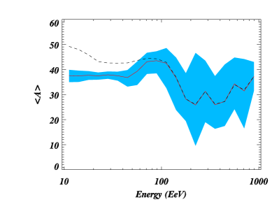
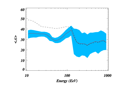
Figure 8: Predicted average atomic mass $\langle A\rangle$ as a function of observed particle energy corresponding to the spectra shown in Fig. 7 for iron injection without deflection. Mean and cosmic variance are computed as in Fig. 7 with $\langle\alpha\rangle=2.0$ and maximum injection energy of 4 ZeV (top panel) and 10 ZeV (bottom panel). The dashed lines show the average composition for $\langle\alpha\rangle=2.4$.

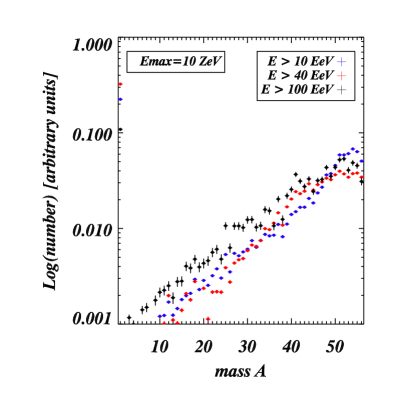
Figure 9: Distributions of masses in the case of iron injection with spectral index $\alpha=2$, $E_{\rm max}=10$ ZeV and no EGMF. The distributions are cumulated over various source position realizations and the error bars are drawn from Poissonian statistics reflecting the finite number of simulated trajectories.

The mean composition as a function of energy is shown in Fig. 8, where the cosmic variance is due to the fluctuations in source locations and properties. At energies $E\lesssim 30\,$EeV, the mean mass $\langle A\rangle$ is typically higher than 35, reflecting in fact a bimodal distribution: At these energies we have on the one hand protons originating from high-energy heavy nuclei photo-disintegration, and on the other hand heavy particles injected and surviving propagation at low energies. If we model the composition as a simple (H,Fe) mixture, which is done in most experimental studies at these energies, the observed $\langle A\rangle\sim 35$ in Fig. 8 corresponds to $\simeq 40$% H and $\simeq 60$% Fe even for pure iron injection. The dashed lines in Fig. 8 represent $\langle A\rangle$ in the case of a different injection spectral index, $\langle\alpha\rangle=2.4$ instead of 2: It is evident that the steeper the injection spectrum, the heavier the composition. Indeed, decreasing $\alpha$ enhances the number of high energy injected iron and, therefore, of low-energy proton secondaries which implies a lighter composition at energies below $\simeq 100\,$EeV.

Between $\simeq 40\,$EeV and $\simeq 200\,$EeV, the situation is less clear as there is a competition between two phenomena: On the one hand, at energies above $\sim 100\,$EeV iron is efficiently photo-disintegrated, whereas below $E_{\rm max}/56$ secondary protons from dissociated iron nuclei appear. Both effects suppress the average atomic mass $\langle A\rangle$. This can lead to a bump around $\simeq 100\,$ EeV provided that the two effects operate in different energy ranges, that is if $E_{\rm max}/56$ is well below $\sim 100\,$EeV, as in the top panel of Fig. 8. In general, these effects are reduced for steeper injection spectral index $\alpha$, as can be seen in Fig. 8, because there are fewer secondary products to affect a larger population of particles in the lower energy part of the spectrum. Therefore, at these transition energies, the mean composition appears to be subject to large fluctuations depending on various parameters.

Above $\simeq 200\,$EeV, the mean value of atomic mass $\langle A\rangle$ depends substantially, like the spectrum, on the source locations. However, in general the average $\langle A\rangle$ slightly increases with energy, resulting from the kinematic condition $E_{\rm max}(A)=E_{\rm max}(56)\times A/56$, as photo-disintegration roughly conserves the Lorentz factor.

We also found that at all energies considered, fluctuations of source luminosities and injection spectra make an insignificant contribution to the cosmic variance in the distribution of $\langle A\rangle$.

Figure 10: Predictions for the angular power spectrum in the case of iron injection without any magnetic field, above 40 (top) and 80 EeV (bottom). The dashed line, computed from Eq. (3), corresponds to an isotropic distribution of $10^{4}$ weighted simulated trajectories above 40 EeV. The error bars represent the cosmic variance obtained by simulating various source positions and properties.

Figure 11: Predictions for the auto-correlation function of observed events in the case of iron injection without EGMF, above 40 and 80 EeV. We do not show the auto-correlation in the first bin and showers have been corrected for, see Fig. 2. The error bars represent the cosmic variance obtained by simulating various source positions and properties. ${\cal N}(\theta)=1$ corresponds to an isotropic distribution.

In Fig. 9, we present the distributions of mass A for pure iron injection, in the case of $\alpha=2$ and $E_{\rm max}=1$ ZeV. There are two populations of detected events, namely a contribution of protons on the one hand, and a broad distribution of heavy nuclei dominated by the iron group elements on the other hand. This bimodal distribution is also reflected in Fig. 1 and justifies to consider the distributions as a (H,Fe) mixture at first approximation, as was done above. Fig. 9 shows a nuclear cascade in which the abundance of a given nucleus relative to its parent nucleus is governed by the ratio of the photo-disintegration rate of the parent and its total disappearance rate. For unstable daughter nuclei, this ratio is in general smaller than one, which explains the roughly exponential behavior of this cascade.

We note that the predicted composition discussed in this section is not ruled out by the still very scarce experimental data watson-compo .

IV.3 Anisotropies

In Figs. 10 and 11, we represent the autocorrelation function and angular power spectrum predicted in the case of iron injection without any magnetic deflection. As for the case of spectrum and composition, fluctuations due to various source positions and properties are computed: They are rather large, but at energies $E\gtrsim 40\,$EeV they are smaller than the deviation from the values predicted from isotropy.

In the null hypothesis of isotropy, the auto-correlation ${\cal N}(\theta)$ is 1 by definition, and the angular power spectrum $C_{\ell}$ is flat, at a value depending on the number of recorded events and on their weights, computed according to Eq. (3). The isotropic level of angular power spectrum is represented by the dashed lines in the plots.

The angular power spectrum is approximatively flat as is expected for a distribution of point sources: The sky map being like a sum of Dirac $\delta$ functions, its Fourier transform is flat. At 40 EeV, sources contribute up to cosmological distances and therefore the $C_{\ell}$ are compatible with the expected value from isotropy. At 80 EeV however, because the number of observed sources becomes small, and the predicted $C_{\ell}$ is at a significantly higher level than expected from isotropy.

As expected in the absence of any magnetic field, the auto-correlation of events is sharply peaked at small angles, reflecting also the small source density. The auto-correlation signal is larger at 80 EeV than at 40 EeV, as the number of effectively contributing sources becomes smaller. However, the peak in the auto-correlation at small angles has a finite width because $i$) sources are concentrated in regions of large baryonic density, which makes them often appear next to each other, and $ii$) there is an artificial spreading of the auto-correlation over a few degrees due to the finite size of the observer, see Sect. II-B. The power spectra and auto-correlations are comparable to the analogous case with proton injection lss-protons , as might be expected for negligible deflection.

V Iron Injection With Magnetic Deflection

V.1 Spectrum and Composition

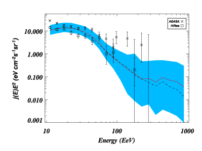
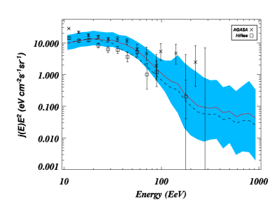
Figure 12: Energy spectra predicted for iron injection in the presence of the EGMF obtained from the LSS simulation. The average (solid line) and cosmic variance (shaded band) are obtained as in Figs. 3 and 7. The average source spectral index is $\langle\alpha\rangle=2.0$. The maximum injection energy is set to 4 ZeV (top panel) and 10 ZeV (bottom panel). The dashed lines represent average spectra in the case $\langle\alpha\rangle=2.4$.

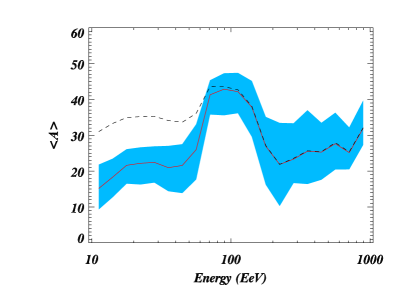
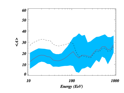
Figure 13: Predicted average atomic mass $\langle A\rangle$ as a function of observed particle energy corresponding to the spectra shown in Fig. 12 for iron injection in the presence of the EGMF. Mean and cosmic variance are computed as in Fig. 12 with $\langle\alpha\rangle=2.0$ and maximum injection energy of 4 ZeV (top panel) and 10 ZeV (bottom panel). The influence of the EGMF is apparent from comparing with Fig. 8 for the same case without EGMF. The dashed line corresponds to a mean injection spectrum $\langle\alpha\rangle=2.4$ instead of 2.

The spectra obtained in presence of magnetic deflections are presented in Fig. 12, and can be compared to Fig. 7. The bump which was predicted between 20 and 30 EeV without EGMF now appears as a smooth feature in a broader energy range, $10\lesssim E\lesssim 40\,$EeV. There is no steepening of the flux at 100 EeV, comparable to proton injection, and contrary to the case with no EGMF.

At higher energies, we observe a flattening of the spectrum as in the absence of EGMF. The flux is higher than without EGMF, at least statistically: For $E_{\rm max}=4$ ZeV, we predict $\langle JE^{2}\rangle\sim 0.1\,{\rm eV}\,{\rm cm}^{-2}\,{\rm s}^{-1}\,{\rm sr}^{-1}$ at $\sim 500$ EeV with EGMF, instead of $\sim 0.01\,{\rm eV}\,{\rm cm}^{-2}\,{\rm s}^{-1}\,{\rm sr}^{-1}$ in the absence of EGMF.

The average atomic mass $\langle A\rangle$ as a function of energy is presented in Fig. 13. At energies $E\lesssim 60\,$EeV, it can be seen that, depending on the average injection spectral index $\langle\alpha\rangle$, $\langle A\rangle\sim 15-30$ instead of $\langle A\rangle\sim 30-50$ in the absence of EGMF. The interpretation is that, as explained in Ref. bertone , magnetic fields increase the mean path length between sources and observer and the resulting increase in interactions also drives up the relative proportion of lighter secondaries to iron. As a consequence, it is very interesting to remark that a measured average mass of UHECRs at energies $10\lesssim E\lesssim 30\,$EeV larger than $\simeq 35$ would imply that deflections due to EGMF are relatively small, independently of the nature of particles accelerated at the source. This can be another test for extragalactic magnetic field effects, independently from anisotropy studies lss-protons . The trend of $\langle A\rangle$ with spectral index $\langle\alpha\rangle$ is the same as in the absence of EGMF. Furthermore, the shape of the mass distribution is similar to Fig. 9, except that abundances of light elements with $A\lesssim 6$ tend to be increased by a factor 2–3 which corresponds to the decrease in $\langle A\rangle$ seen in comparing Fig. 8 with Fig. 13.

At higher energies the energy dependence of $\langle A\rangle$ around $\sim 100\,$EeV depends crucially on the source parameters $E_{\rm max}$ and $\alpha$, as in the absence of EGMF. The EGMF can lead to additional modification of the composition, as seen by comparing Figs. 13 with 8.

V.2 Anisotropies: Deflections and Sky Maps

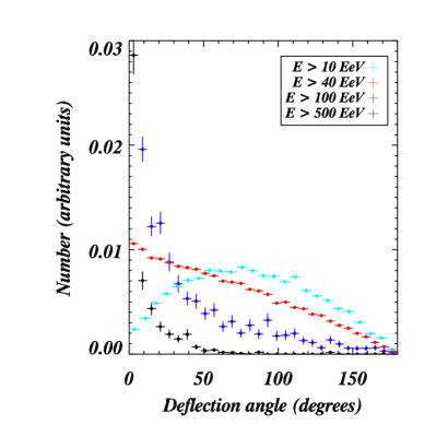
Figure 14: Histogram of deflection angles of observed UHECRs for different cuts in energy, in the case of iron injection with $\alpha=2$. As in Fig. 5, the distributions are cumulated over all source location realizations and the error bars are Poissonian, reflecting the finite number of simulated trajectories.

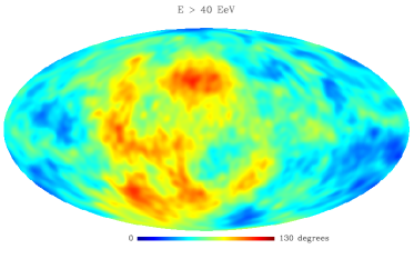
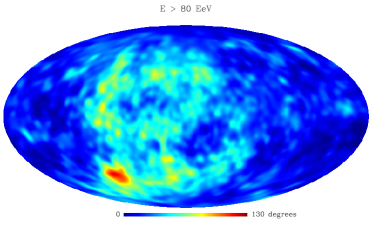
Figure 15: Sky distribution of deflections obtained from events recorded by the observer in the case of iron injection with EGMF, accumulated over all simulated realizations. Top panel: Events above 40 EeV. Bottom panel: Events above 80 EeV. The maps have been smoothed with beams of 5 degrees.

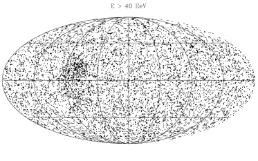
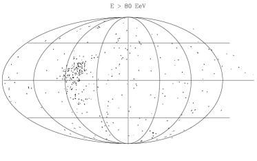
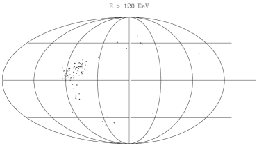
Figure 16: Example of arrival directions of events above 40, 80, and 120 EeV in a particular source realization, with roughly 150 events recorded above 100 EeV. In this realization, at high energy an individual source emerges progressively from the background.

As expected, the histogram of deflection angles for iron injection, presented in Fig. 14, shows typical deflections larger than for proton injection. This is particularly the case at the highest energies, since at those energies the observed particles are mostly heavy nuclei, whose local deflection is therefore up to 56 times larger than in the case of protons. As a result, typical deflections of $10^{\circ}$ or more are expected even at 500 EeV.

Sky distributions of deflection angles in the framework of this scenario are presented in Fig. 15 for energies above 40 and 80 EeV. The considerable inhomogeneity of these maps reflects the presence of extended magnetized structures distributed along the LSS. There is a striking difference between these maps and the one presented in Ref. dolag : Even at 80 EeV, there is still a large part of the sky where deflections are typically $\geq 50^{\circ}$. This is due to at least two reasons: Apart from the larger charge of the UHECRs in this scenario, the EGMF in our simulation is more extended, as discussed previously.

These deflections may prevent us from performing straightforward “UHECR astronomy” with forecoming experiments such as the Pierre Auger Observatories. However, they do not erase all the structures in the sky either, and in particular the expected low source density may allow to identify extended sources in the sky even within this unfavorable scenario. An example is given in Fig. 16, where arrival direction maps are represented for a given source realization with iron injection and EGMF, and a statistics of $\simeq 150$ recorded trajectories above $10^{20}$ eV. At 40 EeV, the sky is dominated by an isotropic cosmological background, but at higher energies the background disappears and a small number of nearby sources emerge. These sources are clearly visible although they are not point-like. It has to be noticed that, if such a configuration were realized in nature, then the very few sources one expects to contribute at the highest energies can be found in the northern hemisphere, where Virgo is located, emphasizing the need for a northern UHECR observatory.

V.3 Anisotropies: Auto-Correlation and Angular Power Spectrum

V.3.1 Auto-Correlation Function

Figure 17: Auto-correlation function for events above 40, 80 and 120 EeV in the case of iron injection with EGMF. We do not show the auto-correlation in the first bin and showers have been corrected for. The error bars represent the cosmic variance, computed in the same way as for spectra and composition: Various source location configurations are considered, and for each one 50 source intensity and spectral indexes are drawn. ${\cal N}(\theta)=1$ corresponds to isotropy.

The large deflections do not prevent us from observing a strong auto-correlation signal at high energies, due to the low source density. We present in Fig. 17 the auto-correlation predicted for this scenario, computed with a 1 degree binning. Due to the computational reasons discussed in Sect. II, we count nuclei showers as only one particle and we disregard the first angular bin. It can be seen that above 40 EeV, the predicted auto-correlation signal is almost flat, whereas above 80 EeV it reaches a factor $\sim 4$ above the isotropic level, and much larger values above 120 EeV. Fig. 17 also shows that the predicted auto-correlation signal is highly dependent on the source configuration, and can extend over 10 degrees or more due to diffusion in the EGMF.

When comparing Fig. 17 to Fig. 11, it can be seen that the effect of magnetic fields is to strongly reduce the intensity of the auto-correlation peak at small angles: at 80 EeV, the reduction factor is $\sim 10$. Due to the larger deflection of nuclei this suppression is stronger than for protons.

We remark that the galactic magnetic fields, which were not take into account here, will also increase this smoothing of auto-correlation over larger angular scales.

V.3.2 Angular Power Spectrum

Figure 18: Example of predicted angular power spectra for two source configurations for the scenario with iron injection and EGMF. Top panel: Events with $E\geq 40\,$EeV; the corresponding event map is roughly isotropic and contains several thousand events. With reweighting, we predict $\left<C_{\ell}\right>=1.54\times 10^{-4}$, i.e. $N_{\rm eff}\simeq 500$ effective events, see Eq. (3); this level is indicated by the dashed line. Bottom panel: Events with $E\geq 120\,$EeV. Two nearby sources appear in the corresponding map. The average $\left<C_{\ell}\right>$ predicted from isotropy is $7.1\times 10^{-3}$ (dashed line), and the average $\left<C_{\ell}\right>$ predicted by the simulation implies $N_{v}=2.2$ “effective point sources”. Furthermore, $C_{\ell}$ decreases with increasing $l$, which reflects the spatial extension of the sources.

Figure 19: Angular power spectra for events above 40, 80 and 120 EeV in the case of iron injection with EGMF. The error bars represent the cosmic variance computed in the same way as in Fig. 17. The dashed line corresponds to an isotropic distribution of the same number of $10^{4}$ simulated, weighted events above 40 EeV.

In Figs. 18 and 19, we present examples of angular power spectra, and their averages and fluctuations for given energy thresholds. The predictions are similar to those obtained in the absence of EGMF in Fig. 10. The theoretical prediction for the power spectrum in the isotropic case is given by the expressions in Eq. (3). As the large fluctuations show, the power spectrum depends on the energy threshold, as well as on the source configuration.

Above 40 EeV the mean angular power spectrum is almost flat and consistent with predictions from isotropy; however some realizations exhibit some large-scale patterns visible in the low-order $C_{\ell}$. When increasing the energy, the angular power spectrum remains roughly flat, but at levels much higher than expected from isotropy. Indeed, at high energies there is only a small number $N_{v}$ of bright sources visible in any given realization, leading to a mean value of $C_{\ell}=(4\pi N_{v})^{-1}$. The power spectrum is then approximatively flat, with deviations from flatness caused by the observed source extension due to deflection in the EGMF. Above 80 EeV, the average $\langle C_{\ell}\rangle$ is $5\times 10^{-3}$, leading to an average value $N_{v}\simeq 16$ visible sources, whereas above 120 EeV we have $\left<C_{\ell}\right>\sim 0.03$, and therefore, only 2.7 sources are visible on average.

The angular power spectrum is a useful tool to estimate the effective number of observed sources above a given energy, but otherwise it appears to be of quite limited use within the scenario under consideration: At energies below 40 EeV, deflections are too large to expect a large-scale signal, and at high energies the large values predicted for $C_{\ell}$ are only due to the finite number of visible sources.

V.3.3 Detection with Finite Statistics

When comparing predictions of auto-correlations and power spectra such as shown in Figs. 17–19 with future data, one has to take into account also the statistical error due to the finite number $N_{\rm obs}$ of the actually observed events. This has not been included in Figs. 17–19 which thus correspond to $N_{\rm obs}\rightarrow\infty$. The error bars due to finite statistics can be assigned directly to the observational angular power spectra or auto-correlations, as these errors depend on the detector aperture.

In the same way, we have not taken into account the detector exposure in our anisotropy predictions, as it can be taken into account directly in the experimental data.

Alternatively, the finite number of experimental events and non-trivial exposure functions as well as angular and energy resolutions can be assigned to the predictions by drawing mock data sets from maps constructed from the simulated trajectories, as done in Ref. lss-protons .

However, we can roughly estimate the number of events needed in the case of uniform exposure to detect the anisotropies predicted in our model. This can be done by estimating the error due to the finite number of events and requiring it to be smaller than cosmic variance and/or the deviation from predictions based on isotropy.

Even in the case of partial sky coverage, the statistical error on the angular power spectrum estimation has been computed deligny , but the isotropic formula $\sigma(C_{\ell})\sim C_{\ell}\simeq 1/(4\pi N_{\rm obs})$ ($C_{\ell}$ is a quadratic estimator), at low $\ell$, is sufficient for our purposes. From Fig. 19, we predict $C_{\ell}\sim 0.005$ above 80 EeV. Requiring $\sigma(C_{\ell})\sim 0.001$ for a detection implies to have $N_{\rm obs}\gtrsim 80$ events above $8\times 10^{19}$ eV, which has not been yet reached by AGASA, but will be easily reached by the Pierre Auger project.

As for the auto-correlation function ${\cal N}(\theta)$, we predict an excess $\cal N$ $\sim 4$ for $\theta\lesssim\theta_{0}=2^{\circ}$ at 80 EeV, see Fig. 17. For $N_{\rm obs}$ events, the Poissonian error on $\cal N$ is $\sigma({\cal N})\simeq(N_{\rm obs}^{2}\theta_{0}^{2}/4)^{-1/2}$. Requiring $\sigma({\cal N})\leq 0.8$ for a detection leads to $N_{\rm obs}\gtrsim 70$ events needed above $8\times 10^{19}$ eV.

Overall, the anisotropies arising in the framework of this model are largely detectable by the Pierre Auger Observatory.

VI Conclusions

We performed numerical simulations of ultrahigh energy nuclei propagation in a structured, magnetized universe. The sources, of density $\sim 10^{-5}\mbox{Mpc}^{-3}$, were distributed proportionally to the baryon density obtained from the large scale structure simulation of Ref miniati . We considered either negligible magnetic fields or fields obtained from that same simulation of large scale structure formation and seeded by the Biermann battery around cosmic shocks. Their strength has been normalized to $\sim\mu$G in the core of the most prominent simulated collapsed structure lss-protons . We injected iron and protons at the sources, and in the case of iron we followed all secondary nuclei produced by photo-disintegration.

Below the GZK feature, protons tend to dominate the spectrum even for exclusive iron injection, due to photo-disintegration of high-energy heavy nuclei. However, the predicted spectrum does not match the observations by AGASA and HiRes at these energies, and a light component from injection of light nuclei or protons must contribute to the spectrum at sub-GZK energies.

Above $\simeq 30\,$EeV existing data are poor and consistent with an UHECR flux exclusively resulting from iron injection. As the maximum energy reachable with shock acceleration increases with the charge of the nucleus, it makes sense to expect a heavy nuclei component above the GZK energy. Within our scenario we found the following generic predictions in the case of pure iron injection:

• The average mass $\langle A\rangle$ of observed particles strongly depends on the scenario and typically is $\sim 20-30$ above $\simeq 100$ EeV. If $\langle A\rangle\gtrsim 35$ is observed at energies below 30 EeV, the effect of extra-galactic magnetic fields on propagation cannot be too strong since it would increase photo-disintegration. Below $\simeq 100\,$EeV, $\langle A\rangle$ increases with increasingly steeper injection spectrum.

• If some sources are located within a few Mpc from the observer, a flattening of the spectrum after the GZK feature results. This flattening is more pronounced than in the case of proton primaries, but cosmic variance is much larger as well. When the spectrum is normalized around 30 EeV, the flattening tends to be stronger for significant EGMF.

• A low source density and considerable magnetic fields, especially around the sources, predict a significant clustering of UHECRs at super-GZK energies, typically on scales of order of the angular size of the magnetized region around the sources. In our simulation it is of order $\sim 10^{\circ}$. This can be seen from both auto-correlation function and angular power spectrum measurements at various energies.

• The injection spectra which allow to fit the observed spectra tend to be somewhat harder than in the case of protons, and cover the range $2.0\lesssim\alpha\lesssim 2.4$, but still consistent with expectations from theory of shock acceleration shock-acc .

The main feature of these simulations compared to previous work is the distribution of structured magnetic fields, compatible with existing data on extragalactic fields. These fields increase the deflection of nuclei, and, as a consequence, smooth the GZK feature in the energy spectrum as well as the auto-correlation signal at small angles. We also found that, for iron injection, there is a major cosmic variance at the highest energies for observables such as energy spectrum, composition and angular distribution, mostly due to the uncertainties in the location of the sources.

At the highest energies the observed flux will be dominated by only a few sources within the GZK-distance, $\simeq 50\,$Mpc, from the observer. Although extra-galactic magnetic fields can considerably smear out the images of the sources, their location may still be determined by next generation experiments to within $10-20^{\circ}$.

In the presence of EGMF auto-correlations are reduced by factors of order 10, and thus more strongly than in the case of proton injection lss-protons . However, even in the presence of the relatively strong EGMF considered in the present work, auto-correlations remain significant. As a consequence, if no auto-correlation is observed, the source density must be larger than $10^{-5}\mbox{Mpc}^{-5}$. Recall that this density is motivated by the claimed AGASA clustering blasi ; kachelriess .

We have now explored an extensive series of plausible scenarios in the context of an astrophysical UHECR origin. The scenario mostly studied here, because of the large magnetic fields involved over extended regions, of the small source density compared to interaction lengths, and of the fact that we inject iron nuclei at the sources, appears to be the “worst case” in terms of fluctuations of the predictions of observables. Hopefully, the Pierre Auger Observatory will soon allow to select a specific scenario if its data is compatible with an astrophysical origin of UHECRs.

References

- (1) J. W. Cronin, arXiv:astro-ph/0402487.
- (2) The Pierre Auger Observatory Design Report (ed. 2), March 1997; see also http://www.auger.org.
- (3) M. Takeda et al., Phys. Rev. Lett. 81, 1163 (1998) [arXiv:astro-ph/9807193].
- (4) A. Zech, arXiv:astro-ph/0409140.
- (5) K. Shinozaki et al., Astrophys. J. 571, L117 (2002).
- (6) A. A. Watson, arXiv:astro-ph/0408110.
- (7) M. Takeda et al., Astrophys. J. 522, 225 (1999) [arXiv:astro-ph/9902239];
- (8) C. B. Finley and S. Westerhoff, Astropart. Phys. 21, 359 (2004) [arXiv:astro-ph/0309159].
- (9) S. Westerhoff [The High Resolution Fly’s Eye Collaboration], arXiv:astro-ph/0408343.
- (10) for a review see, e.g., P. Bhattacharjee and G. Sigl, Phys. Rept. 327, 109 (2000) [arXiv:astro-ph/9811011].
- (11) K. Greisen, Phys. Rev. Lett. 16, 748 (1966); G. T. Zatsepin and V. A. Kuzmin, JETP Lett. 4, 78 (1966) [Pisma Zh. Eksp. Teor. Fiz. 4, 114 (1966)].
- (12) D. F. Torres and L. A. Anchordoqui, Rept. Prog. Phys. 67, 1663 (2004) [arXiv:astro-ph/0402371].
- (13) see, e.g., J. P. Vallée, New Astrn. Reviews 48, 763 (2004).
- (14) G. Sigl, F. Miniati and T. A. Ensslin, Phys. Rev. D 70, 043007 (2004) [arXiv:astro-ph/0401084].
- (15) G. Sigl, F. Miniati and T. Ensslin, arXiv:astro-ph/0409098.
- (16) K. Dolag, D. Grasso, V. Springel and I. Tkachev, JETP Lett. 79, 583 (2004) [Pisma Zh. Eksp. Teor. Fiz. 79, 719 (2004)] [arXiv:astro-ph/0310902]; K. Dolag, D. Grasso, V. Springel and I. Tkachev, arXiv:astro-ph/0410419.
- (17) A. M. Hillas, Ann. Rev. Astron. Astrophys. 22, 425 (1984).
- (18) J. L. Puget, F. W. Stecker and J. H. Bredekamp, Astrophys. J. 205, 638 (1976); L. N. Epele and E. Roulet, Phys. Rev. Lett. 81, 3295 (1998) [arXiv:astro-ph/9806251]; L. N. Epele and E. Roulet, JHEP 9810, 009 (1998) [arXiv:astro-ph/9808104]; F. W. Stecker, Phys. Rev. Lett. 81, 3296 (1998); F. W. Stecker and M. H. Salamon, Astrophys. J. 512, 521 (1992) [arXiv:astro-ph/9808110].
- (19) G. Bertone, C. Isola, M. Lemoine and G. Sigl, Phys. Rev. D 66, 103003 (2002) [arXiv:astro-ph/0209192].
- (20) T. Yamamoto, K. Mase, M. Takeda, N. Sakaki and M. Teshima, Astropart. Phys. 20, 405 (2004) [arXiv:astro-ph/0312275].
- (21) G. Sigl, JCAP 0408, 012 (2004) [arXiv:astro-ph/0405549].
- (22) F. Miniati, Mon. Not. Roy. Astron. Soc. 337, 199 (2002) [arXiv:astro-ph/0203014].
- (23) R. Aloisio and V. Berezinsky, arXiv:astro-ph/0403095.
- (24) P. Blasi and D. De Marco, Astropart. Phys. 20, 559 (2004) [arXiv:astro-ph/0307067].
- (25) M. Kachelriess and D. Semikoz, arXiv:astro-ph/0405258.
- (26) H. Yoshiguchi, S. Nagataki and K. Sato, Astrophys. J. 596, 1044 (2003) [arXiv:astro-ph/0307038].
- (27) E. Weibel, Phys. Rev. Lett. 2, 83 (1959).
- (28) L. O. Silva, R. A. Fonseca, J. Tonge, J. M. Dawson, W. B. Mori and M. V. Medvedev, Astrophys. J. 596, L121 (2003) [arXiv:astro-ph/0307500].
- (29) R. Schlickeiser and P. K. Shukla, Astrophys. J. 599, L57 (2003).
- (30) D. Ryu, H. Kang, and P. L. Biermann, Astron. Astrophys. 335 (1998) 19.
- (31) T. E. Clarke, P. P. Kronberg and H. Boehringer, Astrophys. J. 547, L111 (2003) [arXiv:astro-ph/0011281].
- (32) M. Johnston-Hollitt and R. D. Ekers, arXiv:astro-ph/0411045.
- (33) O. Deligny et al., JCAP 0410, 008 (2004) [arXiv:astro-ph/0404253].
- (34) see, e.g., D. C. Ellison and G. P. Double, Astropart. Phys. 22, 323 (2004) [arXiv:astro-ph/0408527].
- (35) see http://www.eso.org/science/healpix/.