Highly Ionized Gas in the Galactic Halo and the High Velocity Clouds Toward PG 1116+215

Abstract

We have obtained high resolution FUSE and HST/STIS echelle observations of the quasar PG $1116+215$ ($z_{\mathrm{em}}=0.1765$, $l=223\fdg 36$, $b=+68\fdg 21$). The semi-continuous coverage of the ultraviolet spectrum over the wavelength range 916–2800 Å provides detections of Galactic and high velocity cloud (HVC) absorption over a wide range of ionization species: H I, C II-IV, N I-II, O I, O VI, Mg II, Si II-IV, P II, S II, and Fe II over the velocity range $-100<v_{\mathrm{LSR}}<+200$ km s^-1. The high dispersion of these spectra (6.5-20 km s^-1) reveals that low ionization species consist of five discrete components: three at low- and intermediate-velocities ($v_{\mathrm{LSR}}\approx-44,-7,+56$ km s^-1), and two at high velocities ($v_{\mathrm{LSR}}\approx+100,+184$ km s^-1). Over the same velocity range, the higher ionization species (C III-IV, O VI, Si IV) - those with ionization potentials larger than 40 eV - show continuous absorption with column density peaks at $v_{\mathrm{LSR}}\approx 10$ km s^-1, the expected velocity of halo gas co-rotating with the Galactic disk, and $v_{\mathrm{LSR}}\approx+184$ km s^-1, the velocity of the higher velocity HVC. The velocity coincidence of both low and high ionization species in the $v_{\mathrm{LSR}}\approx+184$ km s^-1 HVC gas suggests that they arise in a common structure, though not necessarily in the same gaseous phase. The absorption structure in the high ionization gas, which extends to very low velocities, suggests a scenario in which a moderately dense cloud of gas is streaming away from the Galaxy through a hot external medium (either the Galactic halo or corona) that is stripping gas from this cloud. The cloud core produces the observed neutral atoms and low-ionization species. The stripped material is the likely source of the high-ionization species. Among the host of collisionally-ionized non-equilibrium models, we find that shock-ionization and conductive interfaces can account for the column density ratios of high ionization species. The nominal metallicity of the neutral gas, using the O I and H I column densities is $[$O/H$]\sim-0.66$, with a substantial uncertainty due to the saturation of the H I Lyman series in the FUSE band. The ionization of the cloud core is likely dominated by photons, and assuming the source of ionizing photons is the extragalactic UV background, we estimate the cloud has a density of $10^{-2.7}$ cm^-3 with a thermal pressure $p/k\approx 24$ cm^-3 K. If photons escaping the Galactic disk are also included (i.e., if the cloud lies closer than the outer halo), the density and thermal pressure could be higher by as much as 2 dex. In either case, the relative abundances of O, Si, and Fe in the cloud core are readily explained without departures from the solar pattern. We compare the column density ratios of the HVCs toward the PG $1116+215$ to other isolated HVCs as well as Complex C. Magellanic Stream gas (either a diffuse extension of the leading arm or gas stripped from a prior passage) is a possible origin for this gas and is consistent with the location of the high velocity gas on the sky, as well as its high positive velocity, the ionization, and metallicity.

1 Introduction

Recent observations with the Far Ultraviolet Spectroscopic Explorer (FUSE) have revealed a complex network of highly-ionized high-velocity gas in the vicinity of the Galaxy. This new information demonstrates that the high-velocity material is far more complex than originally thought and is providing new insight into the formation and evolution of the Milky Way. The primary diagnostic of this gas is the O VI$\lambda 1031.926$ line, which is seen in absorption at velocities exceeding $\sim 100$ km s^-1 in the Local Standard of Rest in at least 60% of the AGN/QSO sight lines observed in the first few years of FUSE operations (Wakker et al., 2003). Sembach et al. (2003) have attributed the high velocity O VI to collisionally ionized gas at the boundaries between warm circumgalactic clouds and a highly extended ($R\gtrsim 70$ kpc), hot ($T>10^{6}$ K), low-density ($n\lesssim 10^{-4}$ cm^-3) Galactic corona or Local Group medium. This result is supported by detailed investigations of the relationship between the highly ionized gas and lower ionization species (e.g., C II, C IV, Si II-IV) in high velocity cloud Complex C (Fox et al., 2004) and the high velocity clouds (HVCs) along the sight line toward PKS 2155-304 (Sembach et al., 1999; Collins, Shull, & Giroux, 2004b). An alternate explanation for the origin of the high velocity O VI – photoionization in a low density plasma – has also been considered (Nicastro et al., 2002) but is difficult to reconcile with data available for the other O VI HVCs (Sembach et al., 2004b; Collins et al., 2004b).

Establishing the relationship of the high velocity O VI with lower ionization gas and pinpointing its possible origins requires high-resolution observations of other ionization stages with the Hubble Space Telescope (HST). We have obtained Space Telescope Imaging Spectrograph (STIS) observations of the bright quasar PG 1116+215 ($l=223\fdg 36$, $b=+68\fdg 21$, $m_{\rm{}_{V}}\approx 15.2$, $z_{\mathrm{em}}=0.1765$) to study the high velocity O VI in a direction that is well away from large concentrations of high velocity H I observable in 21 cm emission (e.g., the Magellanic Stream, Complexes A, C, M). High velocity gas in this sight line was first noted by Tripp, Lu, & Savage (1998), using HST observations with the Goddard High Resolution Spectrograph. The sight line contains high velocity O VI at $v_{\mathrm{LSR}}\approx+184$ km s^-1 (Sembach et al., 2003). High velocity gas in this general region of the sky is often purported to be extragalactic in nature based upon its kinematical properties (Blitz et al., 1999; Nicastro et al., 2003, – but see Wakker (2004b) for a rebuttal to these arguments). PG 1116+215 is on the opposite side of the sky from the PKS 2155-304 and Mrk 509 sight lines, which are the only other isolated HVCs to have had their ionization properties studied in detail. It therefore presents an excellent case to test whether the ionization and kinematical properties of the O VI and other ionization stages are consistent with an extragalactic location. The sight line passes through the hot gas of the Galactic halo as well as several intermediate-velocity clouds located within a few kiloparsecs of the Galactic disk (e.g., Wakker, 2004a, and references therein). Thus, observations of this single sight line also provide self-contained absorption fiducials against which to judge the character of the high-velocity absorption.

A complete spectral catalog of the FUSE and STIS observations for the PG 1116+215 sight line is presented in a companion study by Sembach et al. (2004a). Information about the intergalactic absorption-line systems along the PG 1116+215 sight line can be found in that paper. In §2, we present the spectroscopic data available for the Galactic and high velocity absorption in the sight line. In §3, we provide a general overview of the absorption profiles and make preliminary assessments of the kinematics of the Galactic absorption and the high velocity gas. In §4, we describe our methodology for line measurements (e.g., equivalent widths, column densities) and present these for selected regions of the absorption profiles. In addition, we present composite apparent column density profiles for a sample of important species. In the following sections, we discuss and analyze the Galactic and intermediate velocity absorption (§5), the high velocity absorption at $v_{\mathrm{LSR}}\approx 100$ km s^-1 (§6), and the high velocity absorption at $v_{\mathrm{LSR}}\approx 184$ km s^-1 (§7). Finally, we discuss the implications of this study and summarize our findings in §8 and §9, respectively.

2 Observations & Data Processing

We observed PG $1116+215$ with FUSE on two separate occasions in April 2000 and April 2001. For all observations PG $1116+215$ was aligned in the center of the LiF1 channel LWRS ($30\arcsec\times 30\arcsec$) aperture used for guiding. The remaining channels (SiC1, SiC2, and LiF2) were co-aligned throughout the observations. The total exposure time was 77 ksec in the LiF channels and 64 ksec in the SiC channels after screening the time-tagged photon event lists for valid data. We processed the FUSE data with a customized version of the standard FUSE pipeline software (CALFUSE v2.2.2). The data have continuum signal-to-noise ratios $S/N\sim 18$ and 14 per 0.07 Å (20–22 km s^-1) spectral resolution element in the LiF1 and LiF2 channels at 1050 Å, and $S/N\sim 8$ and 13 at 950 Å in the SiC1 and SiC2 channels. The zero-point velocity uncertainty and cross-channel relative velocity uncertainties are roughly 5 km s^-1. Further information about the acquisition and processing of the FUSE data can be found in Sembach et al. (2004a). A description of FUSE and its on-orbit performance can be found in articles by Moos et al. (2000) and Sahnow et al. (2000).

We observed PG $1116+215$ with HST/STIS in May-June 2000 with the E140M grating and $0.2\arcsec\times 0.06\arcsec$ slit for an exposure time of 20 ksec. We also obtained 5.6 ksec of E230M data through the $0.2\arcsec\times 0.09\arcsec$ slit. We followed the standard data reduction and calibration procedures used in our previous STIS investigations (see Tripp et al., 2001; Sembach et al., 2004a). The STIS data have a spectral resolution of 6.5 km s^-1 (FWHM) for the E140M grating, and 10 km s^-1 (FWHM) for the E230M grating, both with a sampling of 2–3 pixels per resolution element. The zero-point heliocentric velocity uncertainty is about 0.5 pixels, or $\sim 1.5$ km s^-1 for E140M, and $\sim 2.5$ km s^-1 for E230M (Proffitt et al., 2002). The E140M spectra have $S/N\approx 14-15$ per resolution element at 1300 Å and 1500 Å. The E230M spectra have $S/N\approx 6.6-8$ per resolution element at 2400 Å and 2800 Å. For additional information about STIS, see Woodgate et al. (1998), Kimble et al. (1998), and Proffitt et al. (2002). We plot sample FUSE and STIS spectra in Figure 1. The three panels are scaled to cover the same total velocity extent. Interstellar absorption features are labelled, and high velocity lines are indicated with offset tick marks.

We identified Galactic absorption features that were detected at $\geq 3\sigma$ confidence using the method from Schneider et al. (1993), with atomic data from Morton (2003). In Figures 2a-f, we show velocity-stacked flux profiles in the Local Standard of Rest (LSR) for the metal-line transitions detected in Galactic absorption. The dashed vertical lines at 100 km s^-1 and 184 km s^-1 in each panel mark the locations of the high velocity absorption. The panels are ordered by atomic number and ionization stage of the absorbing species. The detected transitions range over a decade in ionization potential from $\sim 1-10$ Rydbergs.

3 A General Tour Of the Absorption

The sight line toward PG $1116+215$ lies at high Galactic latitude, $l=223\fdg 36$ and $b=+68\fdg 21$, where the transformation from heliocentric velocity to Local Standard of Rest velocity is small. Using the Mihalas & Binney (1981) definition for the Local Standard of Rest, and canonical values for standard Solar motion, we find $v_{\mathrm{LSR}}=v_{\mathrm{helio}}+1.0$ km s^-1. (The correction in transforming heliocentric velocities to Local Standard of Rest velocity is $v_{\mathrm{LSR}}=v_{\mathrm{helio}}+0.6$ km s^-1, if one uses the conventions adopted by IAU Commission 33.) Wakker et al. (2003) present an H I 21 cm emission profile and report components at $v_{\mathrm{LSR}}=-42$ km s^-1, which they identify with the S1 clump of the Intermediate Velocity-Spur, and at $v_{\mathrm{LSR}}=-7$ km s^-1. For the centroid velocity of the Intermediate-Velocity Spur, Sembach et al. (2004a) report a velocity of $v_{\mathrm{LSR}}=-44$ km s^-1 using unsaturated lines from low-ionization species and H₂. We adopt the Sembach et al. (2004a) velocity in our analysis. As pointed out by Kuntz & Danly (1996), $v_{\mathrm{LSR}}<0$ intermediate velocity gas in this direction is inconsistent with pure Galactic rotation, and likely originates from either infalling gas, turbulent clouds, or a Galactic fountain. A simple model of uniform density, non-turbulent co-rotating gas within 10 kpc of the disk would produce absorption in the velocity range $0\lesssim v_{\mathrm{LSR}}\lesssim 15$ km s^-1.

The two velocity components detected in H I 21 cm emission by Wakker et al. (2003) are readily visible at $v_{\mathrm{LSR}}\lesssim 10$ km s^-1 in the low-ionization species like S II, which do not suffer from unresolved saturated structure. In most neutral and low-ionization species, however, these two components are strongly saturated and blended together. At larger velocities ($10\lesssim v_{\mathrm{LSR}}\lesssim 100$ km s^-1), there is an additional intermediate velocity component in the low ionization species at $v_{\mathrm{LSR}}\approx 56$ km s^-1, which is not detected in the H I 21 cm emission [down to $N$(H I)$\sim 2\times 10^{18}$ cm^-2]. (Absorption at this velocity is evident in the H I Lyman series, which we treat later.) This intermediate velocity component is readily apparent in the strong lines of neutral (e.g., O I) and low-ionization (e.g., Mg II, Si II, Fe II) species.

At velocities exceeding $|v_{\mathrm{LSR}}|=100$ km s^-1, there are two absorption components, at $v_{\mathrm{LSR}}\approx+100$ km s^-1 and $v_{\mathrm{LSR}}\approx+184$ km s^-1. The $v_{\mathrm{LSR}}\approx+100$ km s^-1 absorption component is prominent in the C II and Si III profiles, but noticeably absent in other low-ionization (e.g., Mg II, Fe II) and neutral (e.g., O I) species. The component is detected (at $3\sigma$ confidence) in the strongest Si II line at 1260.422 Å, but not in the weaker lines. Absorption at this velocity is also detected in other moderate-ionization species (C III) as well as high ionization-species (C IV, Si IV, O VI). The HVC at $v_{\mathrm{LSR}}\approx+184$ km s^-1 is detected in a wide range of neutral (O I), low-ionization (C II, N II, Mg II, Si II, Fe II), moderate-ionization (C III, Si III), and high-ionization (C IV, Si IV, O VI) species.

In Figure 2 there are noticeable differences in the kinematics of the high and low ionization species. The neutral and low-ionization species typically break up into discrete components (when the lines are not too strong) at the five velocities discussed ($v_{\mathrm{LSR}}\approx-44,-7,+56,+100,+184$ km s^-1). By contrast, the higher ionization species (C III, C IV, O VI, Si IV) feature continuous absorption across the entire low, intermediate, and high velocity range. The kinematic distributions of these higher ions have an apparent bimodality, with apparent optical depth peaks defining the low velocity Galactic absorption and the high velocity absorption. The fluxes do not return to the continuum level in between these absorbing zones except for Si IV which may be due to (1) the lower elemental abundance of silicon compared to carbon and oxygen, and (2) the lower ionization of Si IV relative to C IV and O VI. It is interesting to note, however, that at low velocity the flux minimum of the O VI profile does not coincide with the negative velocity component seen in Si IV and C IV (the intermediate velocity S1 component at $v_{\mathrm{LSR}}\approx-44$ km s^-1), but rather the expected location for Galactic halo absorption, $v_{\mathrm{LSR}}\sim 10$ km s^-1. At the velocity of the higher velocity HVC ($v_{\mathrm{LSR}}\approx+184$ km s^-1), the high-ionization species coincide with the lower ionization species. This velocity coincidence suggests that high and low ionization absorption arise co-spatially in that component. However, there are noticeable differences, as already mentioned, in the general shapes of the high and low ionization species, indicating absorption from a common structure with different phases.

4 Measurements

We use apparent optical depth (AOD) techniques described by Sembach & Savage (1992) to measure equivalent widths, integrated apparent column densities, velocity centroids, and $b$-values for the five components discussed above. Using the low and moderate-ionization species (primarily S II, Fe II, and Si III) as guides, we chose the following integration ranges for the five components: $-100\leq v_{\mathrm{LSR}}\leq-25$ km s^-1 for $v_{\mathrm{LSR}}\approx-44$ km s^-1; $-25\leq v_{\mathrm{LSR}}\leq+37$ km s^-1 for $v_{\mathrm{LSR}}\approx-7$ km s^-1; $+37\leq v_{\mathrm{LSR}}\leq+85$ km s^-1 for $v_{\mathrm{LSR}}\approx+56$ km s^-1; $+85\leq v_{\mathrm{LSR}}\leq+140$ km s^-1 for $v_{\mathrm{LSR}}\approx+100$ km s^-1; and $+140\leq v_{\mathrm{LSR}}\leq+230$ km s^-1 for $v_{\mathrm{LSR}}\approx+184$ km s^-1.

We first extracted a $\pm 500$ km s^-1 window about the rest wavelength of each line into separate files. We then determined a local continuum for each line following the Legendre polynomial-fitting method described by Sembach & Savage (1992). We computed the equivalent width of each transition of rest wavelength $\lambda_{\circ}$ for the two high velocity clouds and for the Galactic/IVC absorption by performing the sum:

$$W_{\lambda}={\lambda_{\circ}\over c}\sum_{i=i_{\mathrm{min}}}^{i_{\mathrm{max}}}w_{i}[1-I(v_{i})]\delta v_{i},$$ (1)

where the limits of the sum ($i_{\mathrm{min}}$ and $i_{\mathrm{max}}$) were chosen to encompass the specified velocity range for the component, $\delta v_{i}=v_{i+{1\over 2}}-v_{i-{1\over 2}}$ is the full width of a bin, $I(v_{i})$ is the normalized flux profile as a function of velocity, and $w_{i}$ is a weight that accounts for the fractional bins at the edges of the summation.

The integrated apparent column density, AOD-weighted centroid velocity, and $b$-value are all derived as moments of the apparent optical depth distribution. To compute these quantities, we first transform the normalized flux profiles to apparent column density (ACD) profiles via:

$$N_{\mathrm{a}}(v_{i})={{m_{\mathrm{e}}c}\over{\pi e^{2}}}{1\over{f\lambda_{\circ}}}\ln\left[{1\over{I(v_{i})}}\right],$$ (2)

where $f$ is the oscillator strength of the transition. From the ACD profiles, the desired quantities are computed via:

$$N_{\mathrm{a}}^{(j)}=\sum_{i=i_{\mathrm{min}}}^{i_{\mathrm{max}}}w_{i}v^{j}N_{\mathrm{a}}(v_{i})\delta v_{i}$$ (3)

$$N_{\mathrm{a}}=N_{\mathrm{a}}^{(0)}$$

$$\langle v\rangle=N_{\mathrm{a}}^{(1)}/N_{\mathrm{a}}^{(0)}$$

$$b^{2}=2\times N_{\mathrm{a}}^{(2)}/N_{\mathrm{a}}^{(0)}.$$

In the integrations involving moments of the apparent column density for strongly saturated lines, we treat pixels with negative flux (due to statistics) as having the flux equal to the RMS uncertainty derived from the fit to the continuum regions adjoining the line. We note that this causes the derived $N_{\mathrm{a}}(v)$ to be smaller than the true $N_{\mathrm{a}}(v)$ (see eq. 2) and the derived values of $N_{\mathrm{a}}$, $\langle v\rangle$, and $b$ will also be affected (see eq. 3). All other pixels are treated in the normal way, including those with fluxes above the continuum level where the implied apparent column density is negative. Since the moments of the optical depth for weak/narrow features are very sensitive to the choice of integration range, we only report mean velocities and $b$-values for lines whose equivalent width exceeds five times its $1\sigma$ error.

In Tables 1–2, we report measurements of the two high velocity components for the observed transitions of various species. In each table, we list the ion (column 1), transition rest wavelength (column 2), transition strength ($\log f\lambda$, column 3), centroid velocity (column 4), $b$-value (column 5), integrated apparent column density (column 6), equivalent width (column 7), and integration range (column 8) used to compute the aforementioned quantities. The errors quoted for each quantity are $1\sigma$ confidence errors resulting from both Poisson noise and continuum placement uncertainties. We also quote an additional error for the integrated column density and equivalent width which characterizes the systematic uncertainties based on our choice of integration range. This latter error is derived by splitting the difference between the addition and subtraction of 10 km s^-1 to the integration range (5 km s^-1 on either side of the range). In Table 3, we provide the same measurements for the the Galactic halo and intermediate velocity gas (integrating over the velocity range -100 to +85 km s^-1).

In Figure 3, we show the apparent column density profiles constructed using equation 2. For ions with more than one transition detected, we have over-plotted the apparent column density profiles. Apparent column density profiles from multiple transitions of a given species provide a means of testing for unresolved saturated structure, unidentified blends, and unocculted flux (e.g., scattered light within the instrument, or elevated background levels). In Table 4, we report our adopted column densities for the five absorption components. These column densities were derived by computing the variance-weighted mean of the integrated column densities of transitions least affected by unresolved saturated structure or other peculiarities. In the appendix, we provide a detailed description of the transitions covered for each ion, and discuss which transitions were used in the computations of the composite apparent column density profiles and the adopted column densities.

In cases where multiple transitions from a given species exist, we compute composite apparent column density profiles in order to improve the data quality and maximize use of the available information in a non-parametric way. Comparisons of these profiles allows inspection of the kinematical similarities/differences that exist between different species. Using the composite profile information also avoids potential biases that can arise from simple comparisons of integrated line widths calculated from equation 3. Our general approach toward creating the composite profiles is to first resample the individual ACD profiles (and their respective error vectors) to common velocity bins using a cubic spline interpolation (Press et al., 1992) and then perform a variance-weighted average for each velocity bin of the apparent column densities from optically thin transitions (i.e., where the apparent optical depth, $\tau_{a}(v_{\mathrm{i}})=\ln[1/I(v_{\mathrm{i}})]<1$). In cases where all transitions are optically thick, we use the $1\sigma$ lower limit from the weakest transition. FUSE data are not used in the composite profiles since the resolution of spectra are much poorer than the STIS spectra. In cases where E230M data are combined, we resample the ACD profiles to 5 km s^-1 bins. When E140M data are combined, we resample the ACD profiles to 3.5 km s^-1 bins. Our primary purpose in creating composites is for line shape comparisons in the $v_{\mathrm{LSR}}\approx+184$ km s^-1 HVC, not for column density measurements. As such, we do not require a detailed evaluation of the propagation of errors through the resampling procedure. We have verified through visual inspection that the composites provide a good facsimile of the underlying apparent column density profiles.

In the appendix, we discuss the details of the transitions chosen for each ion for the composite ACD computation and for the adopted variance-weighted mean integrated apparent column density reported in Table 4. The final composite $N_{\mathrm{a}}(v)$ profiles for ions detected in Galactic absorption are shown in Figure 4. H I was not included in this computation because the higher order Lyman series lines detected in the FUSE band are strong and suffer from blends with other lines. We return to measurements of the H I profiles below.

5 Low and Intermediate Velocity Gas

High ionization gas traced by Si IV, C IV, N V, and O VI is common along high latitude sight lines that extend several kiloparsecs or more through the Galactic thick disk and halo. PG 1116+215 lies in a region of the sky well above the influence of spiral arm structure and outside nearby radio loops that may contribute to some of the high ionization gas (Sembach, Savage, & Tripp, 1997). Most of the high ionization gas at low velocities toward PG 1116+215 occurs in the thick disk/halo because the high latitude of the sight line ($b=68\fdg 21$) ensures that only tenuous gas in the solar neighborhood is intercepted within 100 pc of the Galactic disk. The amount of O VI expected within $\sim 100$ pc of the Sun is $\lesssim 10^{13}$ cm^-2 (Oegerle et al., 2004), or $\lesssim 8$% of the total observed in the –44, –7, and +56 km s^-1 components. The sight line therefore allows an examination of the high ion column density ratios in gas associated predominantly with the thick disk/halo of the Galaxy.

The amount of O VI observed in the Milky Way thick-disk/halo toward PG 1116+215 over the velocity range from -100 to +85 km s^-1, log N(O VI) = 14.16 (see Table 3), is typical of that expected for a plane-parallel gas layer with an exponential density distribution, an O VI scale height of 2.3 kpc, a mid-plane density $n_{0}$(O VI) $\sim 1.7\times 10^{-8}$ cm^-3, and a $\sim 0.25$ dex enhancement as seen along high latitude sight lines in the northern Galactic hemisphere (Savage et al., 2003). The other high ions also have total column densities in the low and intermediate velocity components that are typical for extragalactic sight lines; we find $\log N$(C IV)$=14.17$, $\log N$(N V)$<13.14$, and $\log N$(Si IV)$=13.69$ in the $-100\leq v_{\mathrm{LSR}}\leq+85$ km s^-1 velocity range.

The thick disk/halo absorption toward PG 1116+215 consists of three separate low-ionization components with continuous absorption in the high ionization species over the velocity range $-100\lesssim v_{\mathrm{LSR}}\lesssim+85$ km s^-1. At these velocities, the C IV and Si IV profiles are quite similar, with average column density weighted centroids of $-13$ and $\sim-15$ km s^-1, respectively (see Table 3). The widths of the absorption features are also similar, with the C IV lines being slightly broader: $b$(C IV)$\sim 60$ km s^-1 and $b$(Si IV)$\sim 45$ km s^-1. The centroids of the C IV and Si IV are significantly different from the O VI centroid, $\langle v\rangle\sim+18$ km s^-1, indicating that there are important differences in the distributions of these two ions and the distribution of the low velocity O VI. Most of this difference arises from the lack of substantial O VI in the $-44$ km s^-1 component [$\log N$(O VI)$<13.24$; see Figure 4 and Table 4]. It is noteworthy that this is the only component along the sight line that contains detectable H₂ absorption. Most IVCs are within one kiloparsec of the Galactic disk (Wakker, 2001), so this component is probably closer than some of the other low velocity Si IV and C IV absorption features.

Strong low-ionization features, such as C II $\lambda 1334.532$, have a negative velocity absorption cutoff at essentially the same velocity as C IV or Si IV ($v_{\mathrm{LSR}}\sim-90$ km s^-1). This indicates that the high and low ionization species in the $-44$ km s^-1 IVC are closely coupled kinematically and, by inference, spatially. The intermediate-ionization C III $\lambda 977.020$ line closely approximates this behavior as well; its great strength suggests that there may be a small amount of gas at slightly more negative velocities. The column density ratio of $N$(C IV)$/N$(Si IV)$\approx 3$ in this component is typical of that for clouds in the general interstellar medium (see Sembach et al., 1997). Savage, Sembach, & Cardelli (1994) have suggested that the constancy of the C IV-to-Si IV ratio along many different directions through the Galactic disk and low halo can be attributed to regulation of the ionization by conductive interfaces, a result born out by their high-resolution GHRS data that shows a close kinematical relationship between the high ions and lower ionization velocity components along the HD 167756 sight line. The same ratio of $\sim 3$ is found in the other low and intermediate velocity features toward PG 1116+215 as well. The upper limits on N V and O VI in the $-44$ km s^-1 component place limits on the age of the conduction front. The predicted strength of O VI is generally less than that of C IV for conduction front ages $\lesssim 10^{5}$ years (Borkowski, Balbus, & Fristrom, 1990). Thus, if conduction is important in regulating the Si IV and C IV column densities in this component, the front must be in an early stage of evolution.

The ionization of the Galactic thick disk and halo gas toward PG 1116+215 is likely a hybrid of different collisional ionization processes as no single model seems to be able to explain the high ion column density ratios in all of the observed components. We list the observed ratios of Si IV, C IV, and N V to O VI in Table 5 together with the corresponding ratios predicted for different ionization mechanisms. The sources of the theoretical model predictions are listed in the footnotes of Table 5 as well as the ranges of model parameters considered in computing the column density ratios. All values listed are appropriate for solar abundance gas, which should be a reasonable approximation for the thick disk/halo and IVC components considered here. Previous studies have shown that multiple ionization mechanisms are required to explain the total high ion column density ratios along sight lines through the halo (e.g., Sembach & Savage, 1992; Savage et al., 1997, 2003; Indebetouw & Shull, 2004), and PG 1116+215 is no exception. This is not surprising given the range of ion ratios observed in the three components. For example, both the Si IV/O VI and C IV/O VI column density ratios differ dramatically between the two components at –44 km s^-1 and –7 km s^-1, while the C IV/Si IV ratio is $\sim 3$ in both cases. Apparently, the high ionization gas is sufficiently complex that no single process dominates the observed ionization signature of the Galactic disk and halo gas along the sight line.

6 High Velocity Gas at $v_{\mathrm{LSR}}\approx+100$ km s^-1

As described in §3, there are clear signs of a high velocity cloud at $v_{\mathrm{LSR}}\approx+100$ km s^-1. A discrete feature at this velocity can be seen in the profiles of C II, Si II (in the 1260.422 Å line), and Si III. The gas is not detected in any neutral ions covered by the spectra; there are no indications of significant column densities in C I, N I, or O I. Likewise, the cloud is not detected in any singly-ionized species other than C II and Si II; there is no significant column density in N II, Mg II, P II, S II, or Fe II. Absorption in the C III 977.020 Å line is also present, but it is affected by unresolved saturation. There is significant column density at $v_{\mathrm{LSR}}\approx+100$ km s^-1 in the higher ionization species, but it is difficult to associate the high-ionization gas with this component for two reasons: (1) the kinematics of the high-ionization species is peaked at the $v_{\mathrm{LSR}}\approx+184$ HVC with a trailing absorption wing extending down to this velocity (see §7); and (2) the (non-zero) minimum in the apparent column density profiles occurs near this velocity. For this reason, the column densities of high-ionization species listed in Table 1 for this component should be treated with care in the interpretation of the ionization of this gas.

It is interesting to note that the +100 km s^-1 HVC has properties that are quite similar to those of an intergalactic gas cloud at $z_{\mathrm{abs}}$ = 0.00530 observed toward 3C 273 (Tripp et al., 2002; Sembach et al., 2001b) that is located in the outskirts of the Virgo cluster. Like the PG 1116+215 +100 km s^-1 HVC, the 3C 273 absorber is only detected in C II, Si II, and Si III, and the relative strengths of the lines are similar. The H I column densities are also similar, although $N$(H I) for the +100 km s^-1 is rather uncertain due to blending with lower velocity gas. Moreover, there are several galaxies within a few hundred kiloparsecs of the 3C 273 sight line at $z\approx$ 0.00530 (Tripp et al., 2002; Stocke et al., 2004, and references therein). We also note that the sight line to RX J1230.8+0115, which is $\sim 350h_{70}^{-1}$ away from 3C 273 in projection, also shows Virgo absorption at $z_{\mathrm{abs}}\approx$ 0.005, but with much stronger high-ion absorption (Rosenberg et al., 2003). The RX J1230.8+0115 Virgo absorber is more analogous to the +184 km s^-1 HVC. It appears that the 3C 273 and RX J1230.8+0115 Virgo absorbers are reminiscent of Milky Way HVCs and could have similar origins.

7 High Velocity Gas at $v_{\mathrm{LSR}}\approx+184$ km s^-1

7.1 Kinematics

We now consider the detailed kinematics of the isolated HVC at $v_{\mathrm{LSR}}\approx+184$ km s^-1. In Figure 5, we show an expanded version of the composite apparent column density profiles for the HVC, with the detected species ordered by ionization potential. There is a very clear progression in the kinematic structure of the high velocity gas with ionization potential. There are two distinct components that are aligned in velocity. A narrow component comprises the O I, and part of the Mg II, Si II, Fe II, C II, N II, Si III, and Si IV profiles. A broader component, which becomes more prevalent with increasing ionization potential, appears to produce all the O VI, C IV, and some fraction of the other non-neutral ionization stages. In addition to this, there is a tail of high ionization gas extending toward smaller velocities.

The kinematics of the profiles are suggestive of a diffuse cloud, like those producing the neutral and low-ionization species in the lower velocity components, embedded within a hot, low-density external medium, such as the Galactic halo or highly extended corona. Savage et al. (2003) characterize the high-ionization Galactic thick-disk/halo as asymmetrical plane-parallel patchy absorption with mid-plane density $n_{\circ}$(O VI)$\sim 10^{-8}$ cm^-3 (or about $n\gtrsim 10^{-4}$, after ionization and abundance corrections) and scale height of $\sim 2.3$ kpc (with a $\sim 0.25$ dex column density excess near the north Galactic polar region). Sembach et al. (2003) define the Galactic corona as a more diffuse ($n\lesssim 10^{-4}$ cm^-3), hot ($T\sim 10^{6}$ K), and highly extended ($\gtrsim 50$ kpc) envelope of gas surrounding the Galaxy. For the PG $1116+215$ HVC, one possible description of the gas would be that the embedded clouds produce the observed low-ionization absorption, while the interaction between the cloud(s) and the corona or halo produces the higher ionization absorption. With this isolated high velocity cloud, we can examine the abundances and ionization structure of the gas.

7.2 Abundances

An important diagnostic in constraining the origin of high velocity gas is its metallicity. Since high metallicities are not expected for primordial/unprocessed material, a high metallicity argues against an IGM origin and favors a Galactic origin. In the high velocity cloud toward PG $1116+215$, we start with the assumption that low ionization species co-exist in a neutral phase of gas. In such a phase, N(O I)/N(H I) can be used as a metallicity indicator, O/H, since O I and H I have nearly identical ionization potentials and are strongly coupled through charge exchange reactions (Field & Steigman, 1971). The ionization corrections in transforming N(O I) to a total oxygen column density and N(H I) into a total hydrogen column density cancel out over a wide range of ionization conditions with the minor assumption that both ions span similar thicknesses within the absorbing medium (Tripp et al., 2003).

7.2.1 The O i Column Density

A direct integration of the apparent column density profile of the O I$\lambda 1302.169$ line over the velocity range $140<v_{\mathrm{LSR}}<192$ km s^-1 yields $\log[N$(O I)cm${}^{-2}]=13.82\pm 0.03$. The absorption in this velocity range is flanked by a weak, intervening Lyman $\alpha$ absorber at a redshift $z=0.0719$ ($v_{\mathrm{LSR}}\sim 210$ km s^-1 on the O I velocity scale, see Sembach et al., 2004a). This is the only high velocity O I line present in the STIS spectrum. The column density estimate is consistent with the non-detections of weaker O I lines in the noisier and lower resolution FUSE spectra (e.g., O I$\lambda 988.773,\lambda 1039.230$).

A slightly higher value of $N$(O I) is obtained if the weak absorption attributed to the redshifted Lyman $\alpha$ absorber is included in the velocity range 140–230 km s^-1. We believe this added absorption is unlikely to be O I in the HVC because the implied O I profile has a shape inconsistent with the shapes of other neutral and low ionization species present in the HVC. Comparison of the flanking absorption with the primary absorption in the HVC reveals that the implied O I ratio in the two components (flanking/primary) would be many times higher than inferred from the weak lines of species that are the dominant ionization stages in neutral media (e.g., Mg II, Si II, Fe II). It would also be moderately inconsistent with the shape of the C II$\lambda 1036.337$ profile.

The width of the O I$\lambda 1302.169$ line is comparable to the weak absorption lines produced by other low ionization species (e.g., Si II, Fe II - see Figures 2c and 5). The O I line has a maximum apparent optical depth, $\tau_{\mathrm{a}}^{\mathrm{max}}\sim 1$. This optical depth is very similar to the maximum optical depth in the Si II$\lambda 1304.370$ line, for which unresolved saturated structure is not present as evidenced by the good agreement in the $N_{\mathrm{a}}(v)$ profiles for the Si II$\lambda 1304.370$ and Si II$\lambda 1526.707$ lines (Figure 3). Therefore, if the velocity structure of the O I is similar to that in the core of the Si II$\lambda 1304.370$ line, the value of $N_{\mathrm{a}}$(O I) should show little diminution due to unresolved saturated structure.

A rigorous upper limit on the O I column density can be placed by estimating the effects that a narrow component indicative of a temperature near 1000 K (i.e., $b\sim 1$ km s^-1) might have on the observed profile shapes. Using the core of the Si II$\lambda 1304.370$ and $\lambda 1526.707$ lines as a guide, we find that such a narrow component could be present without violating the good agreement in the Si II $N_{\mathrm{a}}(v)$ profiles if the intrinsic central optical depth of the component is less than $\sim 3.5$. Translating this optical depth to the O I$\lambda 1302.169$ line implies that the O I column density in the hypothetical narrow component could be as high as about $6\times 10^{14}$ cm^-2 and would account for $\sim 13$ mÅ (roughly half) of the equivalent width of the observed line. Thus, the presence of a very narrow component could in principle increase the nominal O I column density estimate by a factor of 1.5 without violating other observational constraints. While we think it unlikely that such a narrow component exists within the O I profile since there is no evidence of C II* absorption or neutral species (Mg I, C I) that would favor its presence, we nevertheless adopt a conservative logarithmic O I column density range of 13.79-13.91, or $\log N$(O I)$=13.82_{-0.03}^{+0.09}$ in our discussions of the O I column density below. This value is reported in Table 4.

7.2.2 The H i Column Density

From the direct integration of the H I Lyman $\lambda$ line in the FUSE spectrum, and the non-detection of the H I 21 cm emission from Wakker et al. (2003), the HVC H I column density must lie in the range $(5.2-200)\times 10^{16}$ cm^-2. To further constrain this range, we take two approaches to measuring the H I column density – profile-fitting the higher order Lyman series, and a curve of growth fit to the H I equivalent widths reported in Table 2.

In our first approach, we have attempted to fit the higher order Lyman series detected in the FUSE spectrum. Since the higher order Lyman series lines of the $v_{\mathrm{LSR}}\approx+184$ km s^-1 HVC are blended with both the H I lines from intermediate velocity and Galactic absorption, and with several O I transitions, we first considered the available constraints on the kinematics, column densities, and intrinsic line widths from these lines prior to the fitting the H I profile of the HVC. In our consideration, it is only important to construct a model which accurately reproduces the shapes of the absorption profiles. Consequently, in constructing the model, we started with the information already provided by the H I 21 cm emission profiles from Wakker et al. (2003), the high velocity O I column density derived above, and the kinematic information for the low-ionization lines from §3. Thus, our model contains five kinematic components at velocities $v_{\mathrm{LSR}}\approx-44,-7,+56,+100$, and +184 km s^-1. From a fit to the H I 21 cm emission, Wakker et al. (2003) report H I column densities of $10^{19.83}$ cm^-2 and $10^{19.70}$ cm^-2, and $b$-values of 15.5,km s^-1 and 14.7 km s^-1 for the $v_{\mathrm{LSR}}\approx-44$ km s^-1 and $v_{\mathrm{LSR}}\approx-7$ km s^-1 components, respectively. To further reduce the number of free parameters, we fixed the O I column densities of these two components to that implied by a solar metallicity: $\log N$(O I)$=16.49$ for $v_{\mathrm{LSR}}\approx-44$ km s^-1, and $\log N$(O I)$=16.36$ for $v_{\mathrm{LSR}}\approx-7$ km s^-1.

Before proceeding with a fit to the higher order Lyman series in the FUSE spectrum, we first used the above information on the kinematics, column densities, and line widths to fit the O I$\lambda 1302.168$ profile in the STIS E140M spectrum. The purpose of this fit was to constrain the O I line widths for all components, and the O I column densities for the $v_{\mathrm{LSR}}\approx+56$ km s^-1 and 100 km s^-1 components, in addition to determining the optimal velocities of all components. We fixed the O I column density of the $v_{\mathrm{LSR}}\approx+184$ km s^-1 component to the value derived in the previous section. We also added a weak Lyman $\alpha$ feature at $z=0.0719$ in order to deblend the high velocity O I absorption (see Sembach et al., 2004a). In this preliminary fit, we synthesized the profile assuming the components were subject to Voigt broadening, and convolved the resulting profile with a normal distribution having a full-width at half maximum intensity of 6.5 km s^-1 to mimic the STIS instrumental resolution. We varied all remaining parameters (column densities, $b$-values, and component velocities) to produce a least-squares fit to the data. We found that the component at $v_{\mathrm{LSR}}\approx 100$ km s^-1 did not contribute significantly to the O I profile, so this component was removed from the O I fit (as expected from the non-detection, see §6). Conversely, we found that a component was needed at $v_{\mathrm{LSR}}\approx+26$ km s^-1 to provide a good match to the observed profile.

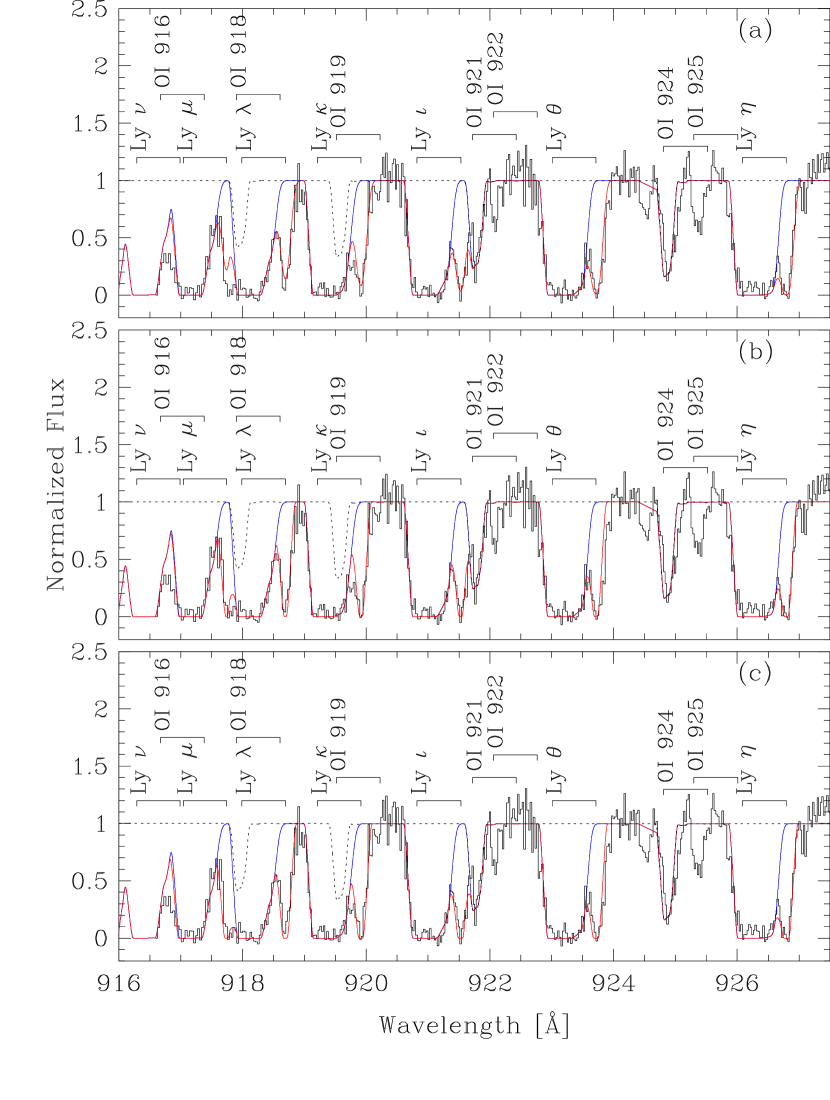
Figure 6: Normalized flux versus wavelength for the high order H I Lyman series and O I transitions detected in the FUSE SiC2A channel in the wavelength range 916–927.5 Å. The flux is plotted as a histogram with 10 km s^-1 bins. The dashed (blue) curve in each panel shows the model of the intermediate velocity and Galactic absorption as described in the text. The dotted curve shows the contribution to this curve from O I absorption as implied by the fit to the 1302.168 Å transition. The thick solid (red) curve in each panel shows the same model with the inclusion of a high velocity component at $v_{\mathrm{LSR}}\approx 184$ km s^-1 under three scenarios: (a) assuming the H I column density derived from direct integration of the Lyman $\lambda$ line, $\log N$(H I)$=16.73$; (b) assuming the model derived from fitting the curve of growth, $\log N$(H I)$=17.82$; and (c) assuming an H I column density at the detection limit of the Wakker et al. (2003) 21 cm emission spectrum, $\log N$(H I)$=18.3$. The parameters of these models are listed in Table 6.

With this fit of the O I profile in hand, we proceeded to model the higher order Lyman series lines (in particular, the Lyman $\eta-\mu$ lines detected in the FUSE SiC2a spectrum). In this H I model, we fixed all the parameters from the fit to the O I profile [component velocity, $b$(O I), $N$(O I)]. We also fixed the H I column densities of the $v_{\mathrm{LSR}}\approx-44,-7,+27$, and +56 km s^-1 components to the values implied by a solar metallicity: $\log N$(H I)$=19.83,19.70,17.29$, and 17.58, respectively. We added the $v_{\mathrm{LSR}}\approx 100$ km s^-1 component back in, fixing the velocity, but allowing the H I column density and $b$-value [as well as the $b$-values of the components not detected by Wakker et al. (2003)] to vary. Instead of allowing the H I column density of the $v_{\mathrm{LSR}}\approx+184$ km s^-1 HVC to freely vary, we considered two extreme cases, the limits implied by the direct integration of the Lyman $\lambda$ profile [$\log N$(H I)$\geq 16.73$], and the non-detection in the Wakker et al. (2003) 21 cm spectrum [$\log N$(H I)$\leq 18.3$]. We fixed the H I column density of the HVC at these two values and allowed the $b$-value to vary. These new models were synthesized assuming Voigt-broadened components and then convolved with a normal distribution having a full-width at half-maximum intensity of 20 km s^-1 to mimic the FUSE instrumental resolution. The least-squares optimized fit parameters are listed in Table 6 (along with the corresponding O I parameters from the preliminary fit). In Figure 6 (panels a and c), we show the best-fit models for the two extreme cases, along with the same model without the contribution of the HVC, for the higher order Lyman series. In addition, we show the contribution of the O I absorption. The differences in the two extreme cases are minor, with the most significant change arising in the Lyman $\mu$ transition. Neither model can be clearly ruled out at the $2\sigma$ level. We therefore consider this full range a 95% confidence interval for the H I column density.

The model used in panel b was derived using our second approach toward constraining the H I column density - a curve of growth fit to the H I equivalent widths reported in Table 2. Assuming that the profiles are formed via a single Voigt-broadened component with a column density $N$ and Doppler width $b$, the equivalent widths $W_{\lambda}$ can be predicted and fit to the observations. In Figure 7, we plot $W_{\lambda}/\lambda$ versus $f\lambda$ for the Lyman series lines detected in the FUSE SiC2 and LiF1 channels using the equivalent widths reported in Table 2. In the figure, we plot two sets of error bars, one for the $1\sigma$ statistical$+$continuum placement error (solid), and one reflecting an additional $10$ km s^-1 uncertainty in the choice of integration range (dashed). The column density and $b$-value that best fit the plotted equivalent widths are $\log N$(H I)$=17.82_{-0.14}^{+0.12}$, $b=14.7\pm 0.4$ km s^-1, and the curve of growth is overplotted in the figure. The central panel of Figure 6 shows the full model using these parameters for the H I HVC absorption. In addition, two other curves of growth using the model parameters of the two extreme cases considered above are also overplotted. From Figure 7, it appears that the two extreme cases listed in Table 6 are unable to reproduce the observed equivalent widths of the stronger Lyman series lines (e.g., Lyman $\beta$, $\gamma$, $\delta$). Visual inspection of the synthetic profiles for lower order H I Lyman series lines revealed that the high velocity side of the absorption profiles are reproduced well. However, it is conceivable that some of the high velocity absorption is missed due to the lower velocity cutoff in the integration (140 km s^-1) and therefore not incorporated into the measurements. We adopt the curve-of-growth results and $1\sigma$ errors in our following estimation of (O/H).

7.2.3 The O/H Abundance

From the preceding analysis, we have constrained the O I and H I column densities to: $\log N$(O I)$=13.82_{-0.03}^{+0.09}$, and $\log N$(H I)$=17.82_{-0.14}^{+0.12}$. Using these adopted values, we estimate that the metallicity of the neutral phase of the high velocity gas is [O/H]$=-0.66_{-0.16}^{+0.39}$, or about $0.14-0.42Z_{\odot}$ ($1\sigma$ confidence). This estimate assumes that the neutral gas arises in a single phase of gas, which is a reasonable approximation considering the shape of the O I $1302.169$ Å line shape. If the $b$-values obtained in the fitting process arise from a contribution of thermal broadening from a Maxwellian distribution and turbulent broadening (which can be characterized by a Gaussian of width $b_{\mathrm{turb}}$), we can constrain the separate contributions of these broadening mechanisms: $b^{2}={{2kT}\over{m}}+b_{\mathrm{turb}}^{2}$, where $k$ is the Boltzmann constant, and $m$ is the mass of the atom. From the inferred $b$-values of O I and H I, we place the following constraints on the two values: $T=11400\pm 800$ K, $b_{\mathrm{turb}}=1.9\pm 0.7$ km s^-1. These quantities should be considered rough gauges of the temperature and turbulence in the neutral gas since the absorption may contain substructure that is blended in velocity.

In addition to the metallicity, we can consider the abundances of other elements relative to oxygen in the neutral phase of the high velocity gas. Of the ions with transitions observed, the following are expected to dominate in a neutral phase: C II, N I, O I, Mg II, Si II, P II, S II, Fe II. (Most of these are singly ionized stages, for which the ionization potential for creation is below 13.6 eV.) If the relative abundances in this neutral phase followed a solar pattern (Table 7) with no ionization corrections the predicted elemental column densities implied by the O I column density [$N$(X)=$N$(O I)$\cdot$(X/O)_⊙] would be $\log N$(C)$=13.75$, $\log N$(N)$=13.09$, $\log N$(Mg)$=\log N$(Si)$=12.70$, $\log N$(P)$=10.73$, $\log N$(S)$=12.43$, and $\log N$(Fe)$=12.61$. Comparison of these scaled column densities with the column densities reported in Table 4 reveals that the column density for every detected singly-ionized species listed above exceeds the expected column density for neutral gas. (The column density upper limits on neutral and other singly-ionized species covered by our dataset are not sufficiently restrictive to place useful constraints on relative abundances.) There are only two possible scenarios that can explain this: (1) the relative elemental abundances deviate from the solar pattern, or (2) ionized gas contributes significantly to the observed column densities. While the former scenario might explain the relative abundance of iron to oxygen with the invocation of different enrichment scenarios, it is unlikely to explain the relative abundances of oxygen, magnesium, and silicon, which are all $\alpha$-process elements. We conclude that there are significant ionization corrections for this low-ionization material which must be considered in order to constrain the relative elemental abundances of the HVC. To first order, we can roughly estimate the magnitude of this ionization correction by considering the Si II column density, since the apparent column density profile of Si II appears to trace that of O I (see Figure 5). Using the predicted and observed column densities for Si II, we estimate that ionized gas contributes $\gtrsim 90$% ($3\sigma$ confidence) of the observed column density. This implies a substantial ionization correction is needed to transform Si II to a total silicon abundance in the cloud. The correction could, in fact, be larger if the HVC contains dust, since the ionization correction only accounts for the gas phase atoms. In the next section, we examine various scenarios to explain the ionization of this gas.

7.3 Ionization

As we have pointed out in the previous sections, in order to infer relative abundances of metals and address, for example, the possible presence of dust, it is imperative to consider the effects of ionization on the observed column density ratios. Understanding the ionization is important as such an analysis yields information on the structure of the gas, the mass contained in the neutral and ionized gas, and constraints on the possible locations of the gas.

In the previous section, we estimated the approximate contribution of the neutral phase (where O I is produced) to the observed column densities of low-ionization species, motivating the need for an additional low-ionization phase. We can apply a similar first order comparison of the amount of high-ionization gas producing the O VI to the neutral gas producing the O I. The relative amounts of gas in each phase can be estimated though the column densities of O VI and O I corrected for their relative ionization fractions ($f$), and abundances [(O/H)]:

$${{N(\mathrm{H})_{\mathrm{HIG}}}\over{N(\mathrm{H})_{\mathrm{NG}}}}={{N(\mathrm{O~{}VI})f_{\mathrm{O~{}VI}}^{-1}\mathrm{(O/H)}_{\mathrm{HIG}}^{-1}}\over{N(\mathrm{O~{}I})f_{\mathrm{O~{}I}}^{-1}\mathrm{(O/H)}_{\mathrm{NG}}^{-1}}},$$ (4)

where the subscripts HIG and NG denote high-ionization gas and neutral gas, respectively. We assume that the oxygen abundances of the two phases are similar [(O/H)_HIG $\approx$ (O/H)_NG] and that all the oxygen in the neutral gas is in the form of O I ($f_{\mathrm{O~{}I}}\approx 1$). The ionization fraction of O VI rarely exceeds 20% (Sembach et al., 2003; Tripp & Savage, 2000), so we can place a lower limit on amount of gas in the high-ionization phase relative to the neutral phase: ${{N(\mathrm{H})_{\mathrm{HIG}}}\over{N(\mathrm{H})_{\mathrm{NG}}}}\gtrsim 0.2^{-1}\times 10^{14.00}/10^{13.82}=7.6$.

For a more detailed understanding of the ionization of the high velocity gas, we consider the kinematics of the HVC to motivate the scenario under which the gas is ionized. The apparent column density profiles shown in Figure 5, which are ordered in ionization potential of the depicted species, provide a starting point. The complex kinematics of the profiles easily rule out absorption originating in a medium having a single density and temperature. It is physically impossible to explain, for example, the drastically different kinematics of O I and O VI in such a phase. However, the velocity alignments of the profiles suggest a common origin. This rules out scenarios such as pure photoionization by the extragalactic background in a low density plasma (e.g., Nicastro et al., 2002). Furthermore, variants of this type of scenario also have difficulty explaining both the ionization of the HVC and the kinematical properties of the high velocity absorption lines.

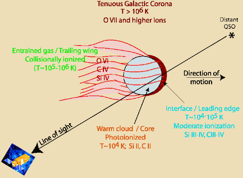
Figure 8: Schematic illustration of the model proposed to explain the high-velocity absorption observed at $v_{\mathrm{LSR}}\approx+184$ km s^-1. A cloud of gas with temperature $\approx 10^{4}$ K is moving through a hotter ($>10^{6}$ K), low-density medium such as the Galactic corona. The interaction between the external medium and the cloud strips material off the cloud. This stripped material becomes entrained in the external medium, adopting its temperature and velocity over time. We draw a possible sight line and label locations for the possible production of low-, moderate-, and high-ionization species corresponding to the velocity regions discussed in §7.3. See Quilis & Moore (2001) and Murray & Lin (2004) for the results of detailed hydrodynamic simulations of this scenario.

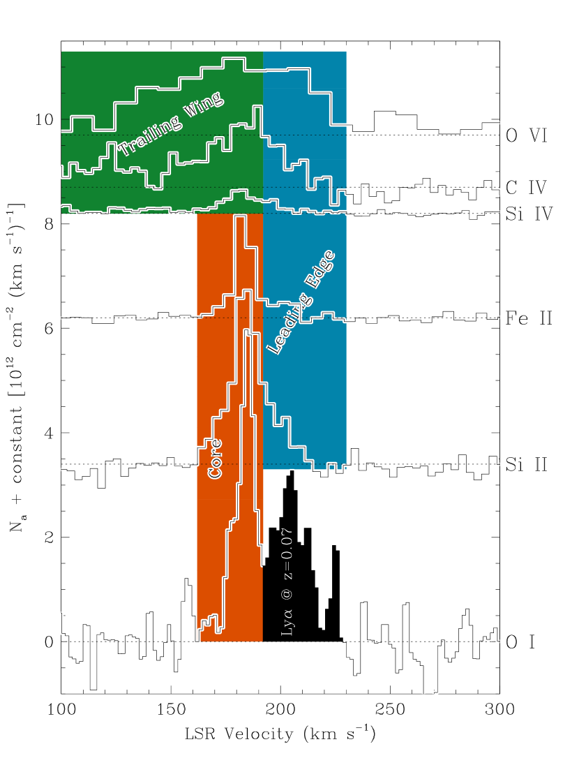
Figure 9: In the above panels, we overlay the apparent column density profiles O I, Si II, Fe II, Si IV, C IV, and O VI. The profiles are offset for clarity, and are shown with a sampling of the two bins per resolution element. We shade and label the three kinematic regions discussed in the text - “Core,” “Leading Edge,” and “Trailing Wing.” The velocities in O I which are blended with a weak Lyman $\alpha$ cloud at $z=0.0719$ is shaded in black. The kinematic distribution of the profiles as a function of ionization is readily apparent.

We propose that the kinematics and ionization of the high velocity gas are qualitatively consistent with a diffuse cloud that is moving away from the Galactic disk and is being stripped by a hot, low-density external medium such as the Galactic halo or corona. A schematic depiction of the cloud structure is shown in Figure 8. The neutral gas resides in the core of the cloud, with some low ionization gas surrounding it. A leading “shock” may exist depending on the density contrast between the cloud and external medium. [It is unlikely to be a classical shock as the velocity of cloud is of the same order as the sound speed of a hot ($>10^{6}$ K), low density ($\lesssim 10^{-4}$ cm^-3) external medium.] As the stripped matter equilibrates with the external medium, it will heat up and slow down. For a fully self-consistent and proper comparison of the observed profiles with such a scenario, one needs a detailed hydrodynamical simulation (e.g., Quilis & Moore, 2001; Murray & Lin, 2004) which is beyond the scope of this paper. Instead, we focus on three key observational features of the absorption that support this scenario - the core ($162\lesssim v_{\mathrm{LSR}}\lesssim 192$ km s^-1), the leading edge ($192\lesssim v_{\mathrm{LSR}}\lesssim 210$ km s^-1) of the low ionization gas (which may produce some moderate ionization gas), and finally, the trailing wing ($125\lesssim v_{\mathrm{LSR}}\lesssim 184$ km s^-1) of the highly-ionized gas. The regions depicted in Figure 8 are further illustrated in Figure 9, where we overlay a subset of the apparent column density profiles shown in Figure 5 and shade the regions to be discussed in the following sections.

7.3.1 The Core

The apparent column density profile of the O I indicates that there is a low-ionization/neutral core of absorbing gas. From the profile shapes of the other species, we can associate the following apparent column densities (and $3\sigma$ limits) in the velocity range $162\leq v_{\mathrm{LSR}}\leq 192$ km s^-1 with this phase of gas: $\log N$(O I)$=13.79\pm 0.03$, $\log N$(C II)$>14.20$, $\log N$(Mg II)$>13.0$, $\log N$(Si II)$=13.76\pm 0.04$, and $\log N$(Fe II)$=13.32\pm 0.07$. As we indicated in §7.2, the Doppler widths of the O I and H I allow us to measure the the temperature of this phase if line widths are due to a combination of thermal and turbulent broadening. The temperature of $T\sim 10^{4}$ K implies that the dominant ionization mechanism in this phase is photoionization, since purely collisional processes would yield high ionization fractions of neutral species whose ionization potentials fall below 1 Rydberg. For example, at a temperature of 11,400 K, the ionization fraction of C I assuming collisional ionization balance is 85% (Dopita & Sutherland, 1996), which would imply a column density of $\log N$(C I)$=13.63$ if the C/O relative abundance is solar.

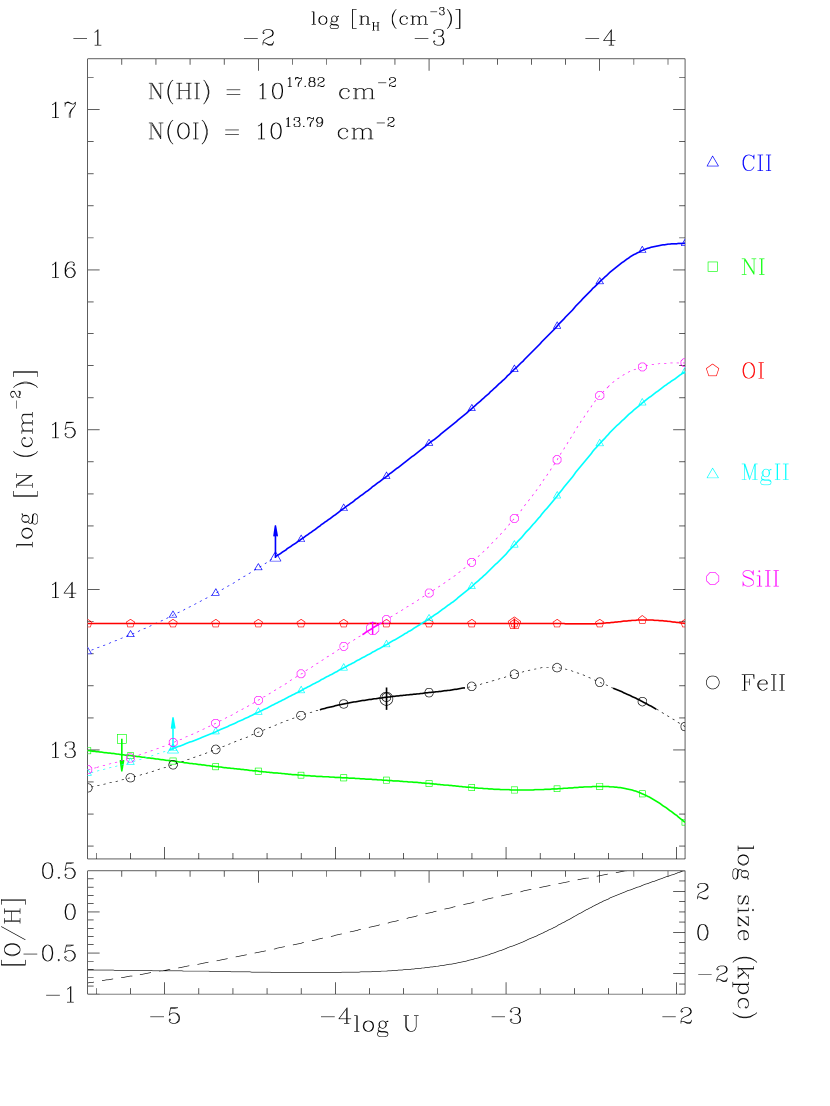
Figure 10: Bottom panel: metallicity (solid line; left axis) and thickness (dashed line; right axis) of a photoionized, plane-parallel slab of gas that reproduces the observed H I and O I column densities of the core region of the +184 km s^-1 HVC. Top panel: predicted column densities of various species assuming a solar relative abundance pattern. The solid portions of the curves correspond to the allowed $1\sigma$ range in column density. The larger symbols with error bars correspond to the observed column densities (or limits) over the integration range $162\leq v_{\mathrm{LSR}}\leq 192$ km s^-1.

In photoionization models, there are two parameters that determine the ionization structure of a gaseous slab - the ionizing spectrum, and the gas density. (To a lesser degree, the metallicity of the gas can also play a role since cooling processes are related to metal content.) We assume here that the dominant source of ionizing photons is the extragalactic background and that the shape of this background is accurately given by the computation of Haardt & Madau (1996) at $z=0$. We normalize this background to $J_{\nu}(\mathrm{1~{}Ryd})=10^{-23}\,\mathrm{erg~{}cm^{-2}~{}s^{-1}~{}Hz^{-1}~{}ster^{-1}}$ (e.g., Scott et al., 2002) and compute a grid of models with varying gas densities using the Cloudy photoionization code (Ferland, 2001). At each grid point, we assume a plane-parallel geometry, and tune the thickness of the ionized slab to reproduce the H I column density (assuming that the bulk of the H I arises in this cloud core). In addition, we tune the metallicity of the gas to reproduce the observed O I column density. (For slabs with $\log n>-3$, the metallicity is determined directly from the observed O I/H I ratio. For lower density slabs, ionization corrections become important.) We summarize the results of these calculations in Figure 10. The thickness of the slab is shown in the bottom panel as a dashed curve with the scale shown on the right axis. The metallicity is shown in the bottom panel as a solid curve with the scale shown on the left axis. The bottom axis of each panel shows the ionization parameter at the surface of slab, defined as the number density of ionizing photons per hydrogen atom: $U=n_{\gamma}/n_{\mathrm{H}}$. On the top axis, we show the gas density.

Assuming the relative metal abundances occur in their solar proportions (Table 7), we show in the top panel of Figure 10 the predicted column density curves C II, N I, O I, Mg II, Si II, and Fe II. We overplot the integrated column densities of those species at the location where they intersect the predicted curve with larger symbols. The solid portions of the model curves indicate the range over which the model column densities satisfy the observed column density constraints ($1\sigma$ range for measured values and lower limits, $3\sigma$ range for upper limits). There are three competing effects that determine the shapes of these curves. First, the ionization fraction of H I decreases with decreasing density, so the required thickness of the slab (and the total amount of gas) increases. Second, for densities lower than $10^{-3}$ cm^-3, the relative ionization correction between O I and H I becomes important, resulting in larger metallicities. Third, the ionization fractions of the species shown (that is, neutral and singly-ionized species) decrease with decreasing density. The first two effects serve to increase the predicted column density of metal species as the gas density decreases, while the third effect tends to decrease the column density of neutral and low-ionization species.

Since the kinematics of Si II are similar to O I, and since both oxygen and silicon are $\alpha$-process elements, it is reasonable to use the comparison of the column densities of those species to constrain the density (and thereby the level of ionization) of the core. If the models are an accurate description of this phase, we constrain the density of the gas to $\log n_{\mathrm{H}}\sim-2.7$ ($U\sim-3.8$), corresponding to a thermal pressure of $p/k\sim 24$ K cm^-3 and an absorber thickness of $\sim 1$ kpc. Under the approximation of a spherical geometry, the gas mass of this phase is $\sim 10^{4.4}$ M_⊙. (This estimate should treated lightly since the geometry of the cloud is uncertain, and a plane-parallel geometry was assumed in the model.) At this density, and within the range of densities allowed by the Si II, all of the other column density constraints shown are satisfied.

If the HVC is close to the Galactic disk, hot O and B stars can provide an additional source of ionizing radiation (e.g., Collins et al., 2004b; Sembach et al., 2003; Bland-Hawthorn & Maloney, 1999, 2001). In this case, both the normalization and shape of the ionizing spectrum will change, favoring softer photons which will ionize neutral species whose ionization potentials lie below 1 Rydberg. In turn, this would require a larger density to yield a similar ionization parameter. Consequently, if the HVC lies closer to the Galactic disk, then the internal thermal pressure of the core is larger than derived above, and the cloud core is also smaller. The addition of a 35,000 K Kurucz model atmosphere with a normalization of $J_{\nu}(\mathrm{1~{}Ryd})=10^{-21}\,\mathrm{erg~{}cm^{-2}~{}s^{-1}~{}Hz^{-1}~{}ster^{-1}}$ (Bland-Hawthorn & Putman, 2001; Weiner, Vogel, & Williams, 2002) to the extragalactic background would require a gas density of $\sim 0.1$ cm^-3 ($U\sim-4$) in order to provide the proper shielding to explain the observed column densities considered here. (Solar relative abundances are still sufficient.) In this case, the thermal pressure in the cloud core is $p/k\sim 10^{3}$ K cm^-3 and the cloud size is $\sim 30$ pc.

7.3.2 The Leading Edge

The apparent column density profiles of the low-, moderate- and high-ionization species show significant amounts of gas at velocities beyond the cloud core out to about $v_{\mathrm{LSR}}\approx+230$ km s^-1. The profiles in the velocity range show a very striking trend between the maximum velocity of detectable column density and the ionization potential of the species. In Figure 9, where we overlay the apparent column density profiles of O I, Si II, Fe II, Si IV, C IV, and O VI, this trend is readily apparent within the region labelled “Leading Edge.” While the high ionization O VI apparent column density profile extends to $v_{\mathrm{LSR}}=230$ km s^-1, lower ionization species clearly cut off at lower velocities, implying a strong ionization velocity-gradient.

In the context of the proposed model of gas stripped from a cloud, it is difficult to place where this higher-velocity edge arises without a detailed understanding of the velocity field. It is attractive to place the gas in front of the cloud, where there is a direct interaction of the cloud with the hot external medium, and perhaps a weak bow shock (e.g., Quilis & Moore, 2001; Murray & Lin, 2004) depending on the relative velocity and density differential of the interacting medium. The existence, relative importance, and detailed velocities of such a shock are dependent on the speed of the cloud through the medium, the density contrast, and the dark matter content of the cloud. If the hot external medium has a density of $\sim 10^{-4}$ cm^-3 and temperature $\sim 10^{6}$ K (e.g., the Galactic corona, Sembach et al., 2003), then the cloud is moving through the external medium at approximately the sound speed (i.e., with a Mach number of order unity) and has a density contrast of about $n_{\mathrm{core}}/n_{\mathrm{external}}\sim 30$, using the line-of-sight velocity and the core density inferred from photoionization by the extragalactic background. If the cloud is travelling through the halo, where the density of the external medium is $\sim 10^{-3}$ cm^-3, then the density contrast is $\sim 100$ (using the inferred density from photoionization by the combination of the extragalactic background and Galactic starlight). This is within the ranges of density contrasts considered in recent models of the density evolution of clouds moving through hot, low density media Murray & Lin (2004).

7.3.3 The Trailing Wing

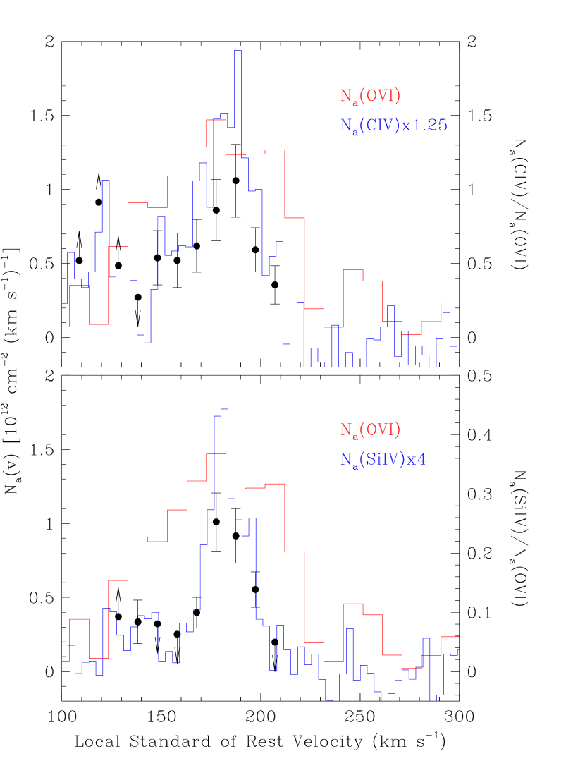
Figure 11: In the above panels, we overlay the apparent column density profiles of O VI (shaded or red histogram) over the apparent column density profiles of C IV$\lambda 1548$ (unshaded or blue histogram, top panel) and Si IV$\lambda 1393$ (unshaded or blue histogram, bottom panel). In each panel, we also plot the apparent column density ratio of the more moderate ionization species relative to O VI (black points, with scales on the right axis).

The trailing tail of gas at velocities smaller than the core absorption, $v_{\mathrm{LSR}}<184$ km s^-1, features statistically significant column densities in high ionization species, O VI, C IV, C III, and Si IV (Figure 9) down to $v_{\mathrm{LSR}}=125$ km s^-1. As with the leading edge, the trailing tail also appears to show a trend of increasing ionization with velocity separation (relative to the core). To further examine this trend, we overlay in Figure 11 the apparent column density profiles of the O VI$\lambda 1031$, C IV$\lambda 1548$ (top panel), and Si IV$\lambda 1393$ (bottom panel). The profiles have been scaled to roughly match the O VI apparent column density at $v_{\mathrm{LSR}}=184$ km s^-1 for ease of comparison, and they shown with a sampling of two bins per resolution element. While the FUSE data of the O VI profile have poorer resolution than the STIS data of the C IV and Si IV profiles, the observed trend of increasing ionization with velocity separation is not a resolution effect, as the wing spans several FUSE resolution elements. In addition to overlaying the apparent column density profiles, we compute the $N_{\mathrm{a}}$(C IV)$/N_{\mathrm{a}}$(O VI) and $N_{\mathrm{a}}$(Si IV)$/N_{\mathrm{a}}$(O VI) ratios as a function of velocity and overplot those as points in the same panels. The points were computed by integrating over the velocity range encompassed by the each bin of the O VI profile (each bin corresponds to half of a FUSE resolution element, or about 10 km s^-1). (We did not use the composite profiles for this exercise.) The points are shown with $1\sigma$ error bars when the integrated apparent column densities are larger than three times their errors, and the absorbed flux is larger than the $1\sigma$ RMS in the continuum. Arrows are drawn on points which represent $3\sigma$ confidence limits. The ionization trend is clear, with both ratios having a peak value at the core of the profile, and decreasing (as the O VI column density becomes larger relative to the other two ion column densities) with decreasing velocity. In the context of the stripped-gas model we have proposed, it is easier to place this lower-velocity gas, since the gas that is stripped should take on the velocity and physical conditions of the hot external medium.

8 Discussion

A high velocity cloud at $v_{\mathrm{LSR}}\approx+184$ km s^-1 in the high Galactic latitude sight-line toward the quasar PG $1116+215$ is detected in absorption over a wide range of ionization species from neutral O I to high-ionization O VI. The kinematic alignment of all detected species implies that these arise from a common structure. Such a structure must contain multiple ionization phases, since it is physically impossible for O I and O VI to arise from a single phase. From the high-quality FUSE and HST/STIS data, we are able to infer a number of properties for this isolated cloud. The detection of O I is fortuitous, since it provides a robust constraint (in tandem with H I information) on the metallicity of neutral gas within the cloud. We estimate a metallicity of [O/H]$=-0.66_{-0.16}^{+0.39}$. The systematic uncertainty is quite large, unfortunately, since the Lyman series lines lie on the flat part of the curve of growth. Nevertheless, comparison of the of the O I and Si II column densities implies that the neutral phase contributes no more than 10% of the observed low-ionization gas. Furthermore, comparison of the O VI to O I implies a highly ionized to neutral gas ratio of at least $\sim$8. In summary, the relative proportions of gas in the neutral, low-ionization, and high-ionization phases are roughly 1:10:8. This implies that substantial ionization corrections are necessary to convert ion column densities to total elemental column densities. We have proposed a possible scenario whereby a dense cloud of gas is streaming through the Galactic corona, and have pointed out various kinematic features - a core of neutral gas, a leading edge of ionized gas, and trailing tail of highly-ionized gas - to lend credence to this scenario. Detailed hydrodynamic modelling to properly and self-consistently account for photoionization and non-equilibrium collisional processes is required to test whether this scenario can account for specific kinematic shapes and column densities of the ions presented.

Ultimately, we would like to constrain the location of the high-ionization high-velocity clouds, the origin of the gas, the ionization mechanism, and mass contained therein. Many models have been proposed, ranging from expanding superbubbles which originate from the Galactic disk, to Local Group gas raining down on the Milky Way, to a local filament of warm-hot intergalactic medium encompassing the Local Group. With the addition of this work to that of Collins, Shull, & Giroux (2004b) and Fox et al. (2005), we have a detailed examination of the high-ionization high velocity clouds toward five sight-lines (PG 1116+215, Markarian 509, PKS 2155–304, HE 0226–4110, and PG 0953+414), which are not readily associated with one of the structures detected in H I 21 cm emission (e.g., the Magellanic Stream, Complex C, etc.). Sembach et al. (2003) and Fox et al. (2005) note that the sight line toward HE 0226–4110 passes $10\fdg 8$ from the $N$(H I 21 cm)$=2.0\times 10^{18}$ cm^-2 contour presented by Morras et al. (2000). Fox et al. (2005) report $\log N$(H I)$\approx 16.3$ for the HVCs detected in the sight line. Thus, it is possible that those HVCs are associated with an extension of the Magellanic Stream. While nine HVCs is probably insufficient to draw gross conclusions about the general population of high-ionization HVCs, it is interesting to compare the conclusions of Collins et al. (2004b), Fox et al. (2005), and this work.

We first note that the HVCs observed toward PG 1116+215 (as well as those observed toward HE 0226–4110 and PG 0953+414) have large positive velocities with respect to the Local Standard of Rest, in contrast to the HVCs toward PKS 2155–304 and Mrk 509, and Complex C which have large negative velocities. Collins et al. (2004a) have examined a simple model of gas falling toward the Galactic center to consider the effects of Galactic rotation on the observed sky distribution of velocities in the Local Standard of Rest. They find that gas falling with a velocity of 50 km s^-1 will appear at high positive velocities ($v_{\mathrm{LSR}}\geq 100$ km s^-1) for sightlines in the range $225^{\circ}\lesssim l\lesssim 320^{\circ}$, $|b|\lesssim 50^{\circ}$. The sight lines toward PG 1116+215, HE 0226-4110, and PG 0953+414 lie at more extreme latitudes, so the observed velocities imply that the clouds are travelling away from the Galactic center. As further noted by Collins et al. (2004a), these velocities could be reproduced through the inclusion of a Galactic fountain, although the low (albeit uncertain) metallicity of the gas makes such an association difficult.

However, we note that all of the properties of the +184 km s^-1 HVC follow naturally if this gas cloud is related to the Magellanic Stream (MS). There is strong evidence that the MS has a tidally-stripped, leading arm (e.g., Putman et al., 1998), and PG 1116+215 is in the general direction of the leading arm. In this case, the positive velocity of the gas, the metallicity, and the indications that the HVC is interacting with the ambient halo all fit together: (1) the leading arm is expected to have positive velocities in this direction, (2) the HVC metallicity is bracketed by the metallicities observed in the ISM of the Magellanic Clouds, [Zn/H]${}_{\mathrm{SMC}}\sim$-0.6 (Welty et al., 1997), [Zn/H]${}_{\mathrm{LMC}}\sim$-0.3 (Welty et al., 1999), and is similar to the metallicity of the MS leading arm (Lu et al., 1998; Sembach et al., 2001a), and (3) it is known from other sight lines that the MS is interacting with the halo/corona of the Milky Way (Sembach et al., 2003). The Magellanic Stream shows complex 21 cm emission at multiple velocities (Wakker, 2001, and references therein), so some of the other absorption components observed toward PG 1116+215 could also be related to the MS (e.g., the +100 km s^-1 HVC). We note that the PG 1116+215 sight line is outside of the region of the leading arm that is easily recognized in 21 cm emission maps, but this could be due to ionization and/or dissipation of the leading arm, which causes the H I column density to drop below the 21 cm detection threshold. It is also possible that the +184 km s^-1 HVC is not strictly “leading arm” material, but rather is gas that was lost by the Magallanic Clouds during a previous orbit. In this case, the passage of time could have reduced $N$(H I), for example, by ionization.

A possible counter-argument to an association with the leading arm of the Magellanic Stream is the relative abundance pattern observed in the low-ionization species. Our photoionization model of the neutral and singly-ionized species in the cloud core shows that the observed column densites are readily explained with solar relative abundances. While the overall metallicity of the cloud is consistent with that of the MS leading arm, there are marked differences in the observed dust content, and depletion patterns. Sembach et al. (2001a) report the detection of H₂ in the MS leading arm in Lyman and Werner absorption against the spectrum of the bright Seyfert 1 galaxy NGC 3783 ($l=287\fdg 5$, $b=23^{\circ}$). No molecular hydrogen is detected in the PG 1116+215 +184 km s^-1 HVC. In the MS leading arm, Si and Fe show signs of appreciable depletion by 0.2 and 0.9 dex, respectively. Such a change to the relative abundances of Si and Fe cannot explain the observed column densities in the PG 1116+215 +184 km s^-1 cloud core, if the photoionization model is accurate. It is important to note, however, that the low-latitude sight line to NGC 3783 passes through a dense region of the leading arm where the contribution of ionized gas to the observed column densities of singly-ionized species is small ($\lesssim 10-15$%). The gas in the high-latitude PG 1116+215 +184 km s^-1 cloud core, on the other hand, is predominantly ionized and more diffuse. Sembach et al. (2001a) estimate a density of $n_{\mathrm{H}}=3.3$ cm^-3 for the H₂ in the low-latitude gas, which is at least 10 times larger than the density in the PG 1116+215 +184 km s^-1 cloud core inferred from our photoionization model. In the PG 1116+215 +184 km s^-1 HVC, we observe $N$(Fe II)$/N$(Si II)$=0.41$, whereas in the MS leading arm toward NGC 3783, Sembach et al. (2001a) observed $N$(Fe II)$/N$(Si II)$=0.18$. This difference is most readily explained by a combination of ionization and differing degrees of heavy metal incorporation into dust grains. With the available data, it is not possible to unambiguously distinguish between these two effects, both of which modify N(Fe II)/N(Si II) in lower density environments where the ionization level is typically higher and the grain destruction is usually more complete than in denser, mainly neutral regions. Thus, it is still possible that the observed differences may be explained by the destruction of dust grains, dissociation of molecules and ionization as the MS leading arm gas continues to interact with the hotter external medium, particularly if the high-velocity gas toward PG 1116+215 (and perhaps PG 0953+414) is remnant stream material from an earlier (older) stream passage.

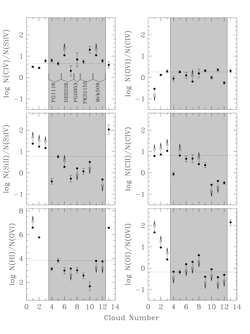
Figure 12: This figure shows various column density ratios for the clouds in the PG $1116+215$ sight line (clouds 1–5), as well as the high velocity clouds toward HE $0226-4110$ (clouds 6–7, Fox et al., 2005), PG $0953+414$ (cloud 8, Fox et al., 2005), PKS $2155-304$ (clouds 9–10, Collins et al., 2004b), Mrk 509 (clouds 11–12, Collins et al., 2004b), and Complex C (cloud 13, Collins et al., 2003; Fox et al., 2004; Sembach et al., 2004a). See Table 9 for further information on the clouds. The shaded region highlights the column density ratios for the highly-ionized HVCs studied in detail thus far. The dashed horizontal line marks the ratio for the $v_{\mathrm{LSR}}=+184$ km s^-1 HVC in the PG $1116+215$ sight line (cloud 5).

We can compare the gross characteristics of the highly-ionized HVCs by considering various column density ratios. In Table 8, we reproduce the column density ratios reported for the high velocity clouds toward PKS 2155–304, and Mrk 509 (Collins et al., 2004b, see their Table 5 for notes), and for Complex C as observed along the PG 1259+593 sight line (Collins, Shull, & Giroux, 2003; Fox et al., 2004; Sembach et al., 2004a). We add three additional high velocity clouds from Fox et al. (2005), and two high velocity clouds from this work as well as the three Galactic ISM/IVC components observed along the PG 1116+215 sight line. For comparison, we plot these ion ratios in Figure 12 (see Table 9 for the ordering of clouds in the figure). The column density ratios for the HVCs toward PG 1116+215, HE 0226–4110, PG 0953+414, PKS 2155–304 and Mrk 509 tend to favor higher ionization gas, as evidenced by the O I/O VI constraints, in stark contrast to the low/intermediate-velocity clouds toward PG 1116+215 and Complex C. There is a clear distinction between Complex C (and the low/intermediate velocity gas) and the high-ionization HVCs, with the former being dominated by H I and the latter being dominated by H II. This separation is also apparent in the Si II/Si IV ratio.

A possible argument against a Galactic origin for the highly-ionized HVCs would be a comparison of the $N$(C IV)$/N$(Si IV) column density ratio. As reported by Sembach et al. (1997) in a study of Radio Loops I and IV, this ratio remains fairly constant close to and within the Galactic disk: $\log N$(C IV)$/N$(Si IV)$=0.58_{-0.30}^{+0.18}$. Of the nine high-ionization HVCs, only three are actually inconsistent with this range, the $v_{\mathrm{LSR}}\approx+145$ km s^-1 HVC toward HE 0226–4110, the $v_{\mathrm{LSR}}\approx-270$ km s^-1 HVC toward PKS 2155–304, and the $v_{\mathrm{LSR}}\approx-240$ km s^-1 HVC toward Mrk 509. Collins et al. (2004b) note that the $N$(C IV)$/N$(Si IV) ratio for the HVCs toward PKS 2155–304 and Mrk 509 are significantly higher than the ratio for gas within the Galactic disk or low halo, and argue against a location close to or within the disk. The same ratio for the $v_{\mathrm{LSR}}\approx+184$ high velocity cloud is not only consistent with the ratio reported by Sembach et al. (1997), but is also consistent with the ratio reported by Collins, Shull, & Giroux (2003) for Complex C. However, as summarized by Fox et al. (2004), there are several collisional processes that can potentially explain the observed range of C IV/Si IV. Thus, for the majority of the highly-ionized HVCs that have been observed to date, we cannot rule out an origin near (or within) the Galactic disk based on the $N$(C IV)$/N$(Si IV) column density ratio.

Further comparison of the observed O VI/C IV column density ratios to the predicted ranges for the collisional processes considered by Fox et al. (2004) reveals that conductive interfaces and shock ionization can account for observed ratios for both the highly-ionized HVCs (with one exception - $v_{\mathrm{LSR}}\approx-300$ km s^-1 toward Mrk 509) and Complex C (see Table 5 for a summary of the model parameters and ranges considered). Thus, while the origins of HVCs may be varied (as indicated by the differences in abundance patterns of the neutral/low-ionization species), there may be a common mechanism (or mechanisms) for the production of the high-ionization species. In particular, the interaction of the HVCs with a hot medium such as the Galactic halo or corona can account for the ionization patterns observed. The ratios of high ionization species for the highly-ionized HVCs are inconsistent with radiative cooling processes (see Table 5), which is presumably the dominant process in the collapse of a large scale filament. This lends additional credence to the idea that at least some of the high-ionization HVCs reside either in the outer Galactic halo or the more extended, lower-density corona (as opposed to the Local Group or the WHIM). It is unlikely that the gas lies within a few kiloparsecs of the Galactic disk, since the ion column density ratios favor higher ionization species as compared to the low/intermediate-velocity gas in this same sight line. For this reason, it is also more likely that the highly ionized HVCs result from infalling material or tidally stripped material than from gas ejected from the Galactic disk by supernova explosions.

9 Summary

The primary results of this study are as follows:

• We have obtained high resolution FUSE and HST/STIS echelle observations of the quasar PG $1116+215$. The semi-continuous coverage of the ultraviolet spectrum over the wavelength range 916–2800 Å provides detections of Galactic and high velocity absorption over a wide range of ionization species: H I, C II-IV, N I-II, O I, O VI, Mg II, Si II-IV, P II, S II, and Fe II.

• The high spectral resolution of these data (6.5-20 km s^-1) yields kinematic information for the Galactic, intermediate, and high velocity absorption over the velocity range $-100<v_{\mathrm{LSR}}<+300$ km s^-1, which provides an important a priori starting point in the analysis of the absorption profiles. We have constructed composite apparent column density profiles for species where multiple unblended transitions are available within a given instrumental setup. These are valid, instrumentally-smeared profiles with a large dynamic range in column density. In particular, we are able to fully recover the apparent column density profiles of Si II and Fe II at 6.5 km s^-1 and 10 km s^-1 velocity resolution, respectively.

• In the low and intermediate ionization species, we detect two high velocity clouds at $v_{\mathrm{LSR}}\approx 100$ km s^-1 and $v_{\mathrm{LSR}}\approx 184$ km s^-1. The $v_{\mathrm{LSR}}\approx 100$ km s^-1 component is detected as an absorption feature in the C II$\lambda 1334.532$, Si II$\lambda 1260.422$ and Si III$\lambda 1206.500$ transitions. Blended and/or saturated absorption at this velocity exists in the other higher ionization species (i.e., C III, C IV, O VI, Si IV), while no detectable absorption exists in other low ionization or neutral species. The high velocity cloud at $v_{\mathrm{LSR}}\approx 184$ km s^-1 is detected over a large range of ionization species, from neutral O I to highly ionized O VI, with striking kinematics differences.

• The apparent column density profile of O I in the $+184$ km s^-1 HVC has a narrow discrete component that is apparent in other low ionization species. In the singly-ionized species, there also appears to be a shelf of column at slightly higher (i.e., more positive) velocities than the neutral core traced by O I. In the high ionization species (e.g., C IV, O VI), the profiles are broad, and asymmetric, with a tail of absorption extending toward lower velocities.

• Since there is essentially no relative ionization correction between O I and H I, we have attempted to measure the metallicity of the neutral HVC gas using column density ratios of these two species. The higher order H I Lyman series lines suffer from saturation, and therefore do not tightly constrain the H I column density. The best fit curve of growth and profile fit analysis yields an optimal metallicity of [O/H]$=-0.66_{-0.16}^{+0.39}$ (1$\sigma$).

• The Si II/O I ratio provides a measure of the contribution of the neutral gas to the observed column density of low-ionization species. For solar relative abundances of Si and O, we estimate that at most 10% of the Si II column density can be attributed to the neutral gas that produces the O I.

• A simple model of gas with density $10^{-2.7}$ cm^-3, a thickness of $\sim 1$ kpc, and solar relative metal abundances for O, Si, and Fe photoionized by the Haardt-Madau extragalactic spectrum is able to explain the observed column densities (or limits) of the neutral and low-ionization species in the velocity range $v_{\mathrm{LSR}}=$162–192 km s^-1 (i.e., in the cloud core). The addition of ionizing photons from the Galactic disk increases the density and thermal pressure estimates by about a factor of 50, and decreases the absorber thickness by about a factor of 30.

• We have examined the relative contributions of neutral and highly-ionized gas in the high velocity cloud by considering the ratio O VI with respect to O I. In the total velocity range 140–230 km s^-1, the integrated column densities indicate that there is at least $\sim$8 times more highly ionized gas than neutral gas, assuming that highly-ionized gas has a similar metallicity to the neutral gas.

• The qualitative features of the apparent column densities as function of both velocity and ionization suggest an absorbing structure in which a moderately dense cloud of gas is heading away from the Galactic center (or in orbit) and passing through a hot tenuous medium (e.g., the Galactic halo or corona), which is stripping gas off the cloud. The denser core of the cloud gives rise to the neutral species and some low-ionization species. The front of the cloud faces away from the observer at higher velocities and is the prime site where gas is stripped. This front edge produces the more moderate ionization species (e.g., Si III, C III), as well as some high ionization species (Si IV, C IV, O VI). The stripped gas interacts with the hot external medium, takes on the velocity and ionization of that medium, and gives rise to a high-ionization (e.g., O VI) “wake” trailing the cloud at lower velocities.

• In considering this model, it is important to distinguish whether the cloud is travelling through the Galactic halo or the more extended and diffuse Galactic corona, since the ability of the ambient medium to strip gas from the cloud depends on the relative density. If the cloud is travelling through the Galactic corona, its velocity is roughly the sound speed, and the density contrast between the neutral core and the external medium is roughly 30:1. If the cloud is travelling through the Galactic halo, the contrast is of order 100:1.

• To further examine the feasibility of the non-equilibrium scenarios in explaining the absorbing gas, we suggest that future numerical simulations of the evolution of clouds moving through a tenuous medium be accompanied by an exploration of the direct observables (e.g., column densities, line widths, line asymmetries) as a function of ionization stage. This can lead to the formulation of key diagnostics (e.g., column density ratios and line profile shape differences) that can be used to understand the relative importance of different hydrodynamical processes in producing the high velocity gas.

• The ionization structure, kinematical complexity, and column density ratios of the ionic species observed in this high velocity cloud rule out the photoionization models suggested by Nicastro et al. (2002) as an explanation for O VI HVCs in the Local Group (e.g., Nicastro et al., 2002). Rather, this HVC is part of a dynamical system that likely involves complex interactions with the outer regions of the Galaxy, as has been suggested by other authors (e.g., Sembach et al., 2003; Tripp et al., 2003; Fox et al., 2004).

• We suggest that the leading arm of the Magellanic Stream may be the origin of this gas based on the location of the high velocity gas on the sky, and its high positive velocity. The ionization level and the metallicity of the high velocity gas core, and the kinematics of the higher ionization gas, are also consistent with such an origin. Alternatively, the gas could arise from Stream gas from a prior orbit or from a tidally disrupted dwarf galaxy unrelated to the Magellanic Clouds. Further studies of the metallicity and ionization of the positive high velocity gas along other sight lines in this region of the sky could help to clarify the origin(s) of the gas.

Appendix A Description of Individual Ions

• In the STIS/E140M spectrum, we cover four strong transitions of the C I ion at 1277.245 Å, 1328.833 Å, 1560.309 Å, and 1656.928 Å. The relative values of $f\lambda$ of these lines (with the exception of 1560.309 Å) have been investigated by Jenkins & Tripp (2001), who find systematically higher values of $f\lambda$ for lines with smaller published $f\lambda$. We adopt their values over those listed in Morton (2003) for the 1277.245 Å, 1328.833 Å, and 1656.928 Å lines. [The line at 1560.309 Å was not considered in the Jenkins & Tripp (2001) analysis, and we adopt the Morton (2003) data.] An additional transition at 945.191 Å is also covered by the FUSE data. There is a weak unidentified absorption feature $\sim$160 km s^-1 blueward of the 1277.245 Å line, but it does not affect any of our measurements. In addition, there is a weak, broad Lyman $\alpha$ line at $z=0.0928$, which is blended with the 1328.833 Å line, but it was easily removed in the continuum-fitting process. In the top panel of Figure 3a, we overlay the apparent column density profiles of these transitions. Absorption by this ion is only visible in the $v_{\mathrm{LSR}}\approx-44$ km s^-1 intermediate velocity component, where the core apparent optical depth in all transitions is less than unity. The agreement between ACD profiles is reasonable, given the weakness of the lines and the noisiness of the data. The integrated column density of the $v_{\mathrm{LSR}}\approx-44$ km s^-1 absorption is greatly affected by the choice of integration range for this same reason (weak lines and noisy data), so we restrict the integration range of this component to $-60\leq v_{\mathrm{LSR}}\leq-35$ km s^-1. The 1656.928 Å and 1277.245 Å lines yield identical integrated column densities, while the 1560.309 Å and 1328.833 Å lines yield slightly smaller and larger integrated column densities, respectively. We use the three lines with self-consistent line-strengths (1277.245 Å, 1328.833 Å, and 1656.928 Å) to compute our adopted column densities (and limits) for all integration ranges.

• There are two transitions of the C II ion at 1036.337 Å and 1334.532 Å which are covered by our data. Both are detected, the 1036.337 Å line in the FUSE spectra, and the 1334.532 Å line in the STIS-E140M and both suffer from unresolved saturated structure and blends with the associated excited state lines. We use only the 1334.532 Å line for our measurements, and we can derive only lower limits on $N$(C II) in most of the components.

• The only transition of C III covered is the strong 977.020 Å line in the FUSE spectrum. The line saturates at an apparent column density per velocity interval of $5.1\times 10^{11}$ cm^-2 (km s^-1)^-1, and is effectively black (i.e., with an absorbed flux less than the $1\sigma$ above the zero flux level) at an apparent column density per velocity interval of $1.2\times 10^{12}$ cm^-2 (km s^-1)^-1. In all of the integration ranges, the observed flux is less that $1\sigma$ above the zero flux level, and we adopt lower limits on integrated column densities.

• The resonant doublet at $\lambda\lambda$1548.204, 1550.781 is detected in the STIS E140M spectrum (see Figure 1). The 1548.204 Å falls at the edges of two adjacent echelle orders and the data are interlaced to produce the profile shown in Figure 2a and for the subsequent analysis. There is agreement in the integrated apparent column densities between the two transitions over the velocity range encompassing the low- and intermediate velocity gas, $-100\leq v_{\mathrm{LSR}}\leq+85$ km s^-1. Integration over the velocity ranges associated with the two high velocity clouds yield slightly discrepant apparent column densities, although they are consistent within the uncertainties. For the $v_{\mathrm{LSR}}\approx+100$ km s^-1 component, the integrated apparent column densities indicate possible unresolved saturated structure, but this is unlikely to be the case as the apparent optical depths are low. We use both transitions in computing the composite, but use only the 1548.204 Å transition for our adopted column densities in all velocity intervals.

• There are several strong triplets of the N I ion, with the strongest and best separated at $\lambda\lambda$1199.550, 1200.223, 1200.710. The two H I components detected in the Wakker et al. (2003) 21 cm emission profile are detected in this ion, although they are heavily saturated and blended together. Our “standard” treatment for recovering the composite apparent column density profile (described above) using all three transitions is able to recover a clean profile with unresolved saturated structure over those two components and provide clear non-detections in the other three components. For our adopted N I column densities, we use the 1200.710 Å transition for the low-velocity clouds and the $v_{\mathrm{LSR}}\approx+100$ km s^-1 HVC since it is unaffected by blending and is the weakest of the three transitions (thus providing the best lower limits in the regions of unresolved saturation). For the $v_{\mathrm{LSR}}\approx+184$ km s^-1 HVC, we use the 1200.223 Å line to derive the best upper limit, since it is unaffected by blends over the integration range and is stronger than the 1200.710 Å transition.

• Only the 1083.994 Å line is covered by our dataset. It is detected in the SiC1 channel of the FUSE spectrum. The line is clearly saturated over the integration ranges of the $v_{\mathrm{LSR}}\approx-44$ km s^-1 and $v_{\mathrm{LSR}}\approx-7$ km s^-1 components and may contain some unresolved saturated structure in the $v_{\mathrm{LSR}}\approx+184$ km s^-1 HVC component and we adopt lower limits for the column density for these components. The absorption is not saturated over the integration of the $v_{\mathrm{LSR}}\approx+56$ km s^-1 component and we quote a value over the integration range +37 km s^-1 to +85 km s^-1. It is not detected at $v_{\mathrm{LSR}}\approx+100$ km s^-1 and we adopt an upper limit on the column density.

• The strong doublet of the high-ionization N V ion at $\lambda\lambda$1238.821,1242.804 is covered in the STIS E140M data and is not detected in any component. The nominal location of the 1238.821 Å line falls on two orders of the echelle, like the C IV$\lambda 1548.204$ line. We use the 1238.821 Å transition to compute the best upper limits on the N V column density for all integration ranges.

• There are several O I lines in the FUSE band which suffer from blends with transitions from other ions (e.g., the H I Lyman series). In the STIS E140M band, we detect the 1302.169 Å line. The low- and intermediate velocity gas in this line suffers from unresolved saturation. The line also falls on two orders of the echelle. We use the 1302.169 Å profile for all integrated column densities, reporting lower limits for the low-velocity components, an upper limit for the +100 km s^-1 HVC and a measurement for the +184 km s^-1 HVC. See §7.2.1 for further examination of possible saturation effects in the O I column density for this HVC.

• The strong doublet at 1031.926 Å, and 1037.617 Å is clearly detected in the FUSE band, and has been presented by Wakker et al. (2003). The 1031.926 Å line is free of blends, while the 1037.617 Å line is blended with H₂ from the $-44$ km s^-1 intermediate-velocity gas. Thus, we only use the 1031.926 Å line for our measurements, and do not attempt to combine the two lines to form a composite ACD profile. Since O VI is not detected in the -44 km s^-1 component, we report an upper limit on the column density.

• The strongest line from Mg I at 2852.963 Å ($\log f\lambda=3.718$) is not covered by our dataset; our STIS E230M spectrum cuts off at 2819.13 Å. However, the weaker lines at 2026.477 Å and 1707.061 Å are covered. These are not detected, and we use the stronger 2026.477 Å line to determine the limiting column densities for all components. The 2026.477 Å line falls on two adjacent orders of the STIS E230M echelle spectrum.

• The strong doublet at 2796.354 Å, and 2803.532 Å is detected in the STIS E230M spectrum. The velocity range $-100\leq v_{\mathrm{LSR}}\leq+40$ suffers from blended saturated structure (the velocities covering the $v_{\mathrm{LSR}}\approx-44$ km s^-1 and $v_{\mathrm{LSR}}\approx-7$ km s^-1 components), and the component at $v_{\mathrm{LSR}}\approx+56$ km s^-1 is resolved, but saturated. For these components we quote lower limits on the integrated apparent column density using the 2803.532 Å line. The high velocity gas at $v_{\mathrm{LSR}}\approx+100$ km s^-1 is not detected, while the high velocity gas at $v_{\mathrm{LSR}}\approx+184$ km s^-1 is marginally saturated. We use the 2796.354 Å transition to compute the best upper limit on the column density for the +100 km s^-1 component, and combine the measurements from both transitions for the $+184$ km s^-1 component.

• There are five transitions covered by the STIS E140M spectrum, which range in line strength $2.051\leq\log f\lambda\leq 3.172$ at 1190.416 Å, 1193.416 Å, 1260.422 Å, 1304.370 Å, and 1526.707 Å. The transitions suffer from blended saturated structure in the velocity ranges which include the $v_{\mathrm{LSR}}\approx-44$ km s^-1 and $v_{\mathrm{LSR}}\approx-7$ km s^-1 components. For these two components, we quote limiting column densities from the integration of the 1304.370 Å line, which is detected in adjacent echelle orders. Likewise, we also use this line to quote a measurement of the $v_{\mathrm{LSR}}\approx+184$ km s^-1 high velocity component, since it is the least affected by unresolved saturated structure. The high velocity cloud at $v_{\mathrm{LSR}}\approx+100$ km s^-1 is only detected in the 1260.422 Å transition and we adopt the integrated column density from this line.

• The only transition of Si III covered by our dataset is at 1206.500 Å. The components at $v_{\mathrm{LSR}}\approx-44$ km s^-1, $-7$ km s^-1, and +56 km s^-1are strongly saturated and blend together. The component at $v_{\mathrm{LSR}}\approx+100$ km s^-1 is optically thick in this transition, as is the component at $v_{\mathrm{LSR}}\approx+184$ km s^-1. We treat the integrated column densities in all components as lower limits.

• The strong doublet at 1393.760 Å, and 1402.773 Å is covered and detected in the STIS E140M spectrum. The 1402.773 Å line falls in two adjacent echelle orders in the velocity region $v_{\mathrm{LSR}}\leq 20$ km s^-1. The 1402.773 Å profile shows some minor inconsistencies with the 1393.760 Å profile. In particular, there is an excess of absorption at $v_{\mathrm{LSR}}\approx 10$ km s^-1. The feature extends over a few pixels and appears to be real as it exists independently in the two echelle orders. It is possible that an unidentified absorption line (e.g., a weak, narrow Lyman $\alpha$ line) contaminates the 1402.773 Å line. For this reason, we use only the 1393.760 Å in our computation of the column density of the -7 km s^-1 component. For other components, we combine the measurements from both transitions.

• The strongest transition of P II which is covered by our dataset is the 963.800 Å line ($\log f\lambda=3.148$). This line is clearly detected in the FUSE band, but is blended with the N I$\lambda\lambda$ 963.990, 963.626, 963.041 triplet and is not useful for our purposes. The strongest transition that is free of blends is the 1152.818 Å line which is covered by both FUSE, and STIS data. The line is detected in the FUSE spectrum, but not in the STIS spectrum due to poor signal-to-noise in that region of our STIS spectrum. The next strongest lines available in the higher resolution STIS spectra are at 1301.874 Å and 1532.533 Å (E140M). The low- and intermediate-velocity components at $v_{\mathrm{LSR}}\approx-44$ km s^-1 and $-7$ km s^-1 are detected in the 1152.818 Å line. No other components are detected. No absorption is detected in the 1532.533 Å line, and the absorption in the expected region of the 1301.874 Å line is dominated by the Galactic O I 1302.619 Å absorption. (Given the strength of the P II 1152.818 Å line, there is no reason expect blending issues with the Galactic O I measurements.) We use the 1152.818 Å line for the column density determinations in all components (measurements for the -44 km s^-1 and -7 km s^-1 components, upper limits for the other components).

• The strongest lines from S I which are covered by our spectra are at 1295.653 Å, and 1425.030 Å. Both of these are covered in E140M spectrum but are not detected. We use the stronger 1425.030 Å line to obtain upper limits on the integrated column densities.

• The only transitions of S II at wavelengths redward of the Lyman limit are covered and detected in the E140M spectrum. The S II $\lambda\lambda$1250.578, 1253.805, 1259.518 lines all show a resolved two component structure at velocities $v_{\mathrm{LSR}}\approx-44$ km s^-1 and $v_{\mathrm{LSR}}\approx-7$ km s^-1. No other velocity components are detected. The 1259.518 Å line has an odd kinematic structure over the velocities spanned by these two components which is not consistent with the other two lines. The structure is apparent in only one order, but we find nothing to suggest that it should not be trusted (e.g., there is nothing odd in the error spectrum). The two detected components contain unresolved saturated structure in this line, so we do not use this transition in our adopted column density measurements. In addition, the integration range for the $v_{\mathrm{LSR}}\approx-44$ km s^-1 component in the 1250.578 Å line is contaminated by Lyman $\alpha$ at $z=0.02845$. Comparison of the apparent column density profiles of the 1250.578 Å and 1253.805 Å lines indicates possible unresolved saturated structure in the 1253.805 Å line. So we quote the integrated column density of the 1253.805 Å line as a lower limit. For the -7 km s^-1 component, we combine the integrated apparent column densities of the 1250.578 Å and 1253.805 Å lines. The integration range for the undetected high velocity cloud at $v_{\mathrm{LSR}}\approx+184$ in the 1253.805 Å line is contaminated by another Lyman $\alpha$ line at $z=0.03223$. Only the 1250.578 Å line is used for the adopted column density upper limit for this component and the +100 km s^-1 and +56 km s^-1 components.

• A suite of Fe II transitions is covered in our STIS E230M dataset. In particular, we detect all transitions in the wavelength range 2249.8–2600.2 Å with line strengths exceeding $\log f\lambda\geq 0.6$. We also detect the transition at 1608.451 Å in the E140M spectrum. The transitions with line strengths exceeding $\log f\lambda\geq 1.87$ suffer from unresolved saturated structure in the velocity range $-100\leq v_{\mathrm{LSR}}\leq+20$ km s^-1. We combine the integrations over the 2260.781 Å and 2249.877 Å lines to determine composite column densities for the $v_{\mathrm{LSR}}\approx-44$ km s^-1 and $v_{\mathrm{LSR}}\approx-7$ km s^-1 components. The component at $v_{\mathrm{LSR}}\approx+56$ km s^-1 is detected in transitions with $\log f\lambda\geq 1.87$. We combine all transitions to compute a composite integrated column density for this component. The high velocity component at $v_{\mathrm{LSR}}\approx+100$ km s^-1 is not detected in any transition (up to $\log f\lambda=2.882$), and we use the 2382.765 Å line to compute an upper limit on the integrated column density. For the high velocity cloud at $v_{\mathrm{LSR}}\approx+184$ km s^-1, there are inconsistencies in the apparent column density profiles to note which affect the computation of a composite column density. The profiles from the 2382.765 Å and 2600.173 Å lines may be affected by unresolved saturated structure, although they yield identical integrated column densities. The 2344.214 Å and 2374.461 Å lines yield systematically (and significantly) smaller and larger integrated column densities, respectively, than the 2382.765 Å and 2600.173 Å lines. If the 2382.765 Å and 2600.173 Å lines are included in the computation of a variance-weighted column density, then they dominate the computation, $\log N_{\mathrm{a}}$(Fe II)$=13.41\pm 0.03$. However, if only the 1608.451 Å and 2586.650 Å lines are used, then we find a slightly larger, though more uncertain, value $\log N_{\mathrm{a}}$(Fe II)$=13.46\pm 0.09$. We adopt this latter value for the integrated column density.

Figure 1: Portions of the spectra from the three observations used in this paper - FUSE (top panel), HST/STIS-E140M (middle panel), HST/STIS-E230M (bottom panel). The plotted regions are centered around key transitions from each observation, and the wavelength scale shown spans about 3300 km s^-1 in all three panels. In each panel, the Galactic ISM profiles are labelled with the absorbing species, and the corresponding +184 km s^-1 HVC absorption are indicated by the offset tick marks.

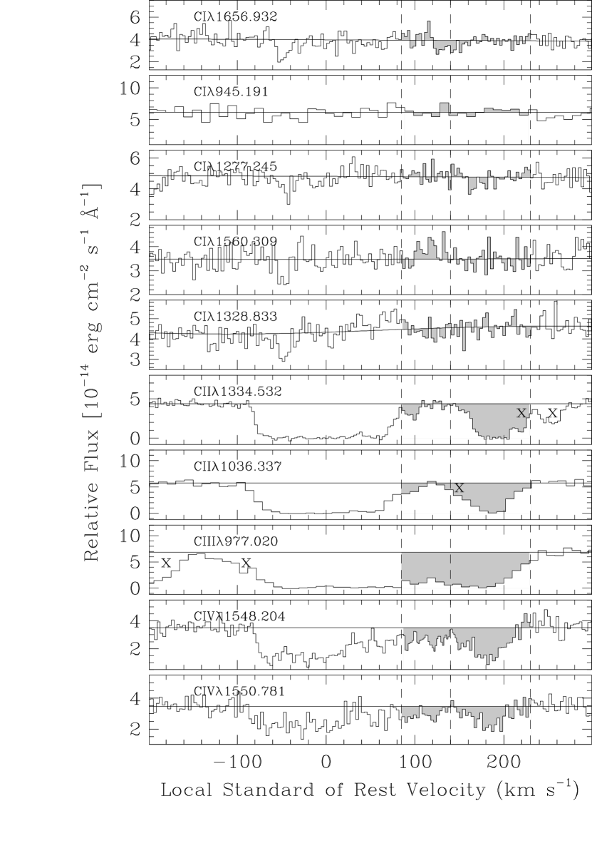
Figure 2a: Flux profiles of selected transitions of carbon ions versus Local Standard of Rest velocity. The profiles are ordered, top to bottom, by increasing ionization stage and decreasing transition strength (within each stage). The velocity range 100–230 km s^-1, over which high velocity absorption is expected (though not necessarily detected), is shaded. The dashed vertical lines at $v_{\mathrm{LSR}}=85$, 140, and 230 km s^-1 mark the integration limits for the HVCs. Regions affected by blends with other absorption features are marked with an ’x’. Note that the scale for the flux axis changes from panel to panel. (See the notes in the appendix and Sembach et al. (2003) for identifications of the blends.) Transitions below 1184 Å are detected in the FUSE spectrum; transitions in the range 1184–1720 Å are detected in the STIS E140M spectrum; transitions above 2000 Å are detected in the STIS E230M spectrum.

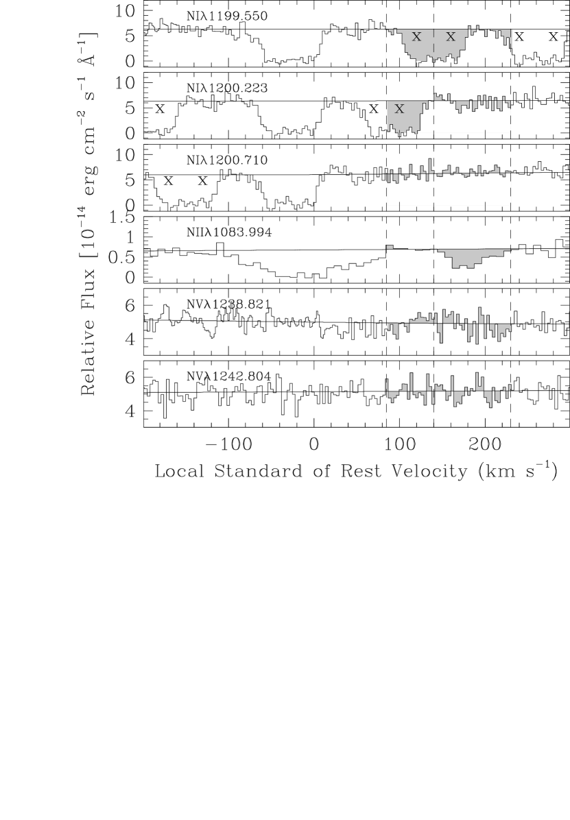
Figure 2b: Same as Figure 2a, but for the ions of nitrogen.

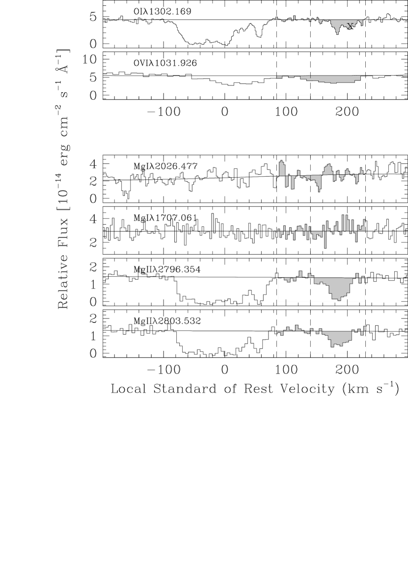
Figure 2c: Same as Figure 2a, but for the ions of oxygen and magnesium.

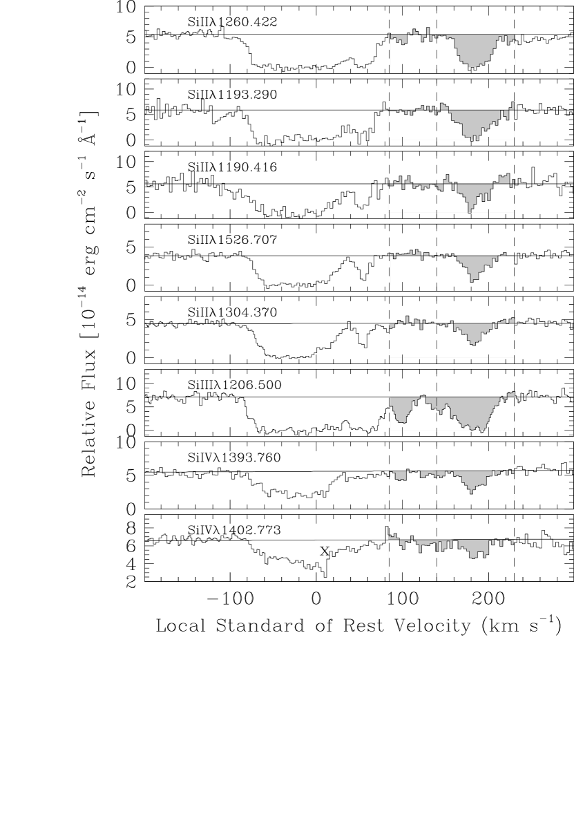
Figure 2d: Same as Figure 2a, but for the ions of silicon.

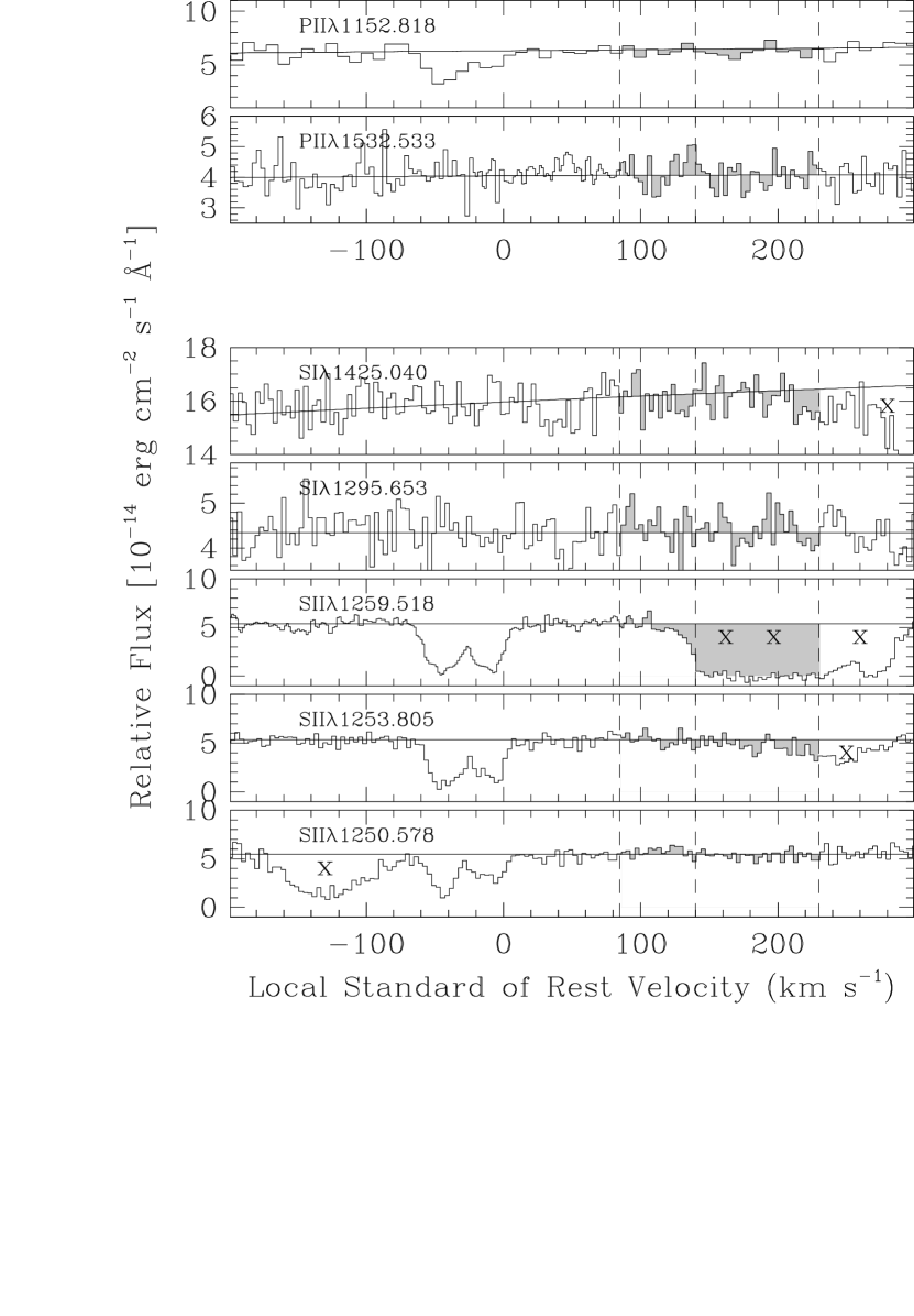
Figure 2e: Same as Figure 2a, but for the ions of phosphorus and sulfur.

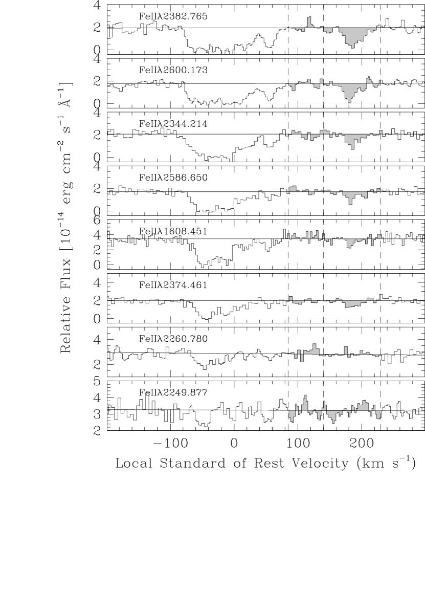
Figure 2f: Same as Figure 2a, but for the ions of iron.

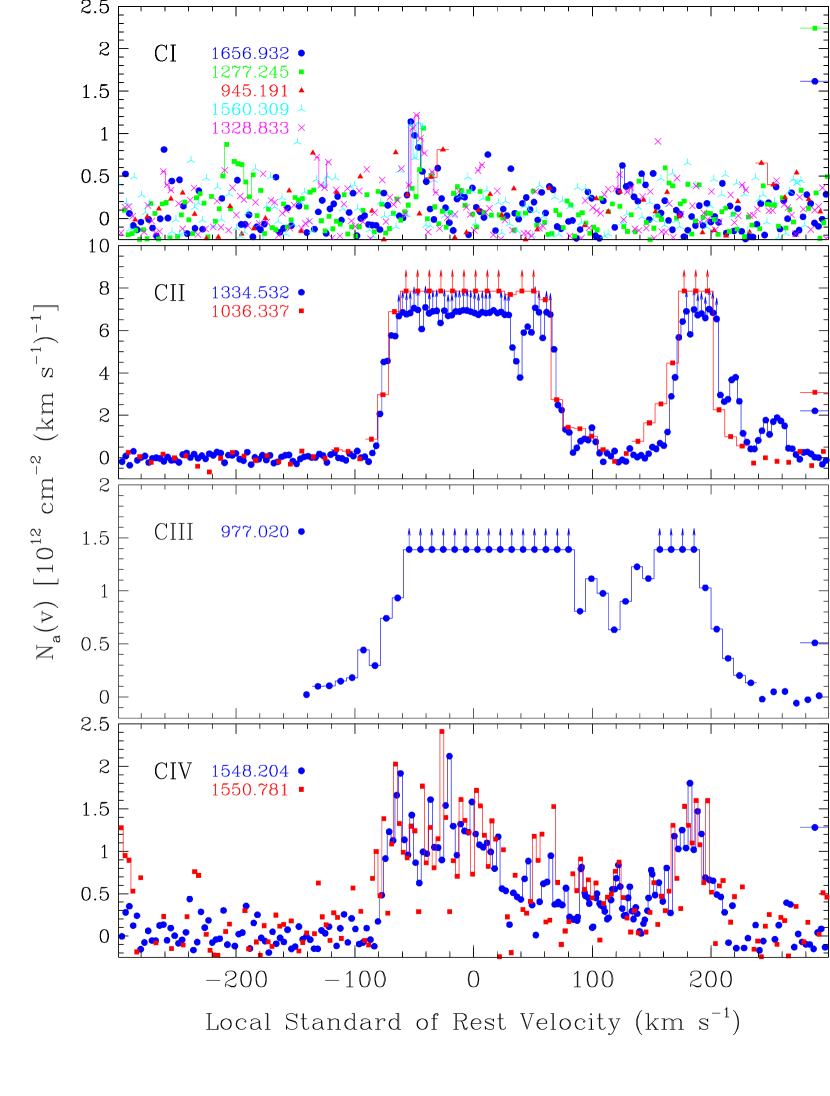
Figure 3a: In the above panels, we show apparent column density profiles versus Local Standard of Rest velocity for a sample of transitions detected in Galactic absorption. Each panel depicts the apparent column density profiles for a given species, with the profile transitions color-coded and over-plotted. A histogram line connects bins where absorption is detected, and arrows indicate bins where the absorbed flux is consistent with zero. A horizontal bar is shown on the right side of the panels at the value of $N_{\mathrm{a}}(v)$ for which the transition reaches an apparent optical depth of unity. For clarity, pixels which are blended with other transitions are not shown (e.g., each member of the N I triplet was cleaned to avoid blends with the other two members).

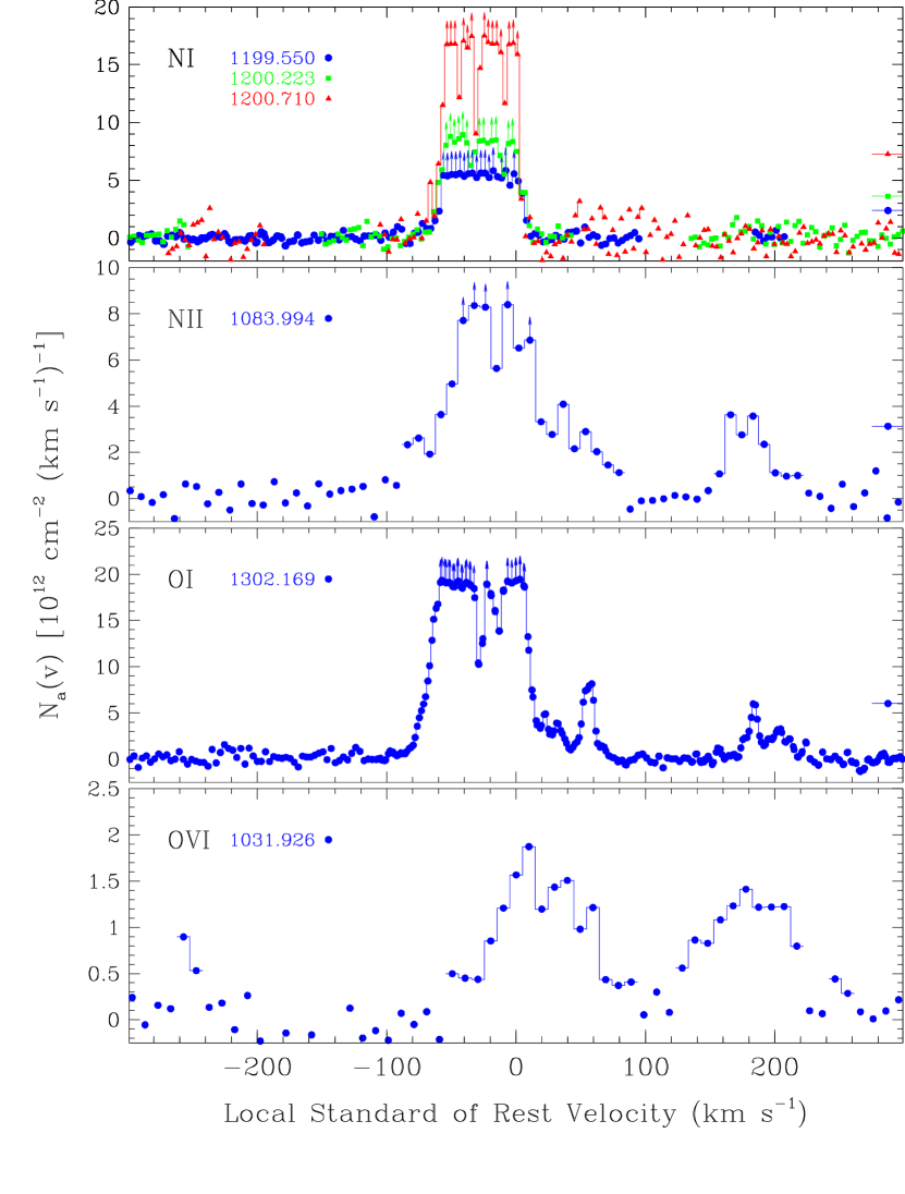
Figure 3b: Same as Figure 3a

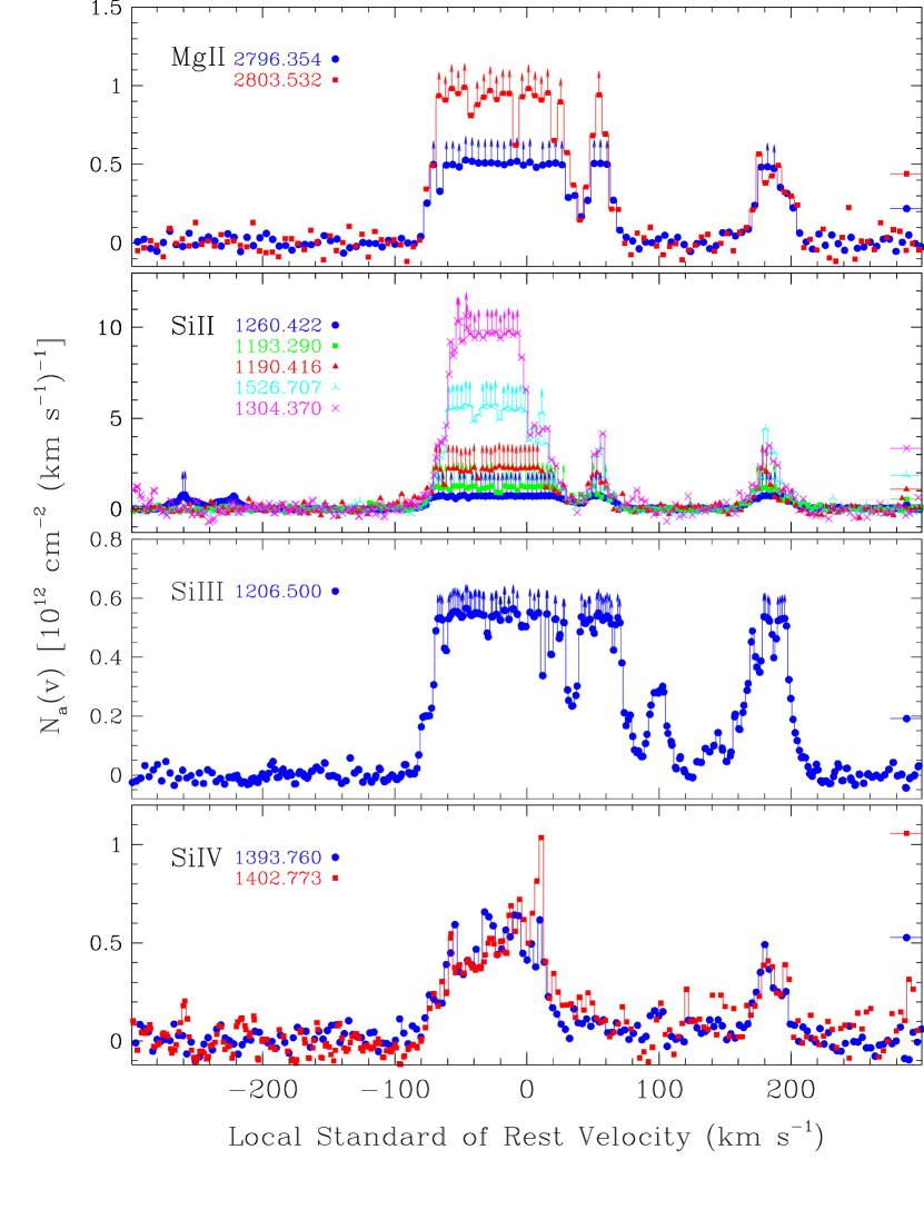
Figure 3c: Same as Figure 3a

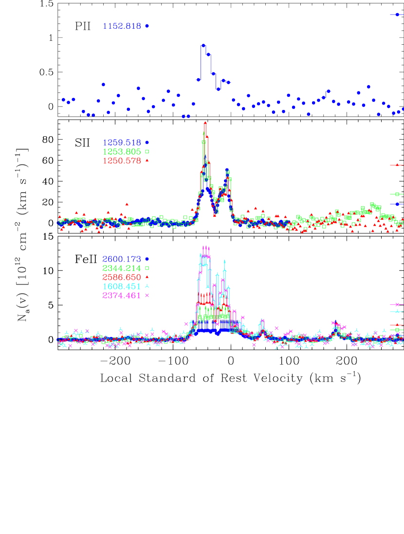
Figure 3d: Same as Figure 3a

Figure 4a: In the above panels, we show the composite apparent column density profiles of all the species detected in Galactic absorption, ordered by atomic number and ionization stage. Velocity bins where the apparent optical depth of even the weakest available transition is larger than unity are indicated with arrows. The horizontal bar in the C II panel at 250 km s^-1 indicates the velocity range of a spurious feature caused by absorption by C II* at $v<0$km s^-1. Similarly, the horizontal bar in the C III panel at -250 km s^-1 indicates the location of the O I$\lambda 976.448$ absorption which has been removed for clarity. For velocity bins where the apparent optical depth of the weakest available transition is greater than unity, we quote a lower limit on the apparent column density. See the text for a listing of transitions used in computing the profiles.

Figure 4b: Same as Figure 4a

Figure 5: In the above panels, we show the composite apparent column density profiles of the species detected in the high velocity cloud at $v_{\mathrm{LSR}}\approx+184$ km s^-1 ordered by ionization potential. Velocity bins where even the weakest available transition of a species are saturated are indicated with arrows. The horizontal bar in the top left corner of each panel gives the full-width at half-maximum intensity of the instrumental spread function. The shaded region in the O I panel marks the velocity where the absorption is blended with a weak Lyman $\alpha$ line at $z=0.0719$. Similarly, the shaded region in the C II profile marks the velocity where the absorption is blended with C II* absorption in the $v_{\mathrm{LSR}}\approx-44$ km s^-1 component.

Figure 7: This plot shows the Lyman series equivalent width measurements of the high velocity cloud ($W_{\lambda}/\lambda$ vs. $f\lambda$) from Table 2 for transitions detected in the FUSE SiC2A and LiF1A detector segments. The solid error bars indicate the 1$\sigma$ confidence uncertainties resulting from statistical and continuum placement errors. The dashed error bars indicate the additional systematic uncertainty from measuring the equivalent widths across the velocity range 140–230 km s^-1. Three curves of growth are overplotted corresponding to the best-fit curve (COG) and the two extreme cases considered in the profile fitting (L$\lambda$: lower limit from direct integration of Lyman $\lambda$ with a $b$-value of 26 km s^-1; ND: upper limit from non-detection of 21 cm emission and a $b$-value of 14.2 km s^-1).

Table 1: $v_{\rm{LSR}}\approx+100$ km s^-1 HVC Measurements

Ion	Transition	$\log f\lambda$	$\langle{v_{\rm{LSR}}}\rangle$	$b$	$\log N_{\mathrm{a}}$	$W_{\lambda}$	Integration Range
	(Å)		(km s-1)	(km s-1)	(cm-2)	(mÅ)	(km s-1)
H I	$1025.722$	$1.909$	$115.0\pm 1.6\pm 5.0$	$21.5\pm 1.0$	$14.94\pm 0.04\pm 0.08$	$178\pm 5\pm 32$	85 to 140
	$972.537$	$1.450$	$114.0\pm 2.3\pm 5.0$	$23.1\pm 1.5$	$15.31\pm 0.06\pm 0.09$	$166\pm 6\pm 31$	85 to 140
	$949.743$	$1.122$	$111.9\pm 1.5\pm 5.0$	$22.1\pm 1.1$	$15.69\pm 0.05\pm 0.08$	$164\pm 4\pm 30$	85 to 140
	$937.803$	$0.864$	$110.9\pm 1.7\pm 5.0$	$24.1\pm 0.8$	$16.00\pm 0.04\pm 0.09$	$164\pm 3\pm 30$	85 to 140
	$930.748$	$0.652$	$108.6\pm 1.6\pm 5.0$	$23.0\pm 1.0$	$16.15\pm 0.05\pm 0.09$	$161\pm 3\pm 30$	85 to 140
	$926.226$	$0.470$	$106.8\pm 1.5\pm 5.0$	$21.9\pm 0.6$	$16.21\pm 0.04\pm 0.08$	$148\pm 3\pm 26$	85 to 140
	$923.150$	$0.311$	$104.7\pm 1.3\pm 5.0$	$21.3\pm 1.0$	$16.38\pm 0.05\pm 0.09$	$145\pm 4\pm 26$	85 to 140
	$920.963$	$0.170$	$100.7\pm 1.0\pm 5.0$	$20.8\pm 0.9$	$16.53\pm 0.05\pm 0.11$	$134\pm 4\pm 25$	85 to 140
	$919.351$	$0.043$	$108.4\pm 1.4\pm 5.0$	$22.5\pm 0.8$	$16.51\pm 0.04\pm 0.08$	$135\pm 4\pm 25$	85 to 140
	$918.129$	$-0.072$	$104.0\pm 1.1\pm 5.0$	$22.4\pm 0.9$	$16.43\pm 0.04\pm 0.10$	$105\pm 7\pm 21$	85 to 140
C I	$1656.928$	$2.367$	$\cdots$	$\cdots$	$<12.99$	$<36$	$\cdots$
	$1277.245$	$2.225$	$\cdots$	$\cdots$	$<13.12$	$<17$	$\cdots$
	$945.191$	$2.157$	$\cdots$	$\cdots$	$<13.38$	$<27$	$\cdots$
	$1560.309$	$2.082$	$\cdots$	$\cdots$	$<13.17$	$<28$	$\cdots$
	$1328.833$	$2.077$	$\cdots$	$\cdots$	$<13.14$	$<18$	$\cdots$
C II	$1334.532$	$2.233$	$98.9\pm 2.8\pm 1.5$	$15.3\pm 5.0$	$13.28\pm 0.07\pm 0.08$	$31\pm 5\pm 6$	85 to 140
C II*	$1335.708$	$2.186$	$\cdots$	$\cdots$	$<12.97$	$<17$	$\cdots$
C III	$977.020$	$2.869$	$112.6\pm 1.3\pm 5.0$	$23.1\pm 0.8$	$13.71\pm 0.04\pm 0.09$	$143\pm 5\pm 28$	85 to 140
C IV	$1548.204$	$2.468$	$111.3\pm 1.1\pm 1.5$	$21.7\pm 0.7$	$13.34\pm 0.03\pm 0.04$	$73\pm 5\pm 7$	85 to 140
	$1550.781$	$2.167$	$107.3\pm 3.2\pm 1.5$	$21.2\pm 2.3$	$13.41\pm 0.09\pm 0.04$	$46\pm 9\pm 5$	85 to 140
N I	$1200.710$	$1.715$	$\cdots$	$\cdots$	$<13.66$	$<26$	$\cdots$
N II	$1083.994$	$2.080$	$\cdots$	$\cdots$	$<13.48$	$<34$	$\cdots$
N V	$1238.821$	$2.286$	$\cdots$	$\cdots$	$<12.98$	$<21$	$\cdots$
	$1242.804$	$1.985$	$\cdots$	$\cdots$	$<13.21$	$<17$	$\cdots$
O I	$1302.168$	$1.796$	$\cdots$	$\cdots$	$<13.13$	$<10$	$\cdots$
	$1304.858$	$1.795$	$\cdots$	$\cdots$	$<13.37$	$<17$	$\cdots$
O VI	$1031.926$	$2.136$	$\cdots$	$\cdots$	$13.29\pm 0.12\pm 0.15$	$20\pm 6\pm 7$	85 to 140
Mg I	$2026.477$	$2.360$	$\cdots$	$\cdots$	$<13.33$	$<74$	$\cdots$
	$1707.061$	$0.873$	$\cdots$	$\cdots$	$<14.60$	$<45$	$\cdots$
Mg II	$2796.354$	$3.236$	$\cdots$	$\cdots$	$<12.18$	$<66$	$\cdots$
	$2803.532$	$2.933$	$\cdots$	$\cdots$	$<12.55$	$<78$	$\cdots$
Si II	$1260.422$	$3.172$	$\cdots$	$\cdots$	$12.14\pm 0.11\pm 0.06$	$19\pm 5\pm 3$	85 to 140
	$1193.290$	$2.842$	$\cdots$	$\cdots$	$<12.58$	$<28$	$\cdots$
	$1190.416$	$2.541$	$\cdots$	$\cdots$	$<12.92$	$<30$	$\cdots$
	$1526.707$	$2.308$	$\cdots$	$\cdots$	$<12.86$	$<22$	$\cdots$
	$1304.370$	$2.051$	$\cdots$	$\cdots$	$<13.11$	$<17$	$\cdots$
Si III	$1206.500$	$3.294$	$103.8\pm 0.7\pm 1.5$	$18.6\pm 0.8$	$12.78\pm 0.02\pm 0.07$	$81\pm 4\pm 15$	85 to 140
Si IV	$1393.760$	$2.854$	$110.5\pm 2.5\pm 1.5$	$23.3\pm 1.5$	$12.54\pm 0.07\pm 0.08$	$28\pm 4\pm 5$	85 to 140
	$1402.773$	$2.552$	$\cdots$	$\cdots$	$<12.55$	$<15$	$\cdots$
P II	$1152.818$	$2.451$	$\cdots$	$\cdots$	$<12.85$	$<20$	$\cdots$
	$1532.533$	$0.667$	$\cdots$	$\cdots$	$<14.63$	$<27$	$\cdots$
S I	$1425.030$	$2.251$	$\cdots$	$\cdots$	$<12.59$	$<9$	$\cdots$
	$1295.653$	$2.052$	$\cdots$	$\cdots$	$<13.08$	$<16$	$\cdots$
S II	$1250.578$	$0.832$	$\cdots$	$\cdots$	$<14.32$	$<17$	$\cdots$
Fe II	$2382.765$	$2.882$	$\cdots$	$\cdots$	$<12.43$	$<45$	$\cdots$
	$2600.173$	$2.793$	$\cdots$	$\cdots$	$<12.50$	$<43$	$\cdots$
	$2344.214$	$2.427$	$\cdots$	$\cdots$	$<13.01$	$<54$	$\cdots$
	$2586.650$	$2.252$	$\cdots$	$\cdots$	$<13.10$	$<55$	$\cdots$
	$1608.451$	$1.968$	$\cdots$	$\cdots$	$<13.34$	$<31$	$\cdots$
	$2374.461$	$1.871$	$\cdots$	$\cdots$	$<13.55$	$<54$	$\cdots$
	$2260.780$	$0.742$	$\cdots$	$\cdots$	$<14.63$	$<50$	$\cdots$
	$2249.877$	$0.612$	$\cdots$	$\cdots$	$<14.62$	$<34$	$\cdots$

Table 2: ${v_{\mathrm{LSR}}}\approx+184$ km s^-1 HVC Measurements

Ion	Transition	$\log f\lambda$	$\langle{v_{\mathrm{LSR}}}\rangle$	$b$	$\log N_{\mathrm{a}}$	$W_{\lambda}$	Integration Range
	(Å)		(km s-1)	(km s-1)	(cm-2)	(mÅ)	(km s-1)
H I	$1025.722$	$1.909$	$180.2\pm 2.0\pm 5.0$	$36.3\pm 1.2$	$15.16\pm 0.04\pm 0.05$	$291\pm 6\pm 31$	140 to 230
	$972.537$	$1.450$	$177.9\pm 2.3\pm 5.0$	$33.9\pm 1.3$	$15.50\pm 0.05\pm 0.04$	$259\pm 6\pm 22$	140 to 230
	$949.743$	$1.122$	$177.4\pm 2.2\pm 5.0$	$34.0\pm 1.5$	$15.84\pm 0.05\pm 0.04$	$256\pm 7\pm 23$	140 to 230
	$937.803$	$0.864$	$175.5\pm 1.7\pm 5.0$	$32.5\pm 1.1$	$16.16\pm 0.04\pm 0.03$	$245\pm 6\pm 19$	140 to 230
	$930.748$	$0.652$	$177.0\pm 2.0\pm 5.0$	$32.2\pm 1.3$	$16.22\pm 0.04\pm 0.04$	$235\pm 6\pm 22$	140 to 230
	$926.226$	$0.470$	$178.3\pm 1.7\pm 5.0$	$29.4\pm 1.2$	$16.37\pm 0.05\pm 0.02$	$221\pm 7\pm 15$	140 to 230
	$923.150$	$0.311$	$186.2\pm 1.6\pm 5.0$	$32.1\pm 1.5$	$16.49\pm 0.05\pm 0.03$	$226\pm 6\pm 20$	140 to 230
	$920.963$	$0.170$	$184.6\pm 1.5\pm 5.0$	$29.4\pm 1.5$	$16.61\pm 0.05\pm 0.02$	$213\pm 7\pm 17$	140 to 230
	$919.351$	$0.043$	$179.6\pm 1.2\pm 5.0$	$26.3\pm 1.4$	$16.75\pm 0.05\pm 0.02$	$199\pm 8\pm 12$	140 to 230
	$918.129$	$-0.072$	$182.5\pm 1.6\pm 5.0$	$27.6\pm 1.7$	$16.73\pm 0.06\pm 0.02$	$183\pm 11\pm 12$	140 to 230
C I	$1656.928$	$2.367$	$\cdots$	$\cdots$	$<13.09$	$<46$	$\cdots$
	$1277.245$	$2.225$	$\cdots$	$\cdots$	$<13.24$	$<22$	$\cdots$
	$945.191$	$2.157$	$\cdots$	$\cdots$	$<13.55$	$<38$	$\cdots$
	$1560.309$	$2.082$	$\cdots$	$\cdots$	$<13.30$	$<35$	$\cdots$
	$1328.833$	$2.077$	$\cdots$	$\cdots$	$<13.23$	$<23$	$\cdots$
C II	$1334.532$	$2.233$	$192.3\pm 0.7\pm 1.5$	$22.8\pm 0.7$	$14.55\pm 0.03\pm 0.01$	$261\pm 5\pm 9$	140 to 230
	$1335.708$	$2.186$	$\cdots$	$\cdots$	$<13.08$	$<22$	$\cdots$
C III	$977.020$	$2.869$	$174.9\pm 1.5\pm 5.0$	$30.8\pm 1.3$	$13.94\pm 0.03\pm 0.03$	$225\pm 8\pm 19$	140 to 230
C IV	$1548.204$	$2.468$	$178.3\pm 1.9\pm 1.5$	$21.6\pm 2.4$	$13.74\pm 0.04\pm 0.01$	$153\pm 12\pm 3$	140 to 230
	$1550.781$	$2.167$	$183.7\pm 3.2\pm 1.5$	$22.7\pm 3.8$	$13.70\pm 0.06\pm 0.01$	$82\pm 11\pm 1$	140 to 230
N I	$1200.223$	$2.018$	$\cdots$	$\cdots$	$<13.47$	$<32$	$\cdots$
	$1200.710$	$1.715$	$\cdots$	$\cdots$	$<13.72$	$<34$	$\cdots$
N II	$1083.994$	$2.080$	$181.0\pm 2.6\pm 5.0$	$24.7\pm 2.4$	$14.25\pm 0.06\pm 0.01$	$117\pm 14\pm 3$	140 to 230
N V	$1238.821$	$2.286$	$\cdots$	$\cdots$	$<13.10$	$<27$	$\cdots$
	$1242.804$	$1.985$	$\cdots$	$\cdots$	$<13.32$	$<22$	$\cdots$
O I	$1302.168$	$1.796$	$192.8\pm 1.3\pm 1.5$	$22.0\pm 1.9$	$14.12\pm 0.02\pm 0.01$	$75\pm 4\pm 2$	140 to 230
			$180.2\pm 1.4\pm 1.5$	$11.9\pm 3.5$	$13.82\pm 0.03\pm 0.07$	$37\pm 3\pm 7$	140 to 192
O I*	$1304.858$	$1.795$	$\cdots$	$\cdots$	$<13.46$	$<21$	$\cdots$
O VI	$1031.926$	$2.136$	$182.2\pm 2.1\pm 5.0$	$32.7\pm 1.5$	$14.00\pm 0.03\pm 0.02$	$99\pm 7\pm 4$	140 to 230
Mg I	$2026.477$	$2.360$	$\cdots$	$\cdots$	$<13.43$	$<96$	$\cdots$
	$1707.061$	$0.873$	$\cdots$	$\cdots$	$<14.71$	$<63$	$\cdots$
Mg II	$2796.354$	$3.236$	$184.4\pm 1.4\pm 2.5$	$16.5\pm 2.2$	$13.19\pm 0.06\pm 0.01$	$319\pm 26\pm 8$	140 to 230
	$2803.532$	$2.933$	$186.2\pm 3.0\pm 2.5$	$14.3\pm 6.0$	$13.17\pm 0.07\pm 0.01$	$208\pm 33\pm 6$	140 to 230
Si II	$1260.422$	$3.172$	$184.6\pm 0.6\pm 1.5$	$17.4\pm 0.8$	$13.50\pm 0.03\pm 0.01$	$185\pm 6\pm 6$	140 to 230
	$1193.290$	$2.842$	$185.0\pm 1.4\pm 1.5$	$17.9\pm 2.0$	$13.59\pm 0.05\pm 0.01$	$145\pm 10\pm 1$	140 to 230
	$1190.416$	$2.541$	$178.5\pm 2.7\pm 1.5$	$4.2\pm 21.0$	$13.56\pm 0.08\pm 0.01$	$71\pm 12\pm 3$	140 to 230
	$1526.707$	$2.308$	$184.8\pm 1.3\pm 1.5$	$11.9\pm 3.4$	$13.82\pm 0.04\pm 0.01$	$108\pm 8\pm 2$	140 to 230
	$1304.370$	$2.051$	$179.7\pm 2.0\pm 1.5$	$8.7\pm 7.7$	$13.85\pm 0.04\pm 0.01$	$68\pm 7\pm 2$	140 to 230
Si III	$1206.500$	$3.294$	$181.4\pm 0.6\pm 1.5$	$20.8\pm 0.6$	$13.37\pm 0.02\pm 0.01$	$193\pm 4\pm 6$	140 to 230
Si IV	$1393.760$	$2.854$	$181.0\pm 1.5\pm 1.5$	$23.6\pm 1.9$	$13.07\pm 0.03\pm 0.01$	$82\pm 6\pm 3$	140 to 230
	$1402.773$	$2.552$	$179.7\pm 2.8\pm 1.5$	$28.3\pm 2.6$	$13.15\pm 0.05\pm 0.03$	$55\pm 6\pm 3$	140 to 230
P II	$1152.818$	$2.451$	$\cdots$	$\cdots$	$<13.03$	$<29$	$\cdots$
	$1532.533$	$0.667$	$\cdots$	$\cdots$	$<14.75$	$<36$	$\cdots$
S I	$1425.030$	$2.251$	$\cdots$	$\cdots$	$<12.69$	$<11$	$\cdots$
	$1295.653$	$2.052$	$\cdots$	$\cdots$	$<13.19$	$<21$	$\cdots$
S II	$1250.578$	$0.832$	$\cdots$	$\cdots$	$<14.46$	$<21$	$\cdots$
Fe II	$2382.765$	$2.882$	$185.5\pm 1.4\pm 2.5$	$20.0\pm 2.0$	$13.41\pm 0.04\pm 0.01$	$240\pm 18\pm 4$	140 to 230
	$2600.173$	$2.793$	$182.7\pm 1.4\pm 2.5$	$14.8\pm 2.9$	$13.41\pm 0.05\pm 0.01$	$186\pm 18\pm 11$	140 to 230
	$2344.214$	$2.427$	$\cdots$	$\cdots$	$13.36\pm 0.09\pm 0.02$	$92\pm 22\pm 7$	140 to 230
	$2586.650$	$2.252$	$\cdots$	$\cdots$	$13.47\pm 0.10\pm 0.03$	$88\pm 23\pm 9$	140 to 230
	$1608.451$	$1.968$	$\cdots$	$\cdots$	$<13.49$	$<39$	$\cdots$
	$2374.461$	$1.871$	$\cdots$	$\cdots$	$<13.70$	$<71$	$\cdots$
	$2260.780$	$0.742$	$\cdots$	$\cdots$	$<14.73$	$<63$	$\cdots$
	$2249.877$	$0.612$	$\cdots$	$\cdots$	$<14.73$	$<45$	$\cdots$

Table 3: Galactic Halo and Intermediate-Velocity Gas Measurements

Ion	Transition	$\log f\lambda$	$\langle{v_{\mathrm{LSR}}}\rangle$	$b$	$\log N_{\mathrm{a}}$	$W_{\lambda}$	Integration Range
	(Å)		(Å)	(km s-1)	(cm-2)	(mÅ)	(km s-1)
H I	$930.748$	$0.652$	$5.2\pm 3.0\pm 5.0$	$75.2\pm 1.8$	$16.63\pm 0.03\pm 0.02$	$524\pm 6\pm 27$	-100 to 85
	$926.226$	$0.470$	$3.6\pm 3.1\pm 5.0$	$70.5\pm 1.8$	$16.83\pm 0.03\pm 0.02$	$515\pm 7\pm 22$	-100 to 85
	$923.150$	$0.311$	$6.6\pm 3.5\pm 5.0$	$70.6\pm 2.1$	$16.96\pm 0.03\pm 0.02$	$509\pm 8\pm 21$	-100 to 85
	$920.963$	$0.170$	$8.9\pm 3.4\pm 5.0$	$70.2\pm 2.1$	$17.11\pm 0.03\pm 0.03$	$501\pm 9\pm 21$	-100 to 85
	$919.351$	$0.043$	$-0.3\pm 3.9\pm 5.0$	$69.7\pm 2.3$	$17.21\pm 0.03\pm 0.01$	$505\pm 9\pm 18$	-100 to 85
	$918.129$	$-0.072$	$-11.9\pm 3.7\pm 5.0$	$72.2\pm 2.4$	$17.38\pm 0.03\pm 0.02$	$532\pm 8\pm 28$	-100 to 85
C I	$1656.932$	$2.367$	$\cdots$	$\cdots$	$<13.29$	$<73$	$\cdots$
	$1277.245$	$2.225$	$\cdots$	$\cdots$	$<13.38$	$<34$	$\cdots$
	$945.191$	$2.157$	$\cdots$	$\cdots$	$<13.71$	$<53$	$\cdots$
	$1560.309$	$2.082$	$\cdots$	$\cdots$	$<13.47$	$<55$	$\cdots$
	$1328.833$	$2.077$	$\cdots$	$\cdots$	$<13.44$	$<42$	$\cdots$
C II	$1334.532$	$2.233$	$-2.6\pm 1.5\pm 1.5$	$59.8\pm 1.0$	$15.04\pm 0.02\pm 0.01$	$666\pm 6\pm 7$	-100 to 85
C III	$977.020$	$2.869$	$3.9\pm 2.0\pm 5.0$	$66.4\pm 1.4$	$14.33\pm 0.02\pm 0.01$	$508\pm 8\pm 20$	-100 to 85
C IV	$1548.204$	$2.468$	$-12.2\pm 1.9\pm 1.5$	$58.6\pm 1.5$	$14.17\pm 0.02\pm 0.01$	$401\pm 14\pm 5$	-100 to 85
	$1550.781$	$2.167$	$-14.3\pm 3.9\pm 1.5$	$61.3\pm 3.2$	$14.17\pm 0.03\pm 0.01$	$234\pm 18\pm 3$	-100 to 85
N I	$1199.550$	$2.200$	$-29.4\pm 1.7\pm 1.5$	$29.2\pm 3.0$	$14.67\pm 0.03\pm 0.01$	$282\pm 14\pm 1$	-100 to 85
	$1200.710$	$1.715$	$-26.1\pm 1.9\pm 1.5$	$30.9\pm 3.2$	$15.08\pm 0.03\pm 0.01$	$247\pm 17\pm 4$	-100 to 85
N II	$1083.994$	$2.080$	$-9.0\pm 2.8\pm 5.0$	$59.6\pm 2.3$	$14.88\pm 0.03\pm 0.01$	$411\pm 19\pm 6$	-100 to 85
N V	$1238.821$	$2.286$	$\cdots$	$\cdots$	$<13.14$	$<31$	$\cdots$
	$1242.804$	$1.985$	$\cdots$	$\cdots$	$<13.48$	$<33$	$\cdots$
O I	$1302.168$	$1.796$	$-21.2\pm 0.8\pm 1.5$	$46.5\pm 0.7$	$15.24\pm 0.01\pm 0.01$	$467\pm 5\pm 2$	-100 to 85
O VI	$1031.926$	$2.136$	$18.5\pm 4.0\pm 5.0$	$42.2\pm 6.6$	$14.16\pm 0.03\pm 0.01$	$136\pm 14\pm 1$	-100 to 85
Mg I	$2026.477$	$2.360$	$\cdots$	$\cdots$	$<13.59$	$<180$	$\cdots$
	$1707.061$	$0.873$	$\cdots$	$\cdots$	$<14.86$	$<89$	$\cdots$
Mg II	$2796.354$	$3.236$	$-7.6\pm 2.6\pm 2.5$	$57.1\pm 1.8$	$13.90\pm 0.03\pm 0.01$	$1218\pm 32\pm 2$	-100 to 85
	$2803.532$	$2.933$	$-9.5\pm 2.8\pm 2.5$	$55.9\pm 2.0$	$14.11\pm 0.03\pm 0.01$	$1091\pm 38\pm 3$	-100 to 85
Si II	$1260.422$	$3.172$	$-7.6\pm 1.7\pm 1.5$	$57.9\pm 1.2$	$14.03\pm 0.02\pm 0.01$	$598\pm 7\pm 4$	-100 to 85
	$1193.290$	$2.842$	$-10.2\pm 2.2\pm 1.5$	$55.0\pm 1.6$	$14.25\pm 0.02\pm 0.01$	$501\pm 12\pm 2$	-100 to 85
	$1190.416$	$2.541$	$-17.9\pm 2.5\pm 1.5$	$56.8\pm 2.1$	$14.44\pm 0.03\pm 0.01$	$465\pm 15\pm 4$	-100 to 85
	$1526.707$	$2.308$	$-18.7\pm 1.3\pm 1.5$	$45.4\pm 1.2$	$14.71\pm 0.02\pm 0.01$	$525\pm 10\pm 1$	-100 to 85
	$1304.370$	$2.051$	$-21.8\pm 0.9\pm 1.5$	$42.9\pm 1.2$	$14.95\pm 0.02\pm 0.01$	$427\pm 8\pm 4$	-100 to 85
Si III	$1206.500$	$3.294$	$-0.3\pm 1.3\pm 1.5$	$61.6\pm 0.8$	$13.92\pm 0.01\pm 0.01$	$590\pm 5\pm 6$	-100 to 85
Si IV	$1393.760$	$2.854$	$-18.9\pm 1.3\pm 1.5$	$48.6\pm 1.5$	$13.68\pm 0.01\pm 0.01$	$293\pm 8\pm 2$	-100 to 85
	$1402.773$	$2.552$	$-9.5\pm 1.9\pm 1.5$	$43.9\pm 2.5$	$13.71\pm 0.02\pm 0.01$	$182\pm 7\pm 4$	-100 to 85
P II	$1152.818$	$2.451$	$-25.5\pm 8.5\pm 5.0$	$43.2\pm 13.3$	$13.59\pm 0.08\pm 0.01$	$76\pm 15\pm 1$	-100 to 85
	$1532.533$	$0.667$	$\cdots$	$\cdots$	$<14.74$	$<41$	$\cdots$
S I	$1425.030$	$2.251$	$\cdots$	$\cdots$	$<12.84$	$<18$	$\cdots$
	$1295.653$	$2.052$	$\cdots$	$\cdots$	$<13.41$	$<34$	$\cdots$
S II	$1250.578$	$0.832$	$-38.9\pm 3.0\pm 1.5$	$49.6\pm 4.5$	$15.49\pm 0.03\pm 0.03$	$167\pm 10\pm 11$	-100 to 85
Fe II	$2382.765$	$2.882$	$-12.4\pm 2.2\pm 2.5$	$55.7\pm 1.6$	$14.13\pm 0.02\pm 0.01$	$924\pm 23\pm 3$	-100 to 85
	$2600.173$	$2.793$	$-13.3\pm 1.7\pm 2.5$	$51.7\pm 1.4$	$14.22\pm 0.02\pm 0.01$	$966\pm 23\pm 10$	-100 to 85
	$2344.214$	$2.427$	$-21.2\pm 1.7\pm 2.5$	$42.0\pm 1.9$	$14.55\pm 0.03\pm 0.01$	$760\pm 28\pm 3$	-100 to 85
	$2586.650$	$2.252$	$-23.9\pm 1.9\pm 2.5$	$38.6\pm 2.3$	$14.61\pm 0.04\pm 0.01$	$689\pm 29\pm 6$	-100 to 85
	$1608.451$	$1.968$	$-27.5\pm 1.8\pm 1.5$	$40.1\pm 2.6$	$14.79\pm 0.03\pm 0.01$	$373\pm 16\pm 2$	-100 to 85
	$2374.461$	$1.871$	$-28.4\pm 2.2\pm 2.5$	$40.8\pm 3.3$	$14.86\pm 0.03\pm 0.01$	$513\pm 30\pm 7$	-100 to 85
	$2260.780$	$0.742$	$-21.1\pm 7.9\pm 2.5$	$44.5\pm 12.0$	$15.16\pm 0.06\pm 0.01$	$134\pm 23\pm 3$	-100 to 85
	$2249.877$	$0.612$	$\cdots$	$\cdots$	$15.04\pm 0.11\pm 0.03$	$73\pm 24\pm 5$	-100 to 85

Table 4: Adopted Column Densities

	$\log[N~{}(\mathrm{cm}^{-2})]$
Ion	$-44$ km s-1	$-7$ km s-1	$+56$ km s-1	$100$ km s-1	$184$ km s-1
C I	$13.23\pm 0.08$	$<12.87$	$<12.80$	$<12.83$	$<12.94$
C II	$>14.56$	$>14.68$	$>14.39$	$13.28\pm 0.07$	$>14.55$
C III	$>13.78$	$>13.88$	$>13.77$	$>13.71$	$>13.94$
C IV	$13.77\pm 0.03$	$13.82\pm 0.03$	$13.36\pm 0.05$	$13.34\pm 0.03$	$13.74\pm 0.04$
N I	$>14.75$	$>14.79$	$<13.65$	$<13.66$	$<13.47$
N II	$>14.44$	$>14.54$	$14.11\pm 0.06$	$<13.48$	$>14.25$
N V	$<12.78$	$<12.84$	$<12.91$	$<12.91$	$<13.10$
O I	$>14.92$	$>14.91$	$>14.06$	$<13.13$	$13.82_{-0.03}^{+0.09}$
O VI	$<13.24$	$13.94\pm 0.03$	$13.65\pm 0.06$	$13.29\pm 0.12$	$14.00\pm 0.03$
Mg I	$<13.43$	$<13.47$	$<13.06$	$<13.33$	$<13.43$
Mg II	$>13.70$	$>13.76$	$>13.20$	$<12.18$	$13.18\pm 0.05$
Si II	$>14.64$	$>14.60$	$>13.74$	$12.14\pm 0.11$	$13.85\pm 0.04$
Si III	$>13.45$	$>13.53$	$>13.35$	$>12.78$	$>13.37$
Si IV	$13.27\pm 0.01$	$13.37\pm 0.02$	$12.58\pm 0.05$	$12.54\pm 0.07$	$13.09_{-0.03}^{+0.06}$
P II	$13.38\pm 0.10$	$13.07\pm 0.10$	$<12.95$	$<12.85$	$<13.03$
S I	$<12.62$	$<12.59$	$<12.55$	$<12.59$	$<12.69$
S II	$>15.12$	$14.95\pm 0.03$	$<13.94$	$<14.32$	$<14.46$
Fe II	$14.92\pm 0.06$	$14.68\pm 0.11$	$13.30\pm 0.03$	$<12.43$	$13.46\pm 0.09$

Table 5: Column Density Ratios and Relative Abundance Constraints for High Ionization Species

Model/Component	$N_{\mathrm{a}}$(Si IV)/$N_{\mathrm{a}}$(O VI)	$N_{\mathrm{a}}$(C IV)/$N_{\mathrm{a}}$(O VI)	$N_{\mathrm{a}}$(N V)/$N_{\mathrm{a}}$(O VI)
IVC @ ${v_{\mathrm{LSR}}}\approx-44$ km s-1	$>1.07$	$>3.39$	$\cdots$
ISM @ ${v_{\mathrm{LSR}}}\approx-7$ km s-1	$0.27\pm 0.02$	$0.76\pm 0.07$	$<0.08$
IVC @ ${v_{\mathrm{LSR}}}\approx+56$ km s-1	$0.09\pm 0.02$	$0.51\pm 0.09$	$<0.18$
HVC @ ${v_{\mathrm{LSR}}}\approx+100$ km s-1	$0.17\pm 0.05$	$1.12\pm 0.25$	$<0.42$
HVC @ ${v_{\mathrm{LSR}}}\approx+184$ km s-1	$0.12\pm 0.01$	$0.55\pm 0.06$	$<0.11$
Radiative Cooling	0.001–0.013	0.036–0.170	0.053–0.090
Conductive Interfaces	0.003–0.058	0.042–0.930	0.065–0.510
Turbulent Mixing Layers	0.087–1.290	1.050–6.920	0.170–0.580
Shock Ionization	0.002–0.180	0.016–1.040	0.031–0.051

Table 6: Model Parameters for Lyman Series Fit

Velocity	$b$(H I)	$\log N$(H I)	$b$(O I)	$\log N$(O I)
(km s-1)	(km s-1)	(cm-2)	(km s-1)	(cm-2)
$-43.6\pm 0.5$	$15.5$	$19.83$	$12.7\pm 0.1$	$16.49$
$-8.2\pm 0.8$	$14.7$	$19.70$	$8.8\pm 0.1$	$16.36$
$26.7\pm 1.0$	$37.0\pm 3.1$	$17.29$	$13.0\pm 3.8$	$13.95\pm 0.07$
$55.93\pm 0.07$	$9.9\pm 0.3$	$17.58$	$3.8\pm 0.2$	$14.24\pm 0.02$
$100$	$21.9\pm 1.7$	$16.42\pm 0.02$	$\cdots$	$\cdots$
$z=0.0719$	$9.6\pm 1.53$	$12.81\pm 0.04$	$\cdots$	$\cdots$
$183.3\pm 0.2$	$\begin{array}[]{c}25.9\pm 0.6\\ 14.2\pm 0.1\end{array}$	$\begin{array}[]{c}16.73\tablenotemark{b}\\ 18.3\tablenotemark{b}\end{array}$	$3.9\pm 0.3$	$13.82$

Table 7: Adopted Solar Abundances

Element	A⊙	Reference
C	8.39	Allende Prieto et al. (2002)
N	7.931	Holweger (2001)
O	8.66	Asplund et al. (2004)
Mg	7.538	Holweger (2001)
Al	6.48	Anders & Grevesse (1989)
Si	7.536	Holweger (2001)
P	5.57	Anders & Grevesse (1989)
S	7.27	Anders & Grevesse (1989)
Fe	7.448	Holweger (2001)

Table 8: Logarithmic Column Density Ratios

Sight line	PKS $2155-304$		Mrk 509
Ratio/Velocity	–140 km s-1	–270 km s-1	–240 km s-1	–300 km s-1	Complex C
$N_{\mathrm{a}}$(H I)/$N_{\mathrm{a}}$(O VI)	$2.57_{-0.14}^{+0.22}$	$1.67_{-0.23}^{+0.38}$	$<3.80$	$<3.76$	$6.38_{-0.05}^{+0.05}$
$N_{\mathrm{a}}$(O I)/$N_{\mathrm{a}}$(O VI)	$<-0.40$	$<-0.05$	$<-0.42$	$<-0.31$	$2.15\pm 0.14$
$N_{\mathrm{a}}$(Si II)/$N_{\mathrm{a}}$(Si IV)	$0.07_{-0.13}^{+0.14}$	$<0.51$	$\cdots$	$<-0.31$	$2.03_{-0.20}^{+0.22}$
$N_{\mathrm{a}}$(C II)/$N_{\mathrm{a}}$(C IV)	$0.36_{-0.08}^{+0.11}$	$<-0.56$	$<-0.38$	$-0.47_{-0.06}^{+0.06}$	$\cdots$
$N_{\mathrm{a}}$(C IV)/$N_{\mathrm{a}}$(Si IV)	$0.74_{-0.09}^{+0.08}$	$1.30_{-0.16}^{+0.12}$	$>1.04$	$0.78_{-0.07}^{+0.06}$	$0.59_{-0.15}^{+0.12}$
$N_{\mathrm{a}}$(C IV)/$N_{\mathrm{a}}$(N V)	$>0.40$	$>0.47$	$>0.45$	$>0.94$	$>0.07$
$N_{\mathrm{a}}$(O VI)/$N_{\mathrm{a}}$(C IV)	$0.32_{-0.05}^{+0.05}$	$0.00_{-0.07}^{+0.06}$	$0.36_{-0.07}^{+0.06}$	$-0.25_{-0.06}^{+0.05}$	$0.31_{-0.09}^{+0.08}$
Sight line	HE $0226-4110$		PG $0953+414$
Ratio/Velocity	+145 km s-1	+200 km s-1	+120 km s-1
$N_{\mathrm{a}}$(H I)/$N_{\mathrm{a}}$(O VI)	$2.99\pm 0.27$	$<3.16$	$3.01\pm 0.23$
$N_{\mathrm{a}}$(O I)/$N_{\mathrm{a}}$(O VI)	$<0.19$	$<0.30$	$<0.61$
$N_{\mathrm{a}}$(Si II)/$N_{\mathrm{a}}$(Si IV)	$>0.28$	$-0.27\pm 0.16$	$<0.21$
$N_{\mathrm{a}}$(C II)/$N_{\mathrm{a}}$(C IV)	$0.66\pm 0.14$	$0.67\pm 0.19$	$>0.41$
$N_{\mathrm{a}}$(C IV)/$N_{\mathrm{a}}$(Si IV)	$>1.04$	$0.31\pm 0.24$	$0.84\pm 0.33$
$N_{\mathrm{a}}$(C IV)/$N_{\mathrm{a}}$(N V)	$>0.06$	$>0.20$	$>-0.19$
$N_{\mathrm{a}}$(O VI)/$N_{\mathrm{a}}$(C IV)	$0.10\pm 0.14$	$>-0.19$	$0.09\pm 0.21$
Sight Line	PG $1116+215$
Ratio/Velocity	–44 km s-1	–7 km s-1	+56 km s-1	+100 km s-1	+184 km s-1
$N_{\mathrm{a}}$(H I)/$N_{\mathrm{a}}$(O VI)	$>6.59$	$5.77\pm 0.03$	$\cdots$	$3.13\pm 0.012$	$3.82\pm 0.18$
$N_{\mathrm{a}}$(O I)/$N_{\mathrm{a}}$(O VI)	$>1.68$	$>0.97$	$>0.41$	$<-0.16$	$-0.18_{-0.04}^{+0.09}$
$N_{\mathrm{a}}$(Si II)/$N_{\mathrm{a}}$(Si IV)	$>1.37$	$>1.23$	$>1.16$	$-0.40\pm 0.13$	$0.76\pm 0.07$
$N_{\mathrm{a}}$(C II)/$N_{\mathrm{a}}$(C IV)	$>0.79$	$>0.86$	$>1.03$	$-0.06\pm 0.08$	$>0.81$
$N_{\mathrm{a}}$(C IV)/$N_{\mathrm{a}}$(Si IV)	$0.50\pm 0.03$	$0.45\pm 0.04$	$0.78\pm 0.07$	$0.80\pm 0.08$	$0.65\pm 0.07$
$N_{\mathrm{a}}$(C IV)/$N_{\mathrm{a}}$(N V)	$>0.99$	$>0.98$	$>0.45$	$>0.43$	$>0.64$
$N_{\mathrm{a}}$(O VI)/$N_{\mathrm{a}}$(C IV)	$<-0.53$	$0.12\pm 0.04$	$0.29\pm 0.08$	$-0.05\pm 0.12$	$0.26\pm 0.05$

Table 9: Cloud Key

Number	Sight Line	Velocity	Gal. Long.	Gal. Lat.
		(km s-1)	(∘)	(∘)
1	PG $1116+215$	$-44$	$223\fdg 36$	$+68\fdg 21$
2	PG $1116+215$	$-7$	$223\fdg 36$	$+68\fdg 21$
3	PG $1116+215$	$+56$	$223\fdg 36$	$+68\fdg 21$
4	PG $1116+215$	$+100$	$223\fdg 36$	$+68\fdg 21$
5	PG $1116+215$	$+184$	$223\fdg 36$	$+68\fdg 21$
6	HE $0226-4110$	$+145$	$253\fdg 94$	$-65\fdg 77$
7	HE $0226-4110$	$+200$	$253\fdg 94$	$-65\fdg 77$
8	PG $0953+414$	$+120$	$179\fdg 79$	$+51\fdg 71$
9	PKS $2155-304$	$-140$	$17\fdg 73$	$-52\fdg 25$
10	PKS $2155-304$	$-270$	$17\fdg 73$	$-52\fdg 25$
11	Mrk 509	$-240$	$35\fdg 97$	$-29\fdg 86$
12	Mrk 509	$-300$	$35\fdg 97$	$-29\fdg 86$
13	PG $1259+593$	$-110$	$120\fdg 56$	$+58\fdg 05$

References

- Allende Prieto et al. (2002) Allende Prieto, C., Lambert, D. L., & Asplund, A. 2002, ApJ, 573, 137
- Anders & Grevesse (1989) Anders, E., & Grevesse, N. 1989, Geochim. Cosmochim. Acta, 53, 197
- Asplund et al. (2004) Asplund, M., Grevesse, N., Sauval, A., Allende Prieto, C., & Kiselman, D. 2004, A&A, in press (astro-ph/0312290)
- Bland-Hawthorn & Maloney (1999) Bland-Hawthorn, J., & Maloney, P. R. 1999, ApJ, 510, L33
- Bland-Hawthorn & Maloney (2001) Bland-Hawthorn, J., & Maloney, P. R. 2001, ApJ, 550, L231
- Bland-Hawthorn & Putman (2001) Bland-Hawthorn, J., & Putman, M. E. 2001, in ASP Conf. Ser. 240: Gas and Galaxy Evolution, ed. J. E. Hibbard, M. Rupen, & J. H. van Gorkom, 369
- Blitz et al. (1999) Blitz, L., Spergel, D. N., Teuben, P. J., Hartmann, D., & Burton, W. B. 1999, ApJ, 514, 818
- Borkowski et al. (1990) Borkowski, K. J., Balbus, S. A., & Fristrom, C. C. 1990, ApJ, 355, 501
- Collins et al. (2003) Collins, J. A., Shull, J. M., & Giroux, M. L. 2003, ApJ, 585, 336
- Collins et al. (2004a) Collins, J. A., Shull, J. M., & Giroux, M. L. 2004a, ApJ, submitted
- Collins et al. (2004b) Collins, J. A., Shull, J. M., & Giroux, M. L. 2004b, ApJ, in press (astro-ph/0312105)
- Dopita & Sutherland (1996) Dopita, M. A., & Sutherland, R. S. 1996, ApJS, 102, 161
- Ferland (2001) Ferland, G. J. 2001, Hazy, a brief introduction to Cloudy 94.00
- Field & Steigman (1971) Field, G. B., & Steigman, G. 1971, ApJ, 166, 59
- Fox et al. (2004) Fox, A. J., Savage, B. D., Wakker, B. P., Richter, P., Sembach, K. R., & Tripp, T. M. 2004, ApJ, 602, 738
- Fox et al. (2005) Fox, A. J., Savage, B. D., Wakker, B. P., Tripp, T. M., & Sembach, K. R. 2005, ApJ, in preparation
- Haardt & Madau (1996) Haardt, F., & Madau, P. 1996, ApJ, 461, 20
- Heckman et al. (2002) Heckman, T. M., Norman, C. A., Strickland, D. K., & Sembach, K. R. 2002, ApJ, 577, 691
- Holweger (2001) Holweger, H. 2001, in AIP Conf. Proc. 598: Joint SOHO/ACE workshop “Solar and Galactic Composition”, ed. R. F. Wimmer-Schweingruber (Bern: AIP), 23
- Indebetouw & Shull (2004) Indebetouw, R., & Shull, J. M. 2004, ApJ, 607, 309
- Jenkins & Tripp (2001) Jenkins, E. B., & Tripp, T. M. 2001, ApJS, 137, 297
- Kimble et al. (1998) Kimble, R. A., et al. 1998, in Proc. SPIE Vol. 3356, p. 188-202, Space Telescopes and Instruments V, Pierre Y. Bely; James B. Breckinridge; Eds., 188
- Kuntz & Danly (1996) Kuntz, K. D., & Danly, L. 1996, ApJ, 457, 703
- Lu et al. (1998) Lu, L., Sargent, W. L. W., Savage, B. D., Wakker, B. P., Sembach, K. R., & Oosterloo, T. A. 1998, AJ, 115, 162
- Mihalas & Binney (1981) Mihalas, D., & Binney, J. 1981, Galactic astronomy: Structure and kinematics (2nd edition) (San Francisco, CA, W. H. Freeman and Co., 1981. 608 p.)
- Moos et al. (2000) Moos, H. W., et al. 2000, ApJ, 538, L1
- Morras et al. (2000) Morras, R., Bajaja, E., Arnal, E. M., & Pöppel, W. G. L. 2000, A&AS, 142, 25
- Morton (2003) Morton, D. C. 2003, ApJS, 149, 205
- Murray & Lin (2004) Murray, S. D., & Lin, D. N. C. 2004, ApJ, in press (astro-ph/0407411)
- Nicastro et al. (2002) Nicastro, F., et al. 2002, ApJ, 573, 157
- Nicastro et al. (2003) Nicastro, F., et al. 2003, Nature, 421, 719
- Oegerle et al. (2004) Oegerle, W. R., Jenkins, E. B., Shelton, R., Bowen, D. V., & Chayer, P. 2004, ApJ, submitted
- Press et al. (1992) Press, W. H., Teukolsky, S. A., Vetterling, W. T., & Flannery, B. P. 1992, Numerical recipes in C. The art of scientific computing (Cambridge: University Press, 1992, 2nd ed.)
- Proffitt et al. (2002) Proffitt, C., et al. 2002, STIS Intrument Handbook, Version 6.0 (Baltimore: STScI)
- Putman et al. (1998) Putman, M. E., et al. 1998, Nature, 394, 752
- Quilis & Moore (2001) Quilis, V., & Moore, B. 2001, ApJ, 555, L95
- Rosenberg et al. (2003) Rosenberg, J. L., Ganguly, R., Giroux, M. L., & Stocke, J. T. 2003, ApJ, 591, 677
- Sahnow et al. (2000) Sahnow, D. J., et al. 2000, ApJ, 538, L7
- Savage et al. (1994) Savage, B. D., Sembach, K. R., & Cardelli, J. A. 1994, ApJ, 420, 183
- Savage et al. (1997) Savage, B. D., Sembach, K. R., & Lu, L. 1997, AJ, 113, 2158
- Savage et al. (2003) Savage, B. D., et al. 2003, ApJS, 146, 125
- Schneider et al. (1993) Schneider, D. P., et al. 1993, ApJS, 87, 45
- Scott et al. (2002) Scott, J., Bechtold, J., Morita, M., Dobrzycki, A., & Kulkarni, V. P. 2002, ApJ, 571, 665
- Sembach et al. (2001a) Sembach, K. R., Howk, J. C., Savage, B. D., & Shull, J. M. 2001a, AJ, 121, 992
- Sembach et al. (2001b) Sembach, K. R., Howk, J. C., Savage, B. D., Shull, J. M., & Oegerle, W. R. 2001b, ApJ, 561, 573
- Sembach & Savage (1992) Sembach, K. R., & Savage, B. D. 1992, ApJS, 83, 147
- Sembach et al. (1999) Sembach, K. R., Savage, B. D., Lu, L., & Murphy, E. M. 1999, ApJ, 515, 108
- Sembach et al. (1997) Sembach, K. R., Savage, B. D., & Tripp, T. M. 1997, ApJ, 480, 216
- Sembach et al. (2004a) Sembach, K. R., Tripp, T. M., Savage, B. D., & Richter, P. 2004a, ApJS, in press (Dec.)
- Sembach et al. (2003) Sembach, K. R., et al. 2003, ApJS, 146, 165
- Sembach et al. (2004b) Sembach, K. R., et al. 2004b, ApJS, 150, 387
- Slavin et al. (1993) Slavin, J. D., Shull, J. M., & Begelman, M. C. 1993, ApJ, 407, 83
- Stocke et al. (2004) Stocke, J. T., Keeney, B. A., McLin, K. M., Rosenberg, J. L., Weymann, R. J., & Giroux, M. L. 2004, ApJ, 609, 94
- Tripp et al. (2001) Tripp, T. M., Giroux, M. L., Stocke, J. T., Tumlinson, J., & Oegerle, W. R. 2001, ApJ, 563, 724
- Tripp et al. (2002) Tripp, T. M., et al. 2002, ApJ, 575, 697
- Tripp et al. (1998) Tripp, T. M., Lu, L., & Savage, B. D. 1998, ApJ, 508, 200
- Tripp & Savage (2000) Tripp, T. M., & Savage, B. D. 2000, ApJ, 542, 42
- Tripp et al. (2003) Tripp, T. M., et al. 2003, AJ, 125, 3122
- Wakker (2001) Wakker, B. P. 2001, ApJS, 136, 463
- Wakker (2004a) Wakker, B. P. 2004a, Ap&SS, 289, 381
- Wakker (2004b) Wakker, B. P. 2004b, ApJ, in press
- Wakker et al. (2003) Wakker, B. P., et al. 2003, ApJS, 146, 1
- Weiner et al. (2002) Weiner, B. J., Vogel, S. N., & Williams, T. B. 2002, in ASP Conf. Ser. 254: Extragalactic Gas at Low Redshift, ed. J. S. Mulchaey & J. Stocke, 256
- Welty et al. (1999) Welty, D. E., Frisch, P. C., Sonneborn, G., & York, D. G. 1999, ApJ, 512, 636
- Welty et al. (1997) Welty, D. E., Lauroesch, J. T., Blades, J. C., Hobbs, L. M., & York, D. G. 1997, ApJ, 489, 672
- Woodgate et al. (1998) Woodgate, B. E., et al. 1998, PASP, 110, 1183