Environmental Impact on the Southeast Limb of the Cygnus Loop

Abstract

We analyze observations from the Chandra X-ray Observatory of the southeast knot of the Cygnus Loop supernova remnant. In this region, the blast wave propagates through an inhomogeneous environment. Extrinsic differences and subsequent multiple projections along the line of sight rather than intrinsic shock variations, such as fluid instabilities, account for the apparent complexity of the images. Interactions between the supernova blast wave and density enhancements of a large interstellar cloud can produce the morphological and spectral characteristics. Most of the X-ray flux arises in such interactions, not in the diffuse interior of the supernova remnant. Additional observations at optical and radio wavelengths support this account of the existing interstellar medium and its role in shaping the Cygnus Loop, and they demonstrate that the southeast knot is not a small cloud that the blast wave has engulfed. These data are consistent with rapid equilibration of electron and ion temperatures behind the shock front, and the current blast wave velocity $v_{bw}\approx 330{\rm\,km\,s^{-1}}$. Most of this area does not show strong evidence for non-equilibrium ionization conditions, which may be a consequence of the high densities of the bright emission regions.

1 Introduction

Supernova remnants play a fundamental role in processing matter and energy in galaxies. Supernovae create the heaviest elements, and their remnants mix the enriched ejecta into the surrounding interstellar medium (ISM). Supernova remnants (SNRs) are the primary source of the hot component of the ISM, and the supernova rate, with the remnants’ subsequent evolution, determines whether this component predominates in any particular galaxy. The extant environment reciprocally affects the evolution of a SNR. If large, dense clouds populate the surroundings with large covering fraction, the blast wave’s expansion will stall, limiting the amount of thermal energy that is injected into the ISM.

The Cygnus Loop is a middle-aged ($8,000$ years old) supernova remnant, now interacting with large-scale inhomogeneities in the surrounding ISM. These variations are responsible for its observable characteristics, including a limb-brightened X-ray shell and strong correlations between X-ray and optical surface brightness. Propagating through the low-density environment its progenitor evacuated, the undisturbed blast wave has a velocity $v_{s}\approx 350{\rm\,km\,s^{-1}}$ and produces low surface brightness X-ray emission with temperature $kT\approx 0.15$ keV ($T\approx 1.8\times 10^{6}$ K). Upon encountering a large, dense cloud, however, the blast wave is decelerated, to $v_{s}<200{\rm\,km\,s^{-1}}$. The post-shock material rapidly cools through optical line emission to $T\approx 10^{4}$ K. An important consequence of the cloud interaction is the development of reflected shocks. These shocks propagate back through the hot, compressed interior of the SNR, enhancing X-ray emission (Hester & Cox, 1986).

The northeastern and western limbs of the Cygnus Loop offer two clear examples of these interactions between shock fronts and large clouds (Hester, Raymond, & Blair, 1994; Levenson, Graham, & Walters, 2002). Although less prominent than these bright regions, the southeast knot is physically similar. Fesen, Kwitter, & Downes (1992) first drew attention to this feature, and subsequent work by Graham et al. (1995) demonstrated that it represents the early stage of the encounter between the blast wave and a large interstellar cloud. The southeast knot is also located near a portion of the primary blast wave traced in H$\alpha$ at optical wavelengths. These are “nonradiative” shocks, which excite Balmer line emission through electron collisions in unshocked gas that is predominantly neutral (Chevalier & Raymond, 1978). Thus, they identify sites where the gas is being shocked for the first time. The shocked gas has not yet had time to cool radiatively, so the optical spectra lack the emission lines that are typical of fully radiative post-shock regions, such as [O III] and [S II], in addition to the Balmer lines.

The Cygnus Loop is nearby and bright, allowing high spatial resolution and high signal-to-noise observations to investigate variations and shock evolution on physically-relevant scales. At the 440 pc distance of this SNR (Blair et al., 1999), $1\arcsec$ corresponds to a physical size of $6.6\times 10^{15}$ cm. Here we analyze new observations of the Cygnus Loop’s southeast knot obtained with the Chandra X-ray Observatory (Chandra). In addition to superb spatial resolution, Chandra also provides simultaneous spectroscopic information for direct and unambiguous measurement of the distinct physical character of different areas. Combining these X-ray data with previous optical and radio measurements, we distinguish temporal evolution of the post-shock medium from external variations in the environment.

The three-dimensional geometry of the Cygnus Loop complicates the interpretation of observations. Multiple projections of the current blast wave location or cloud interactions can emerge along a single line of sight. As a result, areas that appear projected onto the interior of the SNR may actually represent newly-shocked material that is located in the foreground (or background), not older shocked gas that is genuinely inside the hot SNR interior. In the southeast, we illustrate that many of the observed variations are a consequence of these projection effects.

2 Observations and Data Reduction

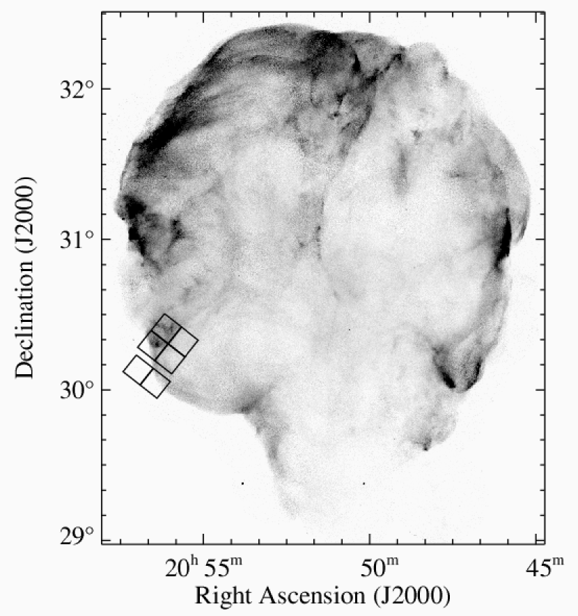
Figure 1: ACIS field of view overlaid on mosaic of ROSAT HRI soft X-ray image (Levenson et al., 1997, completed with later observations).

We observed the southeast knot of the Cygnus Loop with the Chandra Advanced CCD Imaging Spectrometer (ACIS) on 2000 September 1, obtaining spatial resolution around $1\arcsec$ over energy $E=0.3$–$8$ keV, and simultaneous spectral resolution $E/\Delta E\approx 12$. The total field of view of the six CCDs is approximately $25\arcmin\times 17\arcmin$ and covers the brightest X-ray region of the southeast knot, some of the diffuse interior, and some slight X-ray enhancements close to the blast wave. Figure 1 illustrates these observations in the context of the Cygnus Loop as a whole. The bright southeast knot is at the apex of a slight indentation from the near-circular boundary of the SNR. Five of the CCDs (I0, I1, I2, I3, and S2) are front-illuminated (FI), having readout electronics that face the incident photons. The sole back-illuminated (BI) CCD, S3, is located entirely outside the blast wave boundary. Because the sensitivity of the BI and FI CCDs is different, the S3 data are not useful for measuring background emission, so we will not discuss them.

We reprocessed all data from original Level 1 event files using Chandra Interactive Analysis of Observations (CIAO) software, version 3.1, removing the 0.5-pixel spatial randomization that is included in standard processing. (See the Chandra Science Center for details about Chandra data and standard processing procedures.) We applied current calibrations (Calibration Database version 2.28), including corrections for charge-transfer inefficiency and time-dependent gain variations, to produce the Level 2 event file. We included only good events that do not lie on node boundaries, where discrimination of cosmic rays is difficult. We examined the lightcurves of background regions and found no significant flares, so we did not reject any additional data from the standard good-time intervals, for a net exposure of 47 ks.

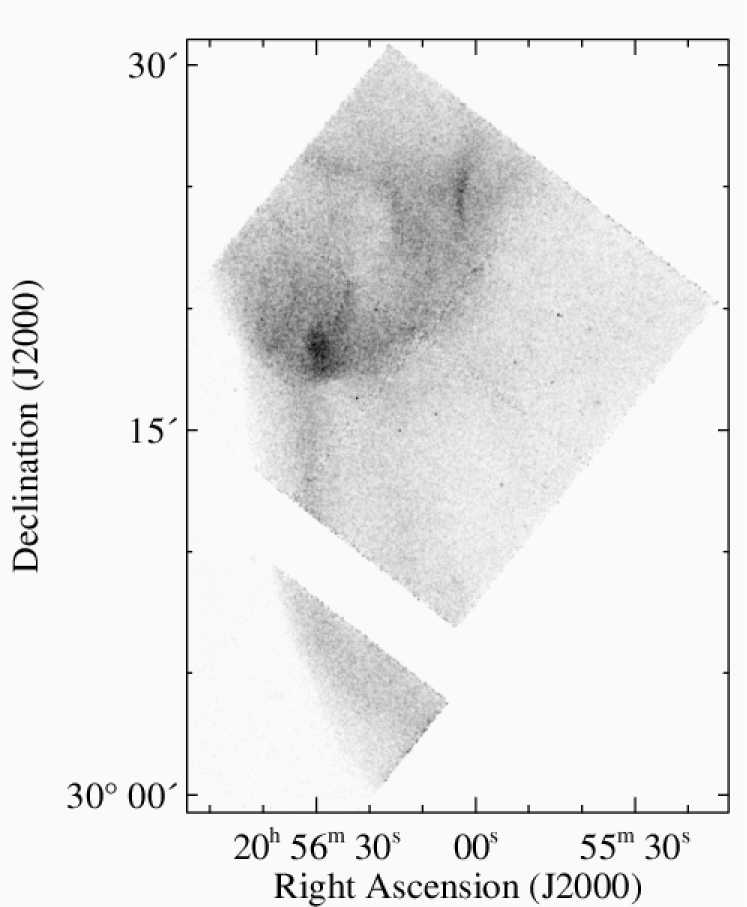
Figure 2: Total (0.3–8 keV) exposure-corrected image, scaled linearly from 0 (white) to $7\times 10^{-7}{\rm\,photons\,cm^{-2}\,arcsec^{-2}}$ (black). The large gap that separates the four northern ACIS detectors from the southernmost one is unobserved.

We created exposure maps to correct soft (0.3–0.6 keV), medium (0.6–0.9 keV), hard (0.9–2 keV), and very hard (2–8 keV) images separately. The total exposure-corrected image (Figure 2) includes all these bands, with the raw pixels binned by a factor of two (to 1 arcsec²) and smoothed by a Gaussian of FWHM=5$\arcsec$. Spacecraft dither during the exposure is sufficient to cover the small gaps among the four northern CCDs, but a large gap separating the southern CCD remains unobserved.

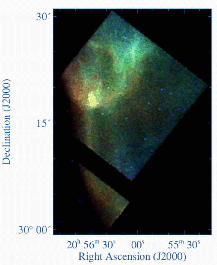
Figure 3: False-color image, constructed from soft (red; 0.3–0.6 keV), medium (green; 0.6–0.9 keV), and hard (blue; 0.9–2 keV) exposure-corrected images. The individual images have been smoothed by a Gaussian of FWHM=5$\arcsec$ and scaled linearly, from 0 to 4, 1, and 0.3 $\times 10^{-7}{\rm\,photons\,cm^{-2}\,arcsec^{-2}}$, respectively.

Spectral variations are apparent in a false-color image constructed from the three softer bands (Figure 3). Nearly all the emission above 2 keV is due to background point sources unlikely to be related to the SNR, and many of these hard sources are evident in the blue band of the color image. The emission near the blast wave is generally soft, and the low surface brightness interior is harder. Stronger hard emission also arises near the site of interaction with the dense southeast cloud.

3 Spectral Modeling

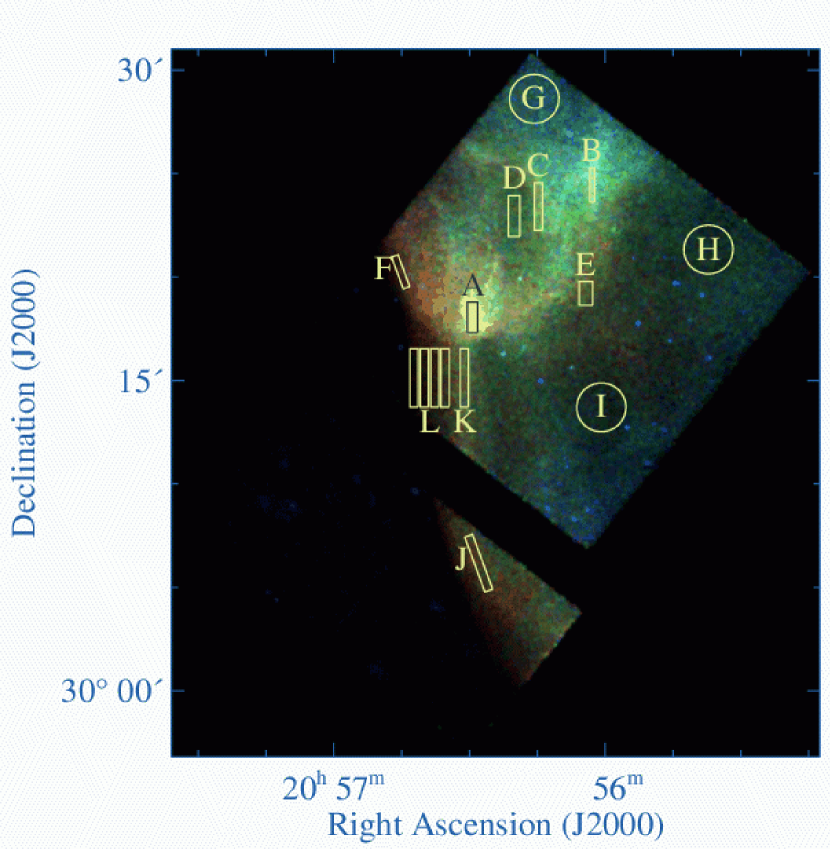
Figure 4: Spectroscopic apertures are identified on the false-color Chandra image.

We select regions for spectral analysis from the color image, identifying extended areas of distinct spectral character. Figure 4 shows these locations. The regions are not of uniform size or shape, in order to isolate unique physical characteristics within each aperture. The spatially-limited spectral extractions require specific processing and calibration measurements. As we noted above, we applied corrections for the charge-transfer inefficiency and gain variations that have developed over time in creating the Level 2 events file. Another significant change over the course of the Chandra mission is the reduced soft X-ray sensitivity, likely the result of build-up of material on the detector. In constructing ancillary response files, we used the CIAO contamination correction to account for this variation in quantum efficiency.

Because the Cygnus Loop covers nearly the entire field of view, we measure the background emission in comparable observations of the blank sky. The blank sky background spectra have been filtered and processed the same way as the data, and scaled by the relative exposure time. A portion of the I3 and S2 detectors covers the exterior of the SNR. We compared local background measurements for source spectra within these detectors and found no significant difference from the blank-sky backgrounds. For consistency, we use the blank-sky background measurements in all cases.

We fit the spectra in XSPEC (Arnaud, 1996), grouping the spectra into bins of a minimum of 20 counts, so the errors are normally distributed and $\chi^{2}$ statistics are appropriate. We use data from 0.5 keV (below which the calibration becomes uncertain) to 2.0 keV, the maximum energy of any significant emission. In general, we expect to find thermal emission behind the blast wave of this SNR. We use the collisional ionization equilibrium models of Borkowski et al. (Hamilton, Chevalier, & Sarazin, 1983; Borkowski, Sarazin, & Blondin, 1994; Liedahl et al., 1995), including dielectronic recombination rates of Mazzotta et al. (1998), the VEQUIL model in XSPEC.

We consider abundance variations, which we quote relative to solar values of Anders & Grevesse (1989). At the typical temperature of this area of the Cygnus Loop, oxygen and iron produce the strongest emission lines. While groups of elements may be expected to vary the same way if they are produced through the same modes of stellar evolution—with other alpha elements similar to oxygen and other iron group elements similar to iron—other members of these nucleosynthetic families are in fact not at all significant in the observed spectra. Therefore, we do not include their variation in the spectral modeling.

Oxygen is the only element whose abundance differs from the solar value, and it is consistently underabundant relative to the Anders & Grevesse (1989) value of $(O/H)_{\sun}=8.51\times 10^{4}$. Our findings are more typical of the local ISM, however. Within 500 pc of the Sun, Meyer, Jura, & Cardelli (1998), for example, find gas-phase $(O/H)=3.43\times 10^{4}$, correcting for updated transition probabilities (Welty et al., 1999, cited in André et al. 2003).

Some spectra demand more complex models to attain adequate fits, requiring additional temperature components or non-equilibrium conditions. In the more complex models that are presented, the inclusion of additional model components and their free parameters are significant at a minimum of the 95% confidence limit, based on an $F$-test. All quoted errors are 90% confidence for one parameter of interest. Figures 5 and 6 show two example spectra and their corresponding equilibrium model fits on the same scale.

3.1 Equilibrium Results

All single-temperature equilibrium model fits are listed in Table 1, with the values of $\chi^{2}$ and the number of degrees of freedom (dof) in the last column. This model yields the best fits in regions B, D, E, and K. In these regions, the single-temperature equilibrium plasmas have temperatures $kT=0.17$–$0.19$ keV and sub-solar oxygen abundance. These regions are generally associated with the southeast knot and located near the shocked cloud’s optical emission. We discuss these spectral results in the context of this inhomogeneous environment below (§5), after considering more complex models.

Regions G, H, and I require two thermal components, listed in Table 2. The same foreground column density is applied to both components. These apertures are located in the diffuse interior of the SNR, and they are not directly associated with interactions between the blast wave and the southeast cloud or the cavity boundary. These areas are noticeably bluer in the energy-coded color image. Each of these regions is fit with a soft component similar to the single-temperature regions, as well as a hotter ($kT_{2}\approx 0.6$–$0.7$ keV) component. Qualitatively, we recognize that these apertures cover material that was heated by the passage of the original undisturbed blast wave, before it was strongly decelerated in an encounter with higher-density material. At each location, shocked SNR material extends along the line of sight, representing a range of original shock velocities. In the two-temperature model, however, neither component quantitatively reveals consistent adiabatic evolution of the blast wave. We attempted to fit these spectra with a model that explicitly accounts for this evolution (the VSEDOV model), but the resulting fits are worse.

4 Non-Equilibrium Conditions

4.1 Non-Equilibrium Ionization

In addition to the equilibrium descriptions above, we also examined non-equilibrium conditions that may be relevant in the Cygnus Loop. One important consideration is the ionization state relative to the electron temperature. Initially, the post-shock gas is underionized compared with its equilibrium value. In the spectrum, the temperature the lines indicate, based on ionization state, then differs from the continuum temperature, which the electrons determine. The ionization timescale, $\tau=n_{e}t$, parameterizes the degree of equilibration in terms of $n_{e}$, the electron density, and $t$, the time elapsed since the shock passage (Gorenstein, Tucker, & Harnden, 1974). The timescale for ionization equilibrium varies for each element and is a function of temperature. For example, at $T=2.0\times 10^{6}$ K ($kT=0.17$ keV), the ionization equilibration $e$-folding timescale for oxygen $t_{ieq}\approx 3\times 10^{11}n_{e}^{-1}$ s (Liedahl, 1999; Shull & van Steenberg, 1982).

Globally, we do not expect the interior of the Cygnus Loop to be in ionization equilibrium, with $\tau\approx 3\times 10^{10}{\rm\,cm^{-3}\,s}$ for $n\approx 0.1{\rm\,cm^{-3}}$ and an age of 8,000 years. However, the brightest emission is produced in cloud interactions at much higher densities, and are therefore more likely to be equilibrated. At the southeast, the fainter (and therefore lower density) edge regions, in which the elapsed time is also shorter, are most likely to be out of ionization equilibrium. In the present observations, non-equilibrium planar shock models (the VPSHOCK model in XSPEC) improve the spectral fits of regions A, C, F, and J compared with the corresponding equilibrium models. In these cases, we include the integrated contribution from the time of initial shock ($\tau_{i}=0$), and fit for the current value of the ionization timescale. These results are listed in Table 3, and Figure 7 illustrates the non-equilibrium ionization example of the region F spectrum.

Regions A and C are not strongly out of equilibrium, with upper limits of $\tau\approx 5\times 10^{12}{\rm\,cm^{-3}\,s}$. The non-equilibrium effects are stronger in the lower surface brightness (and therefore likely lower density) regions F and J. The best-fitting temperature of region J is unphysically high, corresponding to an equilibrium shock velocity $v_{s}=500{\rm\,km\,s^{-1}}$, but it is not constrained well. The uncertainties encompass temperatures that are more typical of the southeast Cygnus Loop ($kT\sim 0.17$ keV).

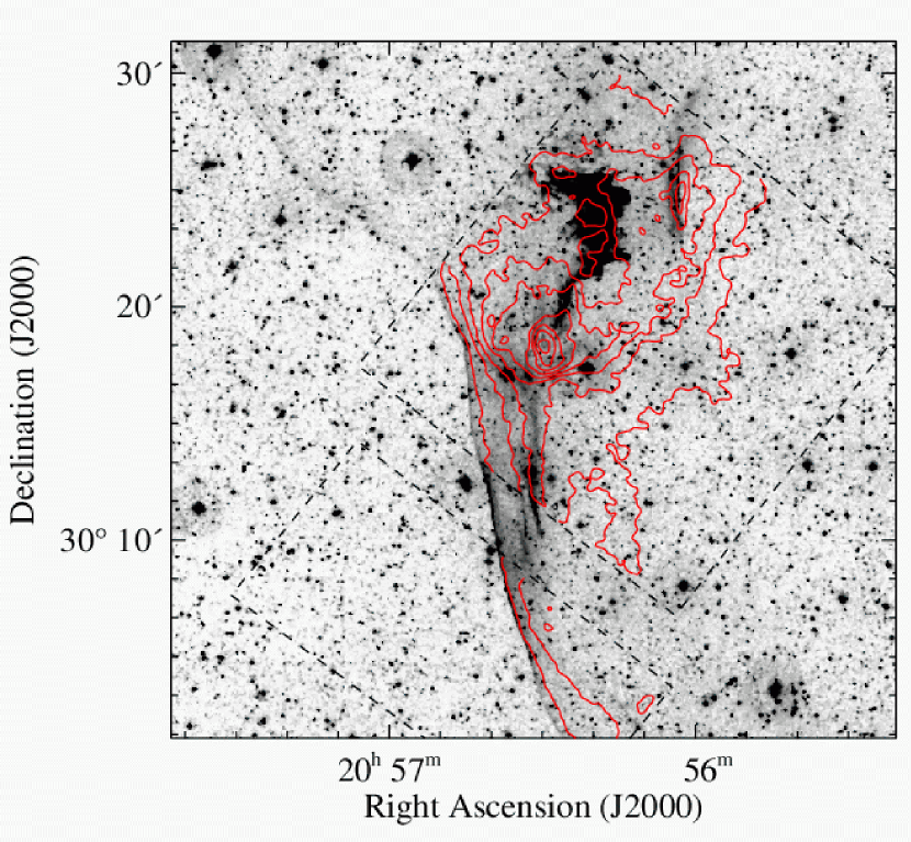
Figure 8: Chandra total-band contours overlaid on the H$\alpha$ image of the southeast knot (from Levenson et al., 1998). The optical image is scaled logarithmically, and the X-ray contours are linear. Dashed lines mark the boundary of the ACIS field of view. The brightest X-ray emission (Region A) is located south of the optically-bright cloud. The X-ray enhancement of Region B is coincident with a radiative shock. The narrow H$\alpha$ filaments toward the exterior of the SNR mark the boundary of the blast wave.

In an effort to measure changes in the emission behind the shock front and evolution toward equilibrium, we examined the spectra near the edge of the SNR. The Balmer-dominated filaments directly reveal the current (projected) location of the blast wave. The region around $\alpha=20^{\rm h}56^{\rm m}40^{\rm s},\delta=30^{\circ}15\arcmin 10\arcsec$ offers the clearest signature, with a bright Balmer filament marking the shock front (Figure 8). These filaments are not curved, and this region has no other indication of complicating projection effects over nearly 2′ toward the SNR’s interior, where another nonradiative filament is apparent.

We extracted spectra from four regions located at incrementally increasing distance behind the blast wave (L1–L4). The regions are relatively narrow ($24\arcsec\equiv 1.6\times 10^{17}$ cm) and extend 170″ parallel to the shock front. We considered fitting the spectra individually and together, to explicitly follow the evolution toward equilibrium of the shocked material. In fitting the spectra jointly, we constrained the column density, abundance, and equilibrium temperature to be the same in all cases. The upper bound on ionization timescale is a free parameter for each region, and this value served as the lower bound on $\tau$ for the adjacent interior region. We allowed the normalization to vary independently in the four spectra.

The non-equilibrium models do not improve the spectral fits in any case. The independent fits tend toward equilibrium, with $\tau\geq 10^{12}{\rm\,cm^{-3}\,s}$. Furthermore, in both the independent and the combined fits, the ionization parameter does not vary smoothly behind the blast wave. These results are surprising because the time since shock passage is minimized and the densities are not necessarily extremely high at these edge regions, so non-equilibrium conditions would seem likely. The faintness of the easternmost regions may preclude significant measurement of their genuine non-equilibrium conditions. The equilibrium models do show systematic temperature variation from the edge to the interior, which we discuss in terms of electron-ion temperature disequilibrium or shock deceleration.

4.2 Electron-Ion Temperature Disequilibrium

Immediately following the passage of a strong shock, all particles acquire the same velocity distribution. Because their masses are different, electrons and protons are initially heated to different temperatures. The temperatures equilibrate through Coulomb collisions in the post-shock region. However, plasma instabilities may promote rapid equilibration at the shock front (Cargill & Papadopoulos, 1988).

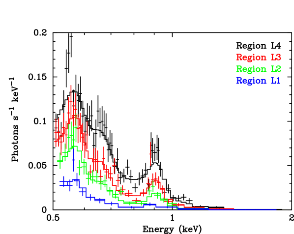
Figure 9: ACIS spectra (crosses) of regions L1 through L4. Region L1 (blue) is located $2\times 10^{17}$ cm behind the blast wave. Regions L2, L3, and L4 (green, red, and black, respectively) are each offset a further $2\times 10^{17}$ cm behind the preceding region. The column density and abundance are the same in all regions, while temperature and normalization vary in the ionization equilibrium models (histograms). The observed temperature gradient is inconsistent with Coulomb collisions alone to equilibrate the electron and ion temperatures behind the shock front.

To investigate the role of collisionless equilibration, we examine the variation of the electron temperature behind the shock front in the spectra of regions L1–L4. Although we do not measure the ion temperature, it has little direct effect on these spectra. Similar to the combined fits above, we simultaneously fit the spectra of regions L1–L4 with the VEQUIL model (Figure 9), constraining the column density and abundance to be the same in all cases while allowing the temperature and normalization to be free parameters. A single-temperature plasma model provides a reasonable fit, with sub-solar oxygen abundance and low foreground column density (Table 4). The results are not significantly different from the independent fits of these regions (Table 1), but applying the common column density and abundance is more appropriate in this interpretation of the evolution of a single shock front.

Similar to the independent equilibrium fits of these four spectra, we find a gradual temperature gradient increasing toward the interior of the SNR. In detail, however, these measurements disagree with the predictions of Coulomb equilibration alone. For a simple comparison, we use the observed Balmer filament to define the location of the blast wave, and the interior $kT=0.17$ keV yields the equilibrium electron temperature. In terms of $T_{i}$, the ion temperature, the electron temperature evolves

$${dT_{e}\over dt}={T_{i}-T_{e}\over t_{eq}(T_{e},T_{i})}$$

(Spitzer, 1940, cited in Spitzer 1962). The timescale, $t_{eq}$, is inversely proportional to density, and for $n=0.1{\rm\,cm^{-3}}$, $t_{eq}\approx 10^{11}$ s as equilibrium $T_{e}=1.9\times 10^{6}$ K is approached. Assuming the interior region L4 is fully equilibrated, we use its temperature to determine the shock velocity ($v_{s}=360{\rm\,km\,s^{-1}}$), and we then relate the elapsed time to the observable post-shock distances. For $n=0.1{\rm\,cm^{-3}}$ and Coulomb equilibration alone, we would expect $kT=0.05$ keV near the edge, and a maximum of only 0.09 keV at the innermost location. This theoretical prediction sharply contrasts the observed higher temperatures and their more gradual rise.

One reasonable concern is that an equilibrium model is used to determine the electron temperature of each of the regions, while nonequilibrium ionization would be expected to influence the effective temperatures we measure. Over most of the range of timescales and temperatures we observe, however, the majority of the line emission is due to O VII transitions. The absence of higher ionization states does not strongly alter these spectra. Other indications of non-equilibrium, such as diagnostic line ratios, cannot be distinguished at the present low spectral resolution, so they do not drive the spectral fitting. Furthermore, as described above, the non-equilibrium ionization models empirically fail to provide a physically reasonable description of the data. Finally and most significantly, the net effect of non-equilibrium ionization would be to increase the measured temperatures, requiring yet more rapid temperature equilibration.

Considering the uncertainties in the temperature measurements, Coulomb equilibration could be marginally consistent if the density were very high ($n=2{\rm\,cm^{-3}}$). However, the observed flux precludes such a large density. The $0.4\times 3.0{\rm\,pc^{2}}$ region L1 is offset $26\arcsec$ to the interior of the blast wave. The nearly-spherical SNR has a radius of $84\arcmin$, so the line of sight through shocked material at the location of L1 is $6.8\times 10^{18}$ cm. From the observed emission of this volume, we find $n=0.1{\rm\,cm^{-3}}$. The Coulomb equilibration model assumes constant density over the shocked region, yet region L1 is most likely the highest density of the four areas. It is located at the boundary of the cavity that surrounded the progenitor rather than in the evacuated interior. We therefore conclude that Coulomb equilibration is insufficient to produce the observed variation of electron temperature as a function of distance behind the shock front, and rapid post-shock equilibration is required.

These results agree with other observations of similar shocks elsewhere in the Cygnus Loop, where the initial ion and electron temperatures are fully equilibrated (Ghavamian et al., 2001; Raymond et al., 2003). In general, equilibration appears to decrease with increasing shock velocity (Raymond et al., 2003; Rakowski, Ghavamian, & Hughes, 2003). The blast wave of the Cygnus Loop is relatively slow, in contrast to faster shocks of younger SNRs, which do show significant temperature disequilibrium between electrons and ions (e.g., Raymond, Blair, & Long, 1995; Laming et al., 1996).

The overall decline in temperature toward the SNR’s boundary may be a consequence of global blast wave deceleration in the surrounding material. This shell contrasts with the rarefied bubble that the progenitor evacuated, through which the blast wave had propagated previously. This blast wave deceleration is a genuine dynamical effect, not merely electron-ion temperature disequilibrium, and it has been observed around the entire rim of the Cygnus Loop (Levenson et al., 1998). Adopting the equilibrium temperature found in region L1 at the edge yields a current blast wave velocity $v_{bw}=330(+12,-17){\rm\,km\,s^{-1}}$. This value is somewhat lower than the shock velocity of the nearby interior region, L4. A single, abrupt step of density contrast 1.4 could produce this velocity ratio in the two regions.

5 Interpretation

Data from ROSAT demonstrate that the southeast knot is the result of interaction of the supernova blast wave with a large-scale interstellar cloud (Graham et al., 1995). Here the X-ray rim is indented from the near-circular boundary that can be traced over most of the SNR’s periphery (Figure 1). Preventing any portion of the projected blast wave edge from reaching this circular boundary requires a large obstacle that extends parsecs along the line of sight to impede the blast wave. During the early stages of the encounter, X-ray emission increases near the interaction site, a consequence of pressure enhancement when a reflected shock propagates back through the previously shocked and compressed SNR interior. If the speed of the forward shock propagating through the cloud remains high, the increased density in the cloud shock may also enhance X-ray emission.

The small size of the optical southeast knot mistakenly led Fesen et al. (1992) and Klein, McKee, & Colella (1994) to envision a physically small, engulfed cloud. This early work also misinterpreted an optical feature (near region B) as the Mach disk that develops after the blast wave has passed. As Graham et al. (1995) show, however, the shock front propagates through a significantly neutral, and therefore unshocked medium here. This analysis—combined with the location of the X-ray enhancement west of the optical emission, which requires that the blast wave propagate east—demonstrates that the optical feature cannot be the Mach disk.

These Chandra observations further support the basic interpretation of the southeast knot as the early stage of interaction between the blast wave and a large-scale cloud. A small, engulfed cloud would not produce the extended and significant X-ray enhancements that are observed interior of the optical cloud, and the Mach disk would not be so luminous. Also, material stripped from such a cloud would not generate the bright X-rays toward the exterior at a similar temperature. We interpret the present results in the context of interactions with the large cloud and dense material located at the boundary of the SNR.

While a large obstacle is present, the X-ray spectral variations indicate that its surface is not uniform. The X-ray emission shows significant multiple projections on sub-parsec scales, similar to the very small scale structure within the optical knot that high-resolution optical images show (Levenson & Graham, 2001). Regions B and C are sites at the immediate edges the cloud-shock interaction, with increased X-ray emission located adjacent to the optical emission of cloud shocks.

Spectrally, Region C is hotter than nearly all the other regions fit with a single-temperature model, independent of whether the equilibrium or non-equilibrium results are adopted. Because of the confusion along the line of sight in the diffuse interior (regions H and I, especially), region L4 offers the best measurement of the undisturbed blast wave for comparison. It is cooler than region C, with $kT=0.17$ keV. At region C, the greater intensity combined with higher temperature is consistent with the hotter contribution due to a reflected shock. This characteristic temperature increase would not be observed during the late stage of interaction (after the blast wave has completely engulfed a cloud). A second component of the early interaction, the forward shock that propagates through the dense cloud, is not directly detected in the spectrum, likely because the shock front is rapidly decelerated below X-ray-emitting temperatures. However, this immediate interaction site does include a softer component that appears as mottled red patches in the color image. These soft X-rays within aperture C contrast with the exclusively hotter material that extends to the west, evident as a bright blue/green area. Spectrally we find $kT=0.193\pm 0.005$ keV in the western area, without much emission below 0.6 keV.

In region B, we would also expect to find evidence of the hotter reflected shock or, if the eastward-moving cloud shock remains fast enough, the continuation of the slower forward shock. Surprisingly, the spectrum of region B does not exhibit a high temperature similar to region C. It is somewhat but not significantly hotter than region L4. The column density measured at B is higher than that of all other regions fit with single-temperature equilibrium models. The temperature does increase ($kT=0.181\pm 0.004$ keV) if the column density is fixed at a value more typical of the surrounding areas ($1\times 10^{20}{\rm\,cm^{-2}}$), but the fit is worse ($\chi^{2}/\nu=116/69$). Alternatively, a weaker hot component ($kT=0.20$ keV) may be included in addition to the dominant $kT=0.18$ keV component and high column density, but it does not significantly improve the fit. Without definitive spectral identification, the X-ray morphology and the association with optical emission provide the strongest evidence that region B represents the interaction between the blast wave and a facet of the large interstellar cloud that is obvious at optical wavelengths. The narrow area of high surface brightness distinguishes region B from the diffuse SNR interior or a projected edge of the undisturbed blast wave. This interaction interpretation contrasts alternative accounts of this feature as either the Mach disk of a prior shock or the emission from a dense shell that the SNR swept up while propagating through the homogeneous ISM.

Region D is coincident with the optical cloud, in which shocks are slowed to $v_{s}<200{\rm\,km\,s^{-1}}$ and therefore do not produce X-rays. This region shows little or no additional intrinsic absorption, so the X-ray-emitting region is likely located in the foreground of the cloud along the same line of sight. The volume of hot gas is therefore smaller than the full line of sight through the SNR, resulting in a lower surface brightness.

The highest surface brightness area we observe is region A, yet a single-temperature model fits the spectrum well. (As in region C, the non-equilibrium results are similar and do not strongly rule out equilibrium conditions.) Here multiple projections can account for the increased flux, with a greater column of hot gas located along a single line of sight. This bright spot is located near the apex of two nonradiative shocks. The Balmer filaments mark two separate projections of the blast wave, each appearing when the curved blast wave is viewed at a tangency, through a long line of sight, so we expect the X-ray surface brightness to double behind them. The observed surface brightness is increased by a factor of two relative to the immediate surroundings. Region A is in fact spectrally most similar to region K, which offers a clear edge-on view immediately behind a single Balmer filament. The surface brightness of region A is approximately 3 times the surface brightness of region K.

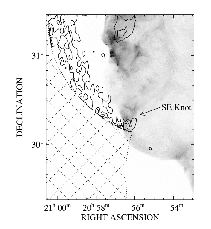
Figure 10: Contours of neutral hydrogen 21 cm emission (from Leahy, 2002) overlaid on the ROSAT HRI image. Neutral material extends up to the southeast X-ray knot but survives immediately outside, indicating that the blast wave has not fully progressed (in all projections) far beyond the X-ray knot. Farther north, H I emission is offset east of the current blast wave location, which the X-rays indicate. Contour levels are $N_{HI}=2.0$, 2.3, 2.7, and 3.0 $\times 10^{20}{\rm\,cm^{-2}}$, in the $2.64$-km-s^-1-wide band centered on $v_{LSR}=3.2{\rm\,km\,s^{-1}}$. Only warm, not cold, neutral material produces the 21 cm emission, so these contours are lower limits on the total hydrogen column density. The angular resolution of the 21 cm observations is $2\arcmin$ (E-W)$\times 4\arcmin$ (N-S), and they do not cover the area marked with dotted lines.

Observations at 21 cm (Leahy, 2002) show the distribution of warm atomic hydrogen near the southeast knot and also indicate that shocks have passed just beyond the X-ray knot. On large (degree) scales, the neutral hydrogen is distributed broadly around the outside of the SNR. At the southeast knot, H I is adjacent to the bright X-ray emission, but does not overlap it (Figure 10). This morphology suggests that a portion of the projected blast wave has just passed the X-ray knot, and the complete three-dimensional extent of the blast wave is not located far outside the X-ray knot. Farther north, the atomic hydrogen is offset to the east of the SNR blast wave, which the X-rays mark. This separation indicates that the neutral surrounding medium existed prior to the supernova, and it is not a shell of ambient material the SNR swept up. While the distance to the atomic material is uncertain, the radio emission observed in this velocity range over the whole Cygnus Loop is strongly correlated with optical and X-ray features that are characteristic of interactions of the blast wave with interstellar clouds, which indicates that this observed neutral medium and the SNR are genuinely related (Leahy, 2002).

The connection with the surrounding atomic material suggests that the X-ray- and optically-bright areas are the tip of the much larger southeast cloud. The cloud, detectable in H I, may also have a substantial cold or molecular component. We estimate the lower limit on the atomic density very roughly. Over $1^{\circ}$ scales, $N_{HI}\approx 2\times 10^{20}{\rm\,cm^{-2}}$. For a line of sight depth of $1^{\circ}$, we find $n_{HI}\approx 8{\rm\,cm^{-3}}$.

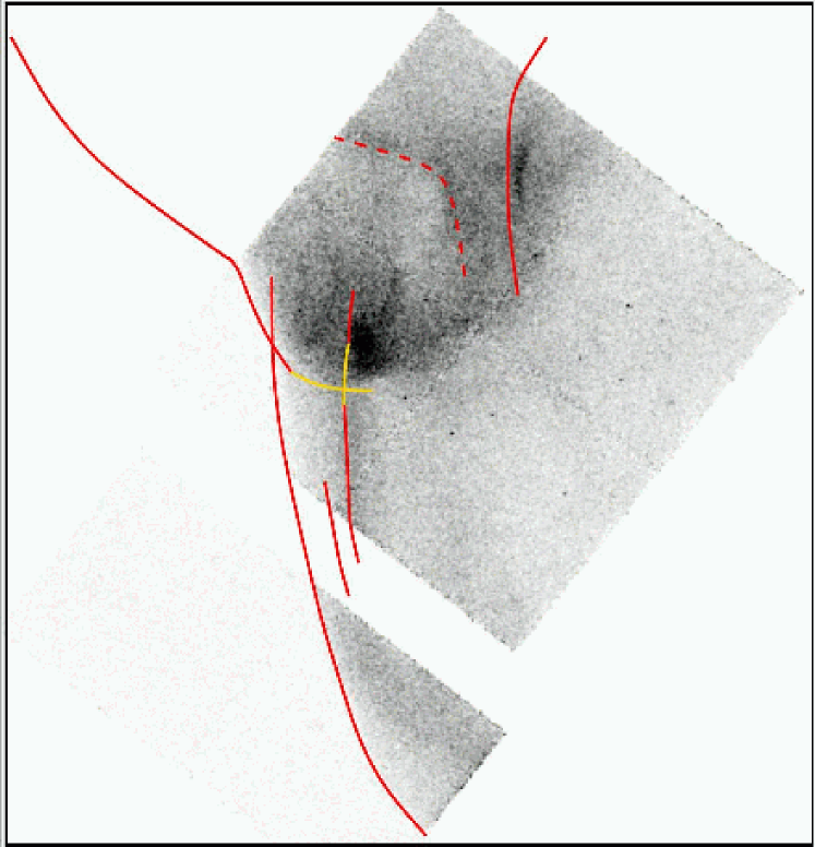
Figure 11: Projected shock front locations on the total-band image, scaled linearly from 0 (white) to $5\times 10^{-7}{\rm\,photons\,cm^{-2}\,arcsec^{-2}}$ (black). Portions of the projected shock front that are observed as Balmer filaments are drawn with solid red lines. The dominant high-temperature component measured in region C provides evidence for the shock front that interacts with the optical cloud; we identify the extended shock front (dashed red line) based on the similar total-band and color images. Overlapping projections of multiple shocks account for the brightest—yet single-temperature—area, indicating that the observed shock fronts continue into the projected interior of the SNR, marked in yellow.

The H$\alpha$ image and Chandra spectroscopy together show the location of many shock front projections. We illustrate these schematically in Figure 11. The easternmost Balmer filaments are long, arising where the blast wave is relatively undisturbed over large distances. The absolute projected edge is significantly indented relative to the near-spherical boundary of the Cygnus Loop, so a large obstacle that extends several parsecs along the line of sight impedes the blast wave. The filaments in the projected interior of the SNR are shorter and produced near smaller-scale inhomogeneities, which do not preserve a tangent view through the blast wave over large distances.

The Balmer filament near the cloud interaction of region B is offset forward (east) of the X-ray enhancement. The X-rays are due in part to the shock reflected at region C, which moves west. No Balmer filament is associated with the cloud shock of region C. The X-ray image illustrates that this shock front is extremely curved. Maintaining a large line of sight through the edge of the blast wave while it is strongly deflected around an obstacle is unlikely.

6 Conclusions

These Chandra observations of the southeast knot of the Cygnus Loop reveal details of the encounter between the supernova blast wave and a large interstellar cloud. Most of the X-ray flux arises in the interaction, with the increased density of the cloud material and reflected shocks that further compress and heat previously-shocked gas. The diffuse interior, through which the undisturbed blast wave passed, exhibits significant higher-energy emission, but having lower density, it provides less of the total flux within the field of view.

On this small scale, as throughout this SNR as a whole, the environment determines the X-ray appearance of the Cygnus Loop. The complicated morphology is fundamentally a consequence of geometry, with significant multiple projections along the line of sight. Overall, the X-ray spectra are simple and generally indicate collisional equilibrium in the post-shock regions, even when the time elapsed since the passage of the blast wave is short. Only two regions show strong evidence for non-equilibrium ionization, and electron-ion temperature equilibration behind the shock front is rapid. Optical and radio data further support interpretation of the observed spectral variations in terms of extrinsic properties of the environment. Thus, in accounting for the complex appearance of the southeastern Cygnus Loop, we do not find evidence for complex shock physics, such as fluid instabilities, or significant intrinsic variations in the evolution of the blast wave. Higher resolution spectroscopy at similar spatial resolution could yet reveal such complex physics, but these data clearly show significant spectral variations on small spatial scales, which we attribute to the SNR’s environment.

Table 1: Single-Temperature Spectral Models

Region	$N_{H}$	$kT$	$A$	$Z_{O}/Z_{\sun}$	Counts	$\chi^{2}$/dof
A	$1.0\pm 0.3$	$0.168\pm 0.003$	$6.1^{+1.2}_{-1.0}$	$0.35^{+0.05}_{-0.04}$	$5621$	$78/74$
B	$1.6\pm 0.3$	$0.175\pm 0.005$	$2.9^{+0.8}_{-0.6}$	$0.41^{+0.08}_{-0.07}$	$2660$	$106/68$
C	$0.9\pm 0.3$	$0.191\pm 0.005$	$1.8\pm 0.4$	$0.51^{+0.08}_{-0.07}$	$3736$	$98/72$
D	$0.8^{+0.3}_{-0.3:}$	$0.188\pm 0.005$	$1.7\pm 0.4$	$0.36^{+0.06}_{-0.05}$	$3059$	$102/69$
E	$1.2^{+0.5}_{-0.4}$	$0.169^{+0.005}_{-0.006}$	$2.0^{+0.8}_{-0.5}$	$0.45^{+0.13}_{-0.09}$	$2029$	$56/55$
F	$0.8^{+1.0}_{-0.3:}$	$0.149^{+0.008}_{-0.015}$	$1.1^{+1.4}_{-0.3}$	$0.37^{+0.18}_{-0.09}$	$693$	$37/22$
G	$2.5\pm 0.2$	$0.182^{+0.003}_{-0.004}$	$6.8^{+1.2}_{-1.0}$	$0.51^{+0.06}_{-0.05}$	$4981$	$173/86$
H	$2.3^{+0.3}_{-0.2}$	$0.189\pm 0.004$	$5.7^{+1.1}_{-0.9}$	$0.57^{+0.07}_{-0.06}$	$5410$	$188/92$
I	$1.8\pm 0.3$	$0.178^{+0.003}_{-0.004}$	$5.2^{+1.1}_{-0.8}$	$0.43^{+0.07}_{-0.06}$	$4935$	$188/88$
J	$0.5^{+0.6}_{-0.0:}$	$0.164^{+0.004}_{-0.007}$	$1.8^{+0.9}_{-0.1}$	$0.32^{+0.08}_{-0.05}$	$2128$	$69/51$
K	$1.2\pm 0.4$	$0.165^{+0.004}_{-0.005}$	$3.8^{+1.1}_{-0.8}$	$0.38^{+0.09}_{-0.07}$	$3095$	$62/69$
L1	$1.4^{+2.6}_{-0.9:}$	$0.12\pm 0.03$	$1.4^{+20}_{-1.4:}$	$0.38^{+0.98}_{-0.23}$	$294$	$10/9$
L2	$0.5^{+4.0}_{-0.0:}$	$0.145^{+0.007}_{-0.06}$	$1.0^{+140}_{-0.1}$	$0.31^{+0.09}_{-0.08}$	$653$	$27/20$
L3	$0.5^{+0.8}_{-0.0:}$	$0.151^{+0.005}_{-0.01}$	$1.4^{+1.2}_{-0.1}$	$0.29^{+0.07}_{-0.05}$	$1080$	$38/34$
L4	$0.8^{+0.6}_{-0.3:}$	$0.165^{+0.006}_{-0.008}$	$1.6^{+0.9}_{-0.4}$	$0.46^{+0.15}_{-0.11}$	$1724$	$72/48$

Note. — Parameters and errors constrained by hard limits are marked with a colon.

Table 2: Two-Temperature Spectral Models

Region	$N_{H}$	$kT_{1}$	$A_{1}$	$Z_{O}/Z_{\sun}$	$kT_{2}$	$A_{2}$	Counts	$\chi^{2}$/dof
G	$1.8^{+0.3}_{-0.5}$	$0.180^{+0.006}_{-0.004}$	$4.4^{+1.1}_{-1.4}$	$0.48^{+0.06}_{-0.05}$	$0.55^{+0.05}_{-0.07}$	$8.1^{+2.0}_{-1.8}$	$4981$	$130/84$
H	$0.5^{+0.6}_{-0.0:}$	$0.202^{+0.006}_{-0.013}$	$1.6^{+0.6}_{-0.2}$	$0.53^{+0.09}_{-0.07}$	$0.69^{+0.08}_{-0.06}$	$6.9^{+1.5}_{-1.7}$	$5410$	$152/90$
I	$0.8^{+0.4}_{-0.3:}$	$0.175^{+0.006}_{-0.005}$	$2.8^{+1.2}_{-0.5}$	$0.40^{+0.07}_{-0.06}$	$0.54^{+0.06}_{-0.07}$	$7.5^{+1.9}_{-1.4}$	$4935$	$120/86$

Table 3: Plane-Parallel Shock Models

Region	$N_{H}$	$kT$	$A$	$Z_{O}/Z_{\sun}$	$\tau$	Counts	$\chi^{2}$/dof
A	$1.9^{+0.5}_{-0.9}$	$0.174^{+0.007}_{-0.009}$	$7.2^{+1.7}_{-1.3}$	$0.48\pm 0.12$	$0.84^{+5}_{-0.4}$	$5621$	$74/73$
C	$1.7^{+0.7}_{-0.8}$	$0.198^{+0.02}_{-0.009}$	$2.1^{+0.7}_{-0.5}$	$0.67\pm 0.2$	$1.0^{+5}_{-0.6}$	$3736$	$94/71$
F	$2.5^{+3.1}_{-1.0}$	$0.15^{+0.03}_{-0.05}$	$2.5^{+180}_{-1.5}$	$0.56\pm 0.2$	$0.24^{+0.6}_{-0.2}$	$693$	$28/21$
J	$0.5^{+1.5}_{-0.0:}$	$0.32^{+0.06}_{-0.2}$	$0.3^{+2.2}_{-0.1}$	$0.46^{+0.1}_{-0.07}$	$0.021^{+0.34}_{-0.005}$	$2128$	$63/50$

Note. — Parameters and errors constrained by hard limits are marked with a colon.

Table 4: Combined Edge Region Spectral Model

Region	$N_{H}$	$kT$	$A$	$Z_{O}/Z_{\sun}$	Counts	$\chi^{2}$/dof
	$0.5^{+0.4}_{-0.0:}$			$0.35^{+0.07}_{-0.04}$		$153/117$
L1		$0.135^{+0.011}_{-0.013}$	$0.5^{+0.4}_{-0.2}$		$294$
L2		$0.146^{+0.006}_{-0.009}$	$0.9^{+0.5}_{-0.2}$		$653$
L3		$0.153^{+0.005}_{-0.008}$	$1.3^{+0.6}_{-0.2}$		$1080$
L4		$0.165^{+0.003}_{-0.004}$	$1.6^{+0.6}_{-0.2}$		$1724$

Note. — Parameters and errors constrained by hard limits are marked with a colon.

Figure 5: ACIS spectrum of region A (crosses) with the equilibrium model (histogram). The thermal plasma is at temperature $0.17$ keV, absorbed by $N_{H}=1.0\times 10^{21}{\rm\,cm^{-2}}$.

Figure 6: ACIS spectrum of region H (crosses) with the best-fitting model (histogram), on the same scale as Figure 5. The model includes two thermal equilibrium plasmas, at temperatures 0.16 and 0.57 keV, absorbed by $N_{H}=2.1\times 10^{21}{\rm\,cm^{-2}}$.

Figure 7: ACIS spectrum of region F (crosses) with the best-fitting model (histogram). The non-equilibrium ionization plane-parallel shock model has equilibrium temperature $kT=0.15$ keV, ionization timescale $\tau=2.4\times 10^{12}{\rm\,cm^{-3}\,s}$, and is absorbed by $N_{H}=2.5\times 10^{21}{\rm\,cm^{-2}}$.

References

- Anders & Grevesse (1989) Anders, E., & Grevesse, N. 1989, Geochim. Cosmochim. Acta, 53, 197
- André et al. (2003) André, M. K., et al. 2003, ApJ, 591, 1000
- Arnaud (1996) Arnaud, K. A. 1996, in ASP Conf. Ser. 101, Astronomical Data Analysis Software and Systems V, ed. G. Jacoby & J. Barnes (San Francisco:ASP), 17
- Arnaud & Rothenflug (1985) Arnaud, M., & Rothenflug, M. 1985, A&AS, 60, 425
- Blair et al. (1999) Blair, W. P., Sankrit, R., Raymond, J. C., & Long, K. S. 1999, AJ, 118, 942
- Borkowski, Sarazin, & Blondin (1994) Borkowski, K. J., Sarazin, C. L., & Blondin, J. M. 1994, ApJ, 429, 710
- Cargill & Papadopoulos (1988) Cargill, P. J., & Papadopoulos, K. 1988, ApJ, 329, L29
- Chevalier & Raymond (1978) Chevalier, R. A., & Raymond, J. C. 1978, ApJ, 225, L27
- Fesen et al. (1992) Fesen, R. A., Kwitter, K. B., & Downes, R. A. 1992, AJ, 104, 719
- Ghavamian et al. (2001) Ghavamian, P., Raymond, J., Smith, R. C., & Hartigan, P. 2001, ApJ, 547, 995
- Gorenstein, Tucker, & Harnden (1974) Gorenstein, P., Harnden, F. R., Jr., & Tucker, W. H. 1974, ApJ, 192, 661
- Graham et al. (1995) Graham, J. R., Levenson, N. A., Hester, J. J., Raymond, J. C., & Petre, R. 1995, ApJ, 444, 787
- Hamilton, Chevalier, & Sarazin (1983) Hamilton, A. J. S., Chevalier, R. A., & Sarazin, C. L. 1983, ApJS, 51, 115
- Hester & Cox (1986) Hester, J. J., & Cox, D. P. 1986, ApJ, 300, 675
- Hester et al. (1994) Hester, J. J., Raymond, J. C., & Blair, W. P. 1994, ApJ, 420, 721
- Klein, McKee, & Colella (1994) Klein, R. I., McKee, C. F., & Colella, P. 1994, ApJ, 420, 213
- Laming et al. (1996) Laming, J. M., Raymond, J. C., McLaughlin, B. M., & Blair, W. P. 1996, ApJ, 472, 267
- Leahy (2002) Leahy, D. A. 2002, AJ, 123, 2689
- Levenson et al. (1997) Levenson, N. A., et al. 1997, ApJ, 484, 304
- Levenson & Graham (2001) Levenson, N. A., & Graham, J. R. 2001, ApJ, 559, 948
- Levenson et al. (1998) Levenson, N. A., Graham, J. R., Keller, L. D., & Richter, M. J. 1998, ApJS, 118, 541
- Levenson et al. (2002) Levenson, N. A., Graham, J. R., & Walters, J. L. 2002, ApJ, 576, 798
- Liedahl (1999) Liedahl, D. A. 1999, in Lecture Notes in Physics 520, X-ray Spectroscopy in Astrophysics, ed. J. van Paradijs & J. A. M. Bleeker (Heidelberg:Springer), 189
- Liedahl et al. (1995) Liedahl, D. A., Osterheld, A. L., & Goldstein, W. H. 1995, ApJ, 438, L115
- Mazzotta et al. (1998) Mazzotta, P., Mazzitelli, G., Colafrancesco, S., & Vittorio, N. 1998, A&AS, 133, 403
- Mewe, Gronenschild, & van den Oord (1985) Mewe, R., Gronenschild, E. H. B. M., & van den Oord, G. H. J. 1985, A&AS, 62, 197
- Mewe, Lemen, & van den Oord (1986) Mewe, R., Lemen, J. R., & van den Oord, G. H. J. 1986, A&AS, 65, 511
- Meyer et al. (1998) Meyer, D. M., Jura, M., & Cardelli, J. A. 1998, ApJ, 493, 222
- Rakowski, Ghavamian, & Hughes (2003) Rakowski, C. E., Ghavamian, P., & Hughes, J. P. 2003, ApJ, 590, 846
- Raymond, Blair, & Long (1995) Raymond, J. C., Blair, W. P., & Long, K. S. 1995, ApJ, 454, L31
- Raymond et al. (2003) Raymond, J. C., Ghavamian, P., Sankrit, R., Blair, W. P., & Curiel, S. 2003, ApJ, 584, 770
- Shull & van Steenberg (1982) Shull, J. M., & van Steenberg, M. 1982, ApJS, 48, 95
- Spitzer (1962) Spitzer, L. 1962, Physics of Fully Ionized Gases, 2nd ed. (New York:Interscience)
- Spitzer (1940) Spitzer, L., Jr. 1940, MNRAS, 100, 396
- Townsley et al. (2000) Townsley, L. K.. Broos, P. S., Garmire, G. P., & Nousek, J. A. 2000, ApJ, 534, L139
- Welty et al. (1999) Welty, D. E., Hobbs, L. M., Lauroesch, J. T., Morton, D. C., Spitzer, L., & York, D. G. 1999, ApJS, 124, 465