Simulations of the relativistic parsec-scale jet in 3C 273

Abstract

We present a hydrodynamical 3D simulation of the relativistic jet in 3C273, in comparison to previous linear perturbation analysis of Kelvin-Helmholtz instability developing in the jet. Our aim is to assess advantages and limitations of both analytical and numerical approaches and to identify spatial and temporal scales on which the linear regime of Kelvin-Helmholtz instability can be applied in studies of morphology and kinematics of parsec-scale jets.

1 Introduction

3C 273 is the brightest quasar known. Due to its relative closeness ($z=0.158$), it has become a prime target for studies in all spectral bands aimed at understanding the AGN phenomenon (Courvoisier, 1998). Radio emission from the jet in 3C 273 has been observed on parsec scales using VLBI (Pearson et al., 1981; Krichbaum et al., 2000; Abraham et al., 1996; Lobanov & Zensus, 2001). Lobanov & Zensus (2001,  LZ01 hereafter) interpreted structures observed in the parsec-scale jet of 3C 273 as a double helix and applied linear analysis of Kelvin-Helmholtz instability (e.g., Hardee 2000) to infer the basic parameters of the flow. Asada et al. (2002) suggest that a helical magnetic field could generate similar patterns in the jet. LZ01 obtain a bulk Lorentz factor $W=2.1$, well below those measured for superluminal components ($W=5-10$, Abraham et al. 1996), but suggest that instabilities develop in the slower underlying flow, interpreting those fast components as shock waves inside the jet. This result, if confirmed, would make the combination of observations and linear stability theory a powerful tool for probing the physical conditions in relativistic jets. We aim here to compare the results of the analytical modelling to the structures generated in a numerical simulation of a steady jet, with the initial conditions of the underlying flow given in LZ01. The jet is perturbed with several helical and elliptical modes, which correspond to the modes identified by LZ01. Previous works by Perucho et al. (2004a; 2004b) have shown that numerical simulations can be used to study the transition from the linear to the non-linear regime, and we will apply this approach to investigate whether the results obtained from the numerical and linear methods can be reconciled.

2 Numerical simulation

2.1 Initial setup

We start with a steady jet, which has a Lorentz factor $W=2.1$, density contrast with the external medium $\eta=0.023$, sound speed $c_{s,j}=0.53\,c$ in the jet and $c_{s,a}=0.08\,c$ in the external medium and perfect gas equation of state (with adiabatic exponent $\gamma=4/3$). Assuming an angle to the line of sight $\theta=15^{\circ}$ and redshift $z=0.158$ ($1\,\rm{mas}=2.43\,\rm{pc}$), the observed jet is $169\,h^{-1}\rm{pc}$ long (with the modified Hubble constant $H_{0}=70\times h\,\rm{km}\,\rm{s}^{-1}\rm{Mpc}^{-1}$. Considering the jet radius given in LZ01 ($0.8\,\rm{pc}$), the numerical grid is $211\,R_{j}$ (axial) times $8\,R_{j}$ (transversal), i.e., $169\,\rm{pc}\times 6.4\,\rm{pc}$.

Resolution is $16\,{\rm cells}/R_{j}$ in the transversal direction and $4\,{\rm cells}/R_{j}$ in the direction of the flow. A shear layer of $2\,R_{j}$ width is included in the initial rest mass density and axial velocity profiles to keep numerical stability of the initial jet. Elliptical and helical modes are induced at the inlet.

$\lambda^{obs}$	Mode	$\lambda^{theor}$	$\lambda^{sim}$	$\lambda^{sim}_{v_{w}=0.23\,c}$	$\lambda^{sim}_{v_{w}=0.38\,c}$	$\lambda^{sim}_{v_{w}=0.88\,c}$
(mas)		($R_{j}$)	($R_{j}$)	(mas)	(mas)	(mas)
2	$H_{b2}$	18.7	4	0.44	0.54	2.27
4	$E_{b1},H_{b1}$	37.4	25	2.7	3.37	14.3
12	$E_{s}$	21.2a	50	5.5	6.7	28.5

Table 1: First two columns give identified wavelengths and modes in LZ01 ($H$ stands for helical, $E$ for elliptical, $s$ for surface mode and $b1$ and $b2$ for first and second body modes, respectively), third column gives the intrinsic wavelengths (see text), in the fourth column we have written observed wavelengths in the simulation, and the last three columns give the fourth column wavelengths as observed depending on the wave speed. ^a Computed assuming it propagates with the flow speed.

Frequencies of the excited modes are computed from the observed wavelengths, $\lambda^{obs}$, corrected for projection effects, relativistic motion and propagation speed of the instability, $v_{w}$. This yields $\omega=2\,\pi\,v_{w}/\lambda^{theor}$, with

$$\lambda^{theor}=\frac{\lambda^{obs}(1-v_{w}/c\,\cos\theta)}{\sin\theta}\,.$$ (1)

We use $v_{w}=0.23\,c$ for all body modes identified in LZ01 (see Table 1). The surface modes are assumed to move with a speed close to that of the jet (e.g., Hardee 2000). The $18\,\rm{mas}$ mode in LZ01, which is not identified with any Kelvin-Helmholtz mode, was not included in this simulation. Table 1 lists the modes which have been excited in the simulation. The simulation lasted for a time $1097\,R_{j}/c$ (i.e., $\simeq 2852\,\rm{yrs}$), and it used $\simeq 11$ Gb RAM Memory and $8$ processors during around $30$ days in a SGI Altix 3000 computer.

2.2 Discussion

The simulation run can be divided in two different parts. In the first part, the instability grows linearly. In the second part, disruption occurs and it dominates further evolution of the flow. In Figs. 1 and 2, we display several transversal cuts and axial cuts at two different times of the simulation, respectively. The transverse cuts illustrate mode competition showing that different modes dominate at different positions and times in the jet. The longitudinal structures presented in Figs. 2 and 3 indicate that the linear phase of the instability growth is dominated by the short helical mode ($\simeq 4\,R_{j}$) modulated by the longer helical (antisymmetric, $\simeq 20\,R_{j}$) and elliptical (symmetric, $\simeq 50\,R_{j}$) modes.

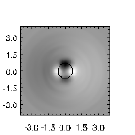
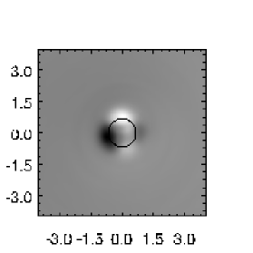
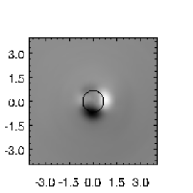
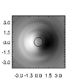
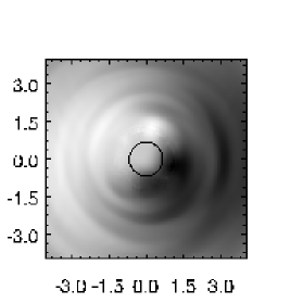
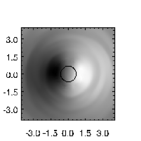
Figure 1: Map of pressure perturbation transversal cuts in arbitrary units, values increasing from dark to lighter colors. Solid line indicates $v_{z}=0.8\,c$ contour. Three left panels: Cuts at $35\,R_{j}$, $t=70,\,140,\,200\,R_{j}/c$ where elliptical mode rotation is apparent. Three right panels: Cuts at $105\,R_{j}$, $t=210,\,220,\,240\,R_{j}/c$ where helical mode rotation is apparent.

The linear growth of instability ends up with the disruption of the jet caused by one of the longest helical modes ($\simeq 20\,R_{j}$), at time $t=350\,R_{j}/c$. After disruption, evolution of the jet is totally influenced by this mode, and it induces perturbations that propagate slowly backwards as a backflow in the ambient medium. The disruption point moves outwards due to the constant injection of momentum at the inlet and the change of conditions around the jet, which seem to make it more stable. This point moves from $160\,\rm{R_{j}}$ to $180\,\rm{R_{j}}$ by the end of the simulation (see Fig. 2).

To check the consistency of the results obtained for the linear regime of the simulation with observed structures, we need to measure the propagation speeds of the perturbations. The time step between subsequent frames is too large to measure these speeds directly from the simulation data, and we use pressure perturbations profiles for this purpose. From pressure perturbation plots (see Fig. 3), we estimate the velocity of propagation of the fastest modes by measuring the position of the perturbation front in each frame. In this way, we find perturbations which travel with a velocity close to that of the flow ($v_{w}\simeq 0.88\,c$ as an upper limit). We can also derive the wave speed of the disruptive mode following the motion of the large amplitude wave (see Fig. 2) from frame to frame, and we find $v_{w}\simeq 0.38\,\rm{c}$. We can associate the former, faster perturbation, with the longer wavelength and longer exponential growth length elliptical surface mode (see Fig. 3), and the latter with a shorter wavelength and shorter exponential growth length body mode (see Hardee 2000). Both measured speeds are different to that given by LZ01 ($0.23\,c$). This difference may be caused by an accumulation of errors in different assumptions, or even by the excitation of a slightly different (implying different velocity). The observer frame wavelengths calculated for different values of the propagation speed are given in Table 1.

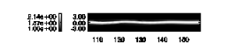
Figure 2: Map of Lorentz factor distribution of a portion of the jet at a time before disruption, where a large amplitude wave is apparent (top panel, $t=320\ R_{j}/c$) and at the last frame (bottom panel, $t=1097\,R_{j}/c$). Coordinates are in jet radii. Note that the vertical scale size is increased by a factor of 4 for the sake of clarity.

3 Conclusions

We have shown that the structures found in a jet with the physical properties of the underlying flow given in LZ01, and perturbed with elliptical and helical modes, are of the same order in size as those observed, if relativistic propagation effects of the waves are taken into account. Although there is a difference between wave speeds found in this work and that derived from linear analysis and we do not find a unique combination of parameters which explain observed structures, we show in Table 1 that similar wavelengths to those observed are found for given combinations of measured wavelengths in the simulation and wave speeds.

Figure 3: Longitudinal cut of pressure perturbation at $R_{j}/2$ in symmetric positions with respect to the jet axis at $t=250\,R_{j}/c$. Helical (antisymmetric) structures of $4$ and $25\,R_{j}$ and an elliptic (symmetric) one of $50\,R_{j}$ are apparent.

Our simulations do not address the question of long term stability of the jet. The simulated jet is disrupted at distances of $\sim 170\,h^{-1}\,\rm{pc}$, which is much shorter than the observed $\sim 60\,h^{-1}\,\rm{kpc}$ extent of the jet in 3C 273. A combination of five different factors may be responsible for this discrepancy. 1) Magnetic fields have not been taken into account neither in the linear analysis, nor in the numerical simulation, but they may be dynamically important at parsec scales. 2) We only simulate the underlying flow, without taking into account the superluminal components. 3) Initial amplitudes of perturbations cannot be constrained accurately. 4) Inaccuracies in the approximations used in the linear analysis can lead to differences in physical parameters derived. 5) Differential rotation of the jet, shear layer thickness, and a decreasing density of the external medium could affect the wavelengths and speeds of the instability modes. The combined effect of these factors could well change the stability properties of the jet.