Triaxial haloes, intrinsic alignments and the dark matter power spectrum

Abstract

We develop the halo model of large-scale structure to include triaxial dark matter haloes and their intrinsic alignments. As a direct application we derive general expressions for the two-point correlation function and the power spectrum. We then focus on the power spectrum and numerically solve the general expressions for two different models of the triaxial profiles. The first is a toy-model that allows us to isolate the dependence of clustering on halo shape alone and the second is the more realistic profile model of Jing & Suto (2002). In both cases, we find that the effect of triaxiality is manifest as a suppression of power at the level of $\sim 5\%$ on scales $k\sim 1-10\,h{\rm Mpc}^{-1}$, which in real space corresponds to the virial radii of clusters. When considered by mass, we find that for the first model the effects are again apparent as a suppresion of power and that they are more significant for the high mass haloes. For the Jing & Suto model, we find a suppression of power on large scales followed by a sharp amplification on small scales at the level of $\sim 10-15\%$. Interstingly, when averaged over the entire mass function this amplification effect is surpressed. We also find for the 1-Halo term on scales $k<10\,h{\rm Mpc}^{-1}$, that the power is dominated by ellipsoidal haloes with semi-minor to semi-major axis ratios $a/c<0.7$.

One of the important features of our formalism is that it allows for the self-consistent inclusion of the intrinsic alignments of haloes. The alignments are specified through the correlation function of halo seeds. We develop a useful toy model for this and then make estimates of the alignment contribution to the power spectrum. Further, through consideration of the (artificial) case where all haloes are perfectly aligned, we calculate the maximum possible contribution to the clustering. We find the hard limit of $<10\%$. Subject to further scrutiny, the proposed toy-model may serve as a means for linking the actual observed intrinsic alignments of galaxies to physical quantities of interest.

1 Introduction

It is well known that the correlation functions for the dark matter contain a wealth of information about the cosmological model, the physics of the dark matter and the relative mix of baryons, photons and neutrinos (see Bond & Efstatiou, 1984; Seljak & Zaldarriaga, 1996; Eisenstein & Hu, 1998). However, it is less well known that they also contain information concerning the shapes of the structures that form. Under the assumption that the initial density field is Gaussian random, then during the linear stages of gravitational collapse all of the correlation functions, except for the 2-pt function, are zero and the fluctuations are effectively shapeless. However, under continued gravitational collapse, asymmetries develop and are amplified. For the hierarchical Cold Dark Matter (CDM) models this results in halo formation and then the emergence of the ‘cosmic web’ (Bond & Myers, 1996). Subsequently, all of the higher order correlation functions are non-zero and must now contain information about the morphological structure of the density field.

Recent attempts to model the 2-pt correlation function have shown that qualitatively this can be matched with no further assumption than: that the haloes that form are spherical with some particular density profile (Navarro, Frenk & White, 1997, hereafter NFW); that the large-scale over-densities are ellipsoidal (Sheth, Mo & Tormen, 2000); and that halo formation is preferential in the regions of large-scale over-density (Sheth & Tormen, 1999, hereafter ST). However, when this approach is used to model the 3-pt correlation function, significant discrepancies are found (Scoccimarro et al., 2001). Currently, the root of these discrepancies is believed to be simply due to the triaxiality of dark matter haloes. However, this has yet to be explicitly shown.

Furthermore, whilst the 2-pt statistics can be qualitatively reproduced with simplified models, it still remains to be seen whether these approaches can be made to precisely match results in general (Smith et al., 2003; Huffenberger & Seljak, 2003). With current galaxy redshift surveys, such as the 2-degree Field Redshift Survey (Colless et al., 2001) and the Sloan Digital Sky Survey (Strauss et al., 2002), being sufficiently large enough to produce hi-fidelity measurements of the 2-pt (Percival et al., 2001; Hawkins et al., 2003; Zehavi et al., 2002; Tegmark et al., 2004) and 3-pt galaxy clustering statistics (Jing & Börner, 2004; Kayo et al., 2004), and with planned cosmic weak shear surveys expected to be capable of measuring the projected 2-pt and 3-pt matter clustering statistics to similar levels of accuracy (Aldering et al., 2004), resolving these issues becomes important.

In this and subsequent work, we will explore these questions in detail. Our first aim, in this paper, is to develop a self-consistent analytic model that allows us to make predictions for the nonlinear dark matter clustering signal, given information about the cosmological model and now, additionally, the shapes of dark matter haloes and also their intrinsic alignments. A second aim will be to provide, as an application of the model, predictions for the 2-pt clustering statistics. We achieve these goals by developing the halo-model of large-scale structure (Seljak 2000; Peacock & Smith 2000; Ma & Fry 2000; and for a review see Cooray & Sheth 2003).

An important by-product of this work is that the inclusion of halo shapes allows one to study the intrinsic alignments of dark matter haloes alone. This is achieved through the inclusion of the correlation function of halo axis direction vectors, and we develop a toy-model to explore the effects of halo alignment on the power spectrum.

The outline of this paper is as follows. In Section 2.1, we define some useful theoretical notions. In Section 2.2 we present the triaxial halo model formalism and provide a derivation for the 2-pt correlation function. In Sections 2.3–2.5 we derive the power spectrum. In Section 3, we flesh-out the necessary details for performing calculations. In particular we consider two interesting models for the density profile of triaxial haloes: the first is a toy model that we have developed to explore how halo shape alone affects the clustering statistics; the second is the more realistic model of Jing & Suto (2002, hereafter JS02). Here, we also develop our toy model for the intrinsic alignments correlation function. In Section 4, we present our results, and finally in Section 5 we discuss our findings and present the conclusions.

Throughout, we have assumed that the cosmological model is the concordance model (Wang et al., 2000) and that the linear power spectrum is given by Efstathiou, Bond & White (1992) with normalization $\sigma_{8}=0.9$ and shape parameter $\Gamma=0.21$.

2 Theory

2.1 Basic definitions

In what follows, we will seek to compute the lowest order clustering statistic of interest, that is the power spectrum of mass fluctuations, $P({\bf k})$. This is defined by

$$\langle\delta({\bf k})\,\delta({\bf k}^{\prime})\rangle=(2\pi)^{3}P({\bf k})\,\delta^{D}({\bf k}-{\bf k}^{\prime})\ ,\$$ (1)

where $\delta({\bf k})$ is the Fourier transform of the density fluctuation field $\delta({\bf x})=\rho({\bf x})/\bar{\rho}-1$ and $\bar{\rho}$ is the background density; angle brackets denote the ensemble average and $\delta^{D}$ is the Dirac delta function. The Power Spectrum is itself the Fourier transform of the real space 2-pt correlation function $\xi({\bf r})$, which can be similarly defined

$$\xi({\bf r})=\langle\delta({\bf x})\,\delta({\bf x}+{\bf r})\rangle\ .$$ (2)

In the above definitions we have considered general anisotropic density fields. However, in cosmological applications it is usual to assume statistical isotropy and homogeneity of the Universe, hence these quantities become functions of scalar arguments only. In the work that follows, we will not make the above assumptions, since we are dealing with anisotropic dark matter haloes, but will show that for the power spectrum the scalar arguments that we desire will naturally emerge from our formalism.

It will also prove useful to define some basic relations for the triaxial haloes (see Chandrasekhar, 1969, for a full treatise). We start by considering an heterogeneous triaxial ellipsoid that has semi-axis lengths $a$, $b$ and $c$, where $a\leq b\leq c$, and orthogonal principle axis vectors $\hat{\bf{e}}_{a}$, $\hat{\bf{e}}_{b}$ and $\hat{\bf{e}}_{c}$. We define the triaxial coordinate system $(R,\Theta,\Phi)$ with respect to the principle axes of the halo, where $\hat{\bf{e}}_{c}$ is taken to be in the $z$-direction. The radial parameter $R$ traces out thin iso-density shells, or homoeoids, and the parameters $\Theta$ and $\Phi$ are the polar and azimuthal angles respectively. In this system the Cartesian components are

$$x=\frac{a}{c}R\cos\Phi\sin\Theta\ ;\ y=\frac{b}{c}R\sin\Phi\sin\Theta\ ;\ z=R\cos\Theta.$$ (3)

It is to be noted that the ellipsoidal angles differ from those of the spherical coordinate system. The parameter $R$ can be related to the Cartesian coordinates and axis ratios through

$$\frac{R^{2}}{c^{2}}=\frac{x^{2}}{a^{2}}+\frac{y^{2}}{b^{2}}+\frac{z^{2}}{c^{2}}\ .$$ (4)

The benefits of this choice of coordinate system are now apparent: if all the homoeoidal shells are concentric, and if we pick coordinates with the same axis ratios as the triaxial ellipsoid, then the density run of the ellipsoid can be described by a single parameter:

$$\rho({\bf r})\rightarrow\rho(R)\ .$$ (5)

Furthermore, the mass enclosed within some iso-density cut-off scale $R_{\rm cut}$, can be obtained most simply by

$$M=\int_{R_{\rm cut}({\bf r})}d^{3}\!r\rho({\bf r})=4\pi\frac{ab}{c^{2}}\int_{0}^{R_{\rm cut}}dRR^{2}\rho(R)\ ,$$ (6)

where the ellipsoidal coordinates have allowed us to circumvent the problem of evaluating complicated halo boundaries.

It is now convenient to define what we mean by a halo: any object that has a volume averaged over-density 200 times the background density is considered to be a gravitationally bound halo of dark matter. This leads directly to the following relation between the mass, radius and axis ratios:

$$M_{200}=\frac{4}{3}\pi R_{200}^{3}{\left(\frac{ab}{c^{2}}\right)}200\bar{\rho}\ .$$ (7)

The above definition was adopted in order to be consistent with the mass-function of ST, which we utilize in what follows.

2.2 The triaxial halo model

In earlier implementations of the halo-model it was assumed that all of the matter in the Universe was contained within spherical dark matter haloes with some particular density profile and some distribution of mass (Seljak, 2000; Peacock & Smith, 2000; Ma & Fry, 2000). We now re-develop the halo model formalism making the important modification that haloes are not in general spherical, but instead are more closely described by the family of triaxial ellipsoids.

To start, we characterize each halo in terms of a set of stochastic variables that describe both shape and orientation: a given halo of mass $M$ will therefore have principle axis vectors $\hat{\bf{e}}_{a}$, $\hat{\bf{e}}_{b}$ and $\hat{\bf{e}}_{c}$ with axis ratios $a/c$ and $b/c$. The density run of a particular halo is described by the function $\rho({\bf r},M,\mbox{\boldmath$\mathcal{E}$},{\bf a})\equiv M\,U({\bf r},M,\mbox{\boldmath$\mathcal{E}$},{\bf a})$, where $U$ is the mass normalized profile, and we have introduced the shorthand notation $\mbox{\boldmath$\mathcal{E}$}\equiv(\hat{\bf{e}}_{a},\hat{\bf{e}}_{b},\hat{\bf{e}}_{c})$ and ${\bf a}\equiv(a,b,c)$. The density at any point can now be expressed simply as a sum over the $N$ haloes that form the field

$$\rho({\bf r})=\sum_{i}^{N}M_{i}\,U({\bf r}-{\bf x}_{i},M_{i},\mbox{\boldmath$\mathcal{E}$}_{i},{\bf a}_{i}),$$ (8)

where ${\bf x_{i}}$ denotes the position vector of the centre of mass of the $i^{\rm th}$ halo. Following Scherrer & Bertschinger (1991), we can re-write the sum in equation (8) using the substitution

$$\sum_{i} \rightarrow \int d{\bf x}\,dM\,d\mbox{\boldmath$\mathcal{E}$}\,d{\bf a}\sum_{i}{\delta^{D}}({\bf x}-{\bf x}_{i})\,{\delta^{D}}(M-M_{i})$$ (9)

$$\times\,{\delta^{D}}(\mbox{\boldmath$\mathcal{E}$}-\mbox{\boldmath$\mathcal{E}$}_{i})\,{\delta^{D}}({\bf a}-{\bf a}_{i})\ ,$$

which allows us to consider integrals over continuous variables rather than a sum over discrete quantities. The integral over $\mathcal{E}$ in the above expression indicates an integral over all possible orientations of the halo. The orientation of the halo frame can be specified relative to a fixed Cartesian basis set through the Euler angles. These represent successive rotations of the halo frame about the $z$–axis by $\alpha$, the $y^{\prime}$–axis by $\beta$, and the $z^{\prime\prime}$–axis by $\gamma$ (see Mathews & Walker, 1970). Hence the process of averaging over all possible halo orientations can be performed by integrating over all possible Euler angles.

Lastly, to compute the ensemble averages we integrate over the joint probability density function for the $N$ haloes that form the density field, and sum over the probabilities for obtaining the $N$ haloes (see McClelland & Silk, 1977, for a similar approach):

$$\langle\cdot\cdot\cdot\rangle\equiv\sum_{j}p(N_{j}|V)\int\prod_{i=1}^{N_{j}}dM_{i}\;d^{3}x_{i}\;d{\bf a}_{i}\;d\mbox{\boldmath$\mathcal{E}$}_{i}$$

$$\hskip 14.22636pt\times p(M_{1},..,M_{N_{j}},{\bf x}_{1},..,{\bf x}_{N_{j}},{\bf a}_{1},..,{\bf a}_{N_{j}},\mbox{\boldmath$\mathcal{E}$}_{1},..,\mbox{\boldmath$\mathcal{E}$}_{N_{j}}|N_{j})\ .$$ (10)

Provided the volume of space considered is large, then $p(N|V)$ is very sharply spiked around $N=\bar{n}V\gg 1$, where $\bar{n}$ is the mean number density of haloes. We restrict our study to this case only. Also, the ensemble average of equation (8) gives the mean density of the universe, $\bar{\rho}$.

To compute the 2-point correlation function of the triaxial halo field we substitute equations (8) and (9) into (2) and compute the ensemble average according to equation (10). The result is a sum of two terms, the first accounts for the correlation between points in a single halo and the second accounts for the inter-halo correlation (hereafter the 1-Halo and 2-Halo terms):

$$\xi({\bf r})=\xi^{\rm 1H}({\bf r})+\xi^{\rm 2H}({\bf r})\ :$$ (11)

$$\xi^{\rm 1H}({\bf r})\!\!\!\! =\!\!\!\! \frac{N}{\bar{\rho}^{2}}\int dM\,d{\bf x}\,d\mbox{\boldmath$\mathcal{E}$}\,d{\bf a}\;M^{2}\,p({\bf x},M,\mbox{\boldmath$\mathcal{E}$},{\bf a})$$ (12)

$$\times\;U({\bf r}_{1}-{\bf x},M,\mbox{\boldmath$\mathcal{E}$},{\bf a})\;U({\bf r}_{2}-{\bf x},M,\mbox{\boldmath$\mathcal{E}$},{\bf a})-1\ ;$$

$$\xi^{\rm 2H}({\bf r})\!\!\!\! =\!\!\!\! \frac{N^{2}}{\bar{\rho}^{2}}\int dM_{1}\,dM_{2}\,d{\bf x}_{1}\,d{\bf x}_{2}\,d\mbox{\boldmath$\mathcal{E}$}_{1}\,d\mbox{\boldmath$\mathcal{E}$}_{2}\,d{\bf a}_{1}\,d{\bf a}_{2}\,M_{1}\,\,M_{2}\,$$ (13)

$$\times\;U({\bf r}_{1}-{\bf x}_{1},M_{1},\mbox{\boldmath$\mathcal{E}$}_{1},{\bf a}_{1})\,U({\bf r}_{2}-{\bf x}_{2},M_{2},\mbox{\boldmath$\mathcal{E}$}_{2},{\bf a}_{2})$$

$$\times\;p({\bf x}_{1},{\bf x}_{2},M_{1},M_{2},\mbox{\boldmath$\mathcal{E}$}_{1},\mbox{\boldmath$\mathcal{E}$}_{2},{\bf a}_{1},{\bf a}_{2})-1\ ,$$

where the separation vector ${\bf r}={\bf r}_{1}-{\bf r}_{2}$.

The joint probability density function in the 2-Halo term may be written:

$$p(1,2)=p(1)\,p(2)\left[1+\xi^{\rm s}(1,2)\right]\ ,$$ (14)

where we have adopted the short-hand notation $p(1)\equiv p({\bf x}_{1},M_{1},\mbox{\boldmath$\mathcal{E}$}_{1},{\bf a}_{1})$, and where $\xi^{\rm s}$ is the seed-correlation function, which describes the relationship between a particular halo’s characteristics and those of all the other haloes. In the spherical halo model this would just be the halo-bias of Mo & White (1996), however in the triaxial model the function is more complicated, with halo orientation vectors and shapes being influenced by those of neighbouring objects. We explore this in greater detail in Section 2.5.

Neglecting for the time being $\xi^{\rm s}(1,2)$, all that remains to arrive at the correlation function in the triaxial halo model is to deal with the joint probability density function for a single halo’s characteristics: $p(1)$. We assume that a halo’s orientation, position and mass are independent random variables, and that the halo axis ratios are dependent on mass only. Hence we have:

$$p({\bf x},M,\mbox{\boldmath$\mathcal{E}$},{\bf a})=\frac{1}{V}\frac{n(M)}{\bar{n}}p(\mbox{\boldmath$\mathcal{E}$})p({\bf a}|M),$$ (15)

where $n(M)$ is the halo mass function. In order to provide a uniform probability for the halo orientation on the sphere, the density function $p(\mbox{\boldmath$\mathcal{E}$})$ takes the form

$$p(\mbox{\boldmath$\mathcal{E}$})d\mbox{\boldmath$\mathcal{E}$} \equiv p(\alpha,\beta,\gamma)d\alpha\,d\beta\,d\gamma\ ,$$ (16)

$$= \frac{1}{2\pi}\frac{1}{2}\frac{1}{2\pi}\,d\alpha\,d(\cos\beta)\,d\gamma,$$

where the variables are restricted to the ranges: $0\geq\alpha\geq 2\pi$, $0\geq\beta\geq\pi$ and $0\geq\gamma\geq 2\pi$. On substituting equations (14) and (15) into (12) and (13) we find:

$$\xi^{\rm 1H}({\bf r})\!\! = \frac{1}{\bar{\rho}^{2}}\int dM\,d{\bf x}\,d\mbox{\boldmath$\mathcal{E}$}\,d{\bf a}\,M^{2}\,n(M)\,p(\mbox{\boldmath$\mathcal{E}$})\,p({\bf a}|M)$$ (17)

$$\times\,U({\bf r}_{1}-{\bf x})U({\bf r}_{2}-{\bf x})\ ;$$

$$\xi^{\rm 2H}({\bf r}) = \frac{1}{\bar{\rho}^{2}}\int dM_{1}\,dM_{2}\,d{\bf x}_{1}\,d{\bf x}_{2}\,d\mbox{\boldmath$\mathcal{E}$}_{1}\,d\mbox{\boldmath$\mathcal{E}$}_{2}\,d{\bf a}_{1}\,d{\bf a}_{2}\,M_{1}\,M_{2}\,$$ (18)

$$\times\;n(M_{1})\,n(M_{2})\,p(\mbox{\boldmath$\mathcal{E}$}_{1})\,p(\mbox{\boldmath$\mathcal{E}$}_{2})\,p({\bf a}_{1}|M_{1})\,p({\bf a}_{2}|M_{2})\,$$

$$\times\xi^{\rm s}(1,2)\,U_{1}({\bf r}_{1}-{\bf x}_{1})\,U_{2}({\bf r}_{2}-{\bf x}_{2})\ ;$$

where we have suppressed the explicit functional dependence of the density profile $U$ on all variables except the position vector and the subscripts refer to either halo one or two.

2.3 The dark matter power spectrum

The power spectrum of the triaxial halo field can be evaluated by taking the Fourier transform of expressions (17) and (18) to yield:

$$P({\bf k})=P^{\rm 1H}({\bf k})+P^{\rm 2H}({\bf k})\ ;$$ (19)

$$P^{\rm 1H}({\bf k}) = \frac{1}{\bar{\rho}^{2}}\int dM\,d\mbox{\boldmath$\mathcal{E}$}\,d{\bf a}\;M^{2}n(M)\,p(\mbox{\boldmath$\mathcal{E}$})\,p({\bf a}|M)$$ (20)

$$\times\tilde{U}({\bf k})\,\tilde{U}^{*}({\bf k})\ ;$$

$$P^{\rm 2H}({\bf k}) = \frac{1}{\bar{\rho}^{2}}\int dM_{1}\,dM_{2}\,d\mbox{\boldmath$\mathcal{E}$}_{1}\,d\mbox{\boldmath$\mathcal{E}$}_{2}\,d{\bf a}_{1}\,d{\bf a}_{2}\,M_{1}\,M_{2}\,$$ (21)

$$\times\;n(M_{1})\,n(M_{2})\,p(\mbox{\boldmath$\mathcal{E}$}_{1})\,p(\mbox{\boldmath$\mathcal{E}$}_{2})\,p({\bf a}_{1}|M_{1})\,p({\bf a}_{2}|M_{2})\,$$

$$\times\;P^{\rm s}(1,2)\,\tilde{U}({\bf k})\,\tilde{U}^{*}({\bf k}),$$

where $\tilde{U}$ is the Fourier transform of the halo profile and $P^{\rm s}(1,2)$ is the Fourier transform of $\xi^{\rm s}(1,2)$.

2.4 The 1–Halo term

In this Section we focus on the 1-Halo term of equation $(\ref{power1hresult})$. In order to solve this equation in its present form we are required to perform a 12-D numerical integration. Evaluation of the complete expression would therefore be both numerically noisy and slow. However, we can use properties of the elliptical coordinate system defined in Section 2.1 to simplify the general result significantly.

We begin by re-writing the 1-Halo term of equation (20) in the form

$$P^{\rm 1H}({\bf k})=\frac{1}{\bar{\rho}^{2}}\int dMd{\bf a}\,M^{2}n(M)\,p({\bf a}|M)\,W({\bf k})\ ,$$ (22)

where the window function is defined to be

$$W({\bf k})=\int d\mbox{\boldmath$\mathcal{E}$}\,p(\mbox{\boldmath$\mathcal{E}$})\,\left|\int d{\bf r}\;U({\bf r},\mbox{\boldmath$\mathcal{E}$})\exp{{\mathrm{i}}{\bf k}\cdot{\bf r}}\right|^{2}.$$ (23)

We now observe the following symmetry: averaging over all halo orientations for a fixed vector ${\bf k}$ is equivalent to averaging over the direction vector $\hat{{\bf k}}$ at fixed halo orientation. Hence, we are able to replace the integral $\int d\mbox{\boldmath$\mathcal{E}$}p(\mbox{\boldmath$\mathcal{E}$})\rightarrow\int d\hat{{\bf k}}/4\pi$. This means that $W$ and hence $P^{\rm 1H}$ are now simply functions of the scalar length $k$. Consider next the ${\bf r}$ integral; if we transform to the ellipsoidal coordinates and recall from earlier that under such a transformation the halo profile is simply a function of iso-radius $R$ and also that the iso-density surface at which the halo is truncated is simply some particular value of $R=R_{\rm cut}$, then the window function becomes

$$W(k)=\int\frac{d\hat{{\bf k}}}{4\pi}\left|\int\,dRR^{2}U(R)\frac{ab}{c^{2}}\int d\hat{\bf R}\,\exp\left[{\mathrm{i}}{\bf k}\cdot{\bf r}({\bf R})\right]\right|^{2}\ .$$ (24)

Considering now the $\hat{\bf R}$-integral, if we write the Cartesian components of the ${\bf r}$ and ${\bf k}$ vectors in terms of ellipsoidal and spherical coordinates as

$${\bf r}=R\left(\frac{a}{c}\cos\Phi\sin\Theta,\frac{b}{c}\sin\Phi\sin\Theta,\cos\Theta\right)\ ,$$ (25)

$${\bf k}=k(\cos\phi_{k}\sin\theta_{k},\sin\phi_{k}\sin\theta_{k},\cos\theta_{k})\ ,$$ (26)

then the integrals may be evaluated using the standard results (Gradshteyn & Ryzhik, 1994):

$$\int_{0}^{2\pi}d\phi\,\exp({\mathrm{i}}u\cos\phi+{\mathrm{i}}v\sin\phi)=2\pi{\rm J_{0}}\!\left(\sqrt{u^{2}+v^{2}}\,\right)\ ;$$ (27)

$$\int_{0}^{1}dx\cos(ux){\rm J_{0}}\!\left(v\sqrt{1-x^{2}}\,\right)={\rm j_{0}}\left(\sqrt{u^{2}+v^{2}}\,\right),$$ (28)

where ${\rm J_{0}}$ is a Bessel function of the first kind and ${\rm j_{0}}$ is a spherical Bessel function. After a little algebra, we arrive at the final result for the 1-Halo component of the power spectrum:

$$P^{\rm 1H}(k)=\frac{1}{\bar{\rho}^{2}}\int\,dM\,d{\bf a}\,n(M)\,M^{2}\,p({\bf a}|M)W(k)\ ,\$$ (29)

where

$$W(k)=\int\frac{d\hat{{\bf k}}}{4\pi}\left[\int dRR^{2}\,\frac{ab}{c^{2}}U(R)\,4\pi{\rm j_{0}}\left[kRf(\theta_{k},\phi_{k})\right]\right]^{2}$$ (30)

and where

$$f^{2}(\theta_{k},\phi_{k})=\cos^{2}\theta_{k}+\sin^{2}\theta_{k}\left(\frac{a^{2}}{c^{2}}\cos^{2}\phi_{k}+\frac{b^{2}}{c^{2}}\sin^{2}\phi_{k}\right).$$ (31)

It is informative to consider two limits of the above formula. Firstly, if haloes are spherical, $a/c=b/c=1$, then we recover the standard expression for the 1-Halo term (Peacock & Smith, 2000). Secondly, if we consider the limit $kR\ll 1$, then the ${\rm j_{0}}$-term is approximately unity and we have, as required, the power simply being related to the effective number density of objects (Peacock & Smith, 2000).

Through these efforts we have thus reduced the dimensionality of our integral from 12-D to 6-D, and in Section 4 we recommend two numerical methods for solving integrals of this type.

2.5 The 2–Halo term

We now turn our attention to the 2-Halo term. Again, our aim is to manipulate the general result of equation (21) into a form that is more amenable to direct computation. However, we now have to deal with the added complication of possible intrinsic correlations in halo properties and this will require us to provide a detailed form for $\xi^{\rm s}(1,2)$.

2.5.1 No alignments

To begin with it will prove useful to consider the simplest possible case, namely that for which there are no correlations between the halo seeds other than those between position and mass. In this instance the seed correlation function reduces to that of the spherical halo model and we may write (Mo & White, 1996, ST),

$$P^{\rm s}({\bf k},M_{1},M_{2},\mbox{\boldmath$\mathcal{E}$}_{1},\mbox{\boldmath$\mathcal{E}$}_{2},{\bf a}_{1},{\bf a}_{2})=b(M_{1})\,b(M_{2})\,P^{\rm L}(k)\ ,$$ (32)

where $P^{\rm L}$ is the linear dark matter power spectrum, and $b(M)$ is the bias function for haloes of mass $M$. On inserting this into equation (21), and once again using the symmetry between averages over $\mathcal{E}$ and $\hat{\bf k}$, we find that the 2-Halo term with no intrinsic alignments can be written

$$P^{\rm 2H}_{\rm NA}(k)=\left[\frac{1}{\bar{\rho}}\int dM\,Mn(M)\,b(M)\,\tilde{\mathcal{U}}(k,M)\right]^{2}P^{\rm L}(k)$$ (33)

where

$$\tilde{\mathcal{U}}(k,M)=\frac{1}{4\pi}\int d{\bf a}\,p({\bf a}|M)\int d\hat{\bf k}\,U({\bf k},M,{\bf a},\mbox{\boldmath$\mathcal{E}$})\ .$$ (34)

Equation (33) is identical to the standard spherical halo model result (Seljak, 2000). Thus we may understand the 2-Halo term, for this case, to be simply the correlation of the spherically averaged triaxial haloes. However, owing to the complication of determining the spherically averaged profiles and the associated virial radius, we provide an alternate expression for the 2-Halo term that yields more easily to direct computation. Considering again equation (21), if we take the inverse Fourier transforms of the density profiles, transform from the spherical polar coordinates to the ellipsoidal, and interchange the integral over the halo Euler angles to an average over $\hat{\bf k}$, then we find

$$P^{\rm 2H}_{\rm NA}(k)\! =\! \!\ P^{\rm L}(k)\left[\frac{1}{\bar{\rho}}\int dMMn(M)\,b(M)\int d{\bf a}p({\bf a}|M)\right.$$ (35)

$$\left.\times\,\int dRR^{2}\left(\frac{ab}{c^{2}}\right)U(R)\int d\hat{\bf k}\,{\rm j_{0}}\left[kRf(\theta_{k},\phi_{k})\right]\right]^{2}\ .$$

2.5.2 With intrinsic alignments

Although the alignment of galactic/halo spins is an old subject, dating back to work by Hoyle (1949), it has received relatively little attention over the past fifty years. However, in recent times it has been the focus of much work. This renewed interest has mainly been driven by a need to understand the possible contamination that galaxy shape alignments may contribute to cosmic weak shear surveys (Brown et al., 2002; Heymans et al., 2004). Despite this renewed interest, the detailed physics underlying the process still remains the subject of much debate (Lee & Pen, 2001; Mackey, White & Kamionkowski, 2002; Porciani, Dekel & Hoffman, 2002), and as such no universally accepted model has yet been identified (Heymans et al., 2004). Moreover, these proposed models are not specified in a form that allows for direct insertion into our formalism. Alternatively, a number of authors have explored the alignment problem through direct numerical simulation. Croft & Metzler (2000); Heavens, Refregier & Heymans (2000); Jing (2002) have explored the correlation of halo ellipticities projected onto the sky and Hatton & Ninin (2001); Hopkins, Bahcall & Bode (2004) have studied the correlation of the scalar product of the semi-major axis vectors with separation. However, no simple phenomenological model for the alignment correlation function, in the form that we require, exists. Thus in order to proceed our strategy will be to develop a toy-model for the intrinsic alignment correlation function $C(|\hat{\bf e}_{c}^{1}\cdot\hat{\bf e}_{c}^{2}|)$ that will allow us to probe, in a qualitative sense, the effects of halo alignments on clustering.

We now outline some of the assumptions upon which the model is based since these will be useful in what follows, but we reserve the complete details to Section 3. Firstly, we assume that the intrinsic alignment between two haloes is simply manifest as a correlation of the semi-major axis vectors ${\bf\hat{e}_{c}}$; the ${\bf\hat{e}_{b}}$ and ${\bf\hat{e}_{a}}$ axes we will assume are uniformly random. Secondly, we assume that the spatial correlation function of the halo centres is independent of the halo orientations. Thirdly, we assume that the axis ratios, ${\bf a}$, are uncorrelated from one halo to another, and that these quantities depend only on the mass of each halo. Under these assumptions equation (14) reduces to

$$p(1,2) = p(1)\,p(2)\left\{1+\xi({\bf x}_{1},{\bf x}_{2}|M_{1},M_{2})+\right.$$ (36)

$$\left.C(\mu|M_{1},M_{2})\left[1+\xi({\bf x}_{1},{\bf x}_{2}|M_{1},M_{2})\right]\right\}\ ,$$

where $\mu=\hat{\bf e}_{c}^{1}\cdot\hat{\bf e}_{c}^{2}$. On inserting the above expression into equation (13) for the 2-Halo correlation function, we find that the first term in the curly brackets gives the mean density squared, the second gives the 2-Halo term without alignments, the third integrates to zero through the integral constraint, $\int_{-1}^{1}C(\mu)\,d\mu=0$ and the fourth term represents the intrinsic alignment contribution to the 2-Halo term. This last term can be written,

$$\xi^{\rm 2H}_{\rm IA}({\bf r}) = \frac{1}{\bar{\rho}^{2}}\int dM_{1}\,dM_{2}\,d\mbox{\boldmath$\mathcal{E}$}_{1}\,d\mbox{\boldmath$\mathcal{E}$}_{2}\,d{\bf a}_{1}\,d{\bf a}_{2}\,d{\bf x}_{1}\,d{\bf x}_{2}\,M_{1}\,M_{2}$$ (37)

$$\times\,n(M_{1})\,n(M_{2})\,p({\bf a}_{1}|M_{1})\,p({\bf a}_{2}|M_{2})\,p(\mbox{\boldmath$\mathcal{E}$}_{1})\,p(\mbox{\boldmath$\mathcal{E}$}_{2})$$

$$\times U_{1}({\bf r}_{1}-{\bf x}_{1})\,U_{2}({\bf r}_{2}-{\bf x}_{2})\,\xi^{\rm s}({\bf r}|M_{1},M_{2})$$

$$\,C(\mu|M_{1},M_{2})\ .$$

Fourier transforming the above expression leads us to the intrinsic alignment contribution to the power spectrum,

$$P^{\rm 2H}_{\rm IA}(k) = \frac{P^{\rm L}(k)}{\bar{\rho}^{2}}\int dM_{1}dM_{2}d{\bf a}_{1}d{\bf a}_{2}\,M_{1}M_{2}\,n(M_{1})\,n(M_{2})$$ (38)

$$\times b(M_{1})\,b(M_{2})\,p({\bf a}_{1}|M)\,p({\bf a}_{2}|M)F({\bf k})\ ,$$

where,

$$F({\bf k})=\int\frac{d\mbox{\boldmath$\mathcal{E}$}_{1}\,d\mbox{\boldmath$\mathcal{E}$}_{2}}{(8\pi^{2})^{2}}\,\,\tilde{U}_{1}({\bf k},\mbox{\boldmath$\mathcal{E}$}_{1})\,\tilde{U}_{2}({\bf k},\mbox{\boldmath$\mathcal{E}$}_{2})\,C(\mu|M_{1},M_{2})\ ,$$ (39)

and where we have made use of the halo bias relation given by equation (32). Focusing on equation (39), again we can swap the integral over $\mbox{\boldmath$\mathcal{E}$}_{1}$ to an average over $\hat{\bf k}$. However, owing to the alignment correlation function we must now specify the fixed coordinate system of $\mbox{\boldmath$\mathcal{E}$}_{1}$, and we let this be the usual Cartesian system. Next, if we expand $\mbox{\boldmath$\mathcal{E}$}_{2}$ in terms of the three Euler angles $\alpha$, $\beta$ and $\gamma$, where these are now rotation angles relative to the $\mbox{\boldmath$\mathcal{E}$}_{1}$ system, and on realizing that $\hat{\bf e}^{1}_{c}\cdot\hat{\bf e}^{2}_{c}=\mu=\cos\beta$, then we have that

$$F(k)\!=\!\int\!\frac{d\hat{\bf k}}{4\pi}\frac{d\alpha\,d\mu\,d\gamma}{8\pi^{2}}\,\tilde{U}_{1}({\bf k})\tilde{U}_{2}({\bf k},\alpha,\beta,\gamma)\,C(\mu|M_{1},M_{2}),$$ (40)

where the function

$$\tilde{U}_{2}({\bf k},\alpha,\beta,\gamma) = \frac{ab}{c^{2}}\int d^{3}\!R^{\prime}\,U_{2}(R^{\prime})\exp\left[{\mathrm{i}}{{\bf k^{\prime}}}(\alpha,\beta,\gamma)\cdot{\bf r^{\prime}}({\bf R^{\prime}})\right]$$ (41)

$$= \frac{ab}{c^{2}}\!\int\!dR^{\prime}\,R^{\prime 2}U_{2}(R^{\prime})4\pi{\rm j_{0}}\left[kR^{\prime}f(\theta_{k}^{\prime},\phi_{k}^{\prime})\right]\!,$$

where ${\bf r}^{\prime}$ is a vector in the $\mbox{\boldmath$\mathcal{E}$}_{2}$ frame and where ${\bf k}^{\prime}$ is the $k$-vector rotated from the $\mbox{\boldmath$\mathcal{E}$}_{1}$ frame into the $\mbox{\boldmath$\mathcal{E}$}_{2}$ frame:

$${\bf k}^{\prime}={\mathcal{R}}(\alpha,\beta,\gamma){\bf k}={\mathcal{R}}_{z^{\prime\prime}}(\gamma){\mathcal{R}}_{y^{\prime}}(\beta){\mathcal{R}}_{z}(\alpha){\bf k}\ .$$ (42)

${\mathcal{R}}$ is the $z-y^{\prime}-z^{\prime\prime}$ rotation matrix (see Appendix A for the explicit form) and $\theta_{k}^{\prime}$ and $\phi_{k}^{\prime}$ are the spherical polar angles of the $k^{\prime}$-vector in the $\mbox{\boldmath$\mathcal{E}$}_{2}$ frame. Finally, on inserting equation (41) into (40) and taking the inverse Fourier transform of $U_{1}({\bf k})$, we arrive at the final answer for the intrinsic alignments contribution to the power spectrum

$$P_{\rm IA}^{2\rm H}\!\!\!\! =\!\! \!\!\frac{P^{\rm L}(k)}{2\pi\bar{\rho}^{2}}\int dM_{1}\,dM_{2}\,M_{1}M_{2}\,n(M_{1})n(M_{2})\,b(M_{1})b(M_{2})$$ (43)

$$\times\int d{\bf a}_{1}\,d{\bf a}_{2}\,P({\bf a}_{1}|M_{1})P({\bf a}_{2}|M_{2})\,\frac{a_{1}b_{1}}{c^{2}_{1}}\frac{a_{2}b_{2}}{c^{2}_{2}}$$

$$\times\int dR\,dR^{\prime}\,R^{2}R^{\prime 2}\,U_{1}(R)U_{2}(R^{\prime})$$

$$\times\int d\hat{{\bf k}}\,{\rm j_{0}}[kRf(\theta_{k},\phi_{k})]\,\mathcal{D}(\theta_{k},\phi_{k})\ ;$$

where we have defined the useful function

$${\mathcal{D}}=\int d\alpha\,d\mu\,d\gamma\,{\rm j_{0}}\left[kR^{\prime}f(\theta_{k}^{\prime},\phi_{k}^{\prime})\right]C(\mu|M_{1},M_{2}),$$ (44)

and where for completeness,

$$\theta_{k}^{\prime}=\arccos\left[\frac{\rm s\beta\left(k_{x}\rm c\alpha+k_{y}\rm s\alpha\right)+\rm c\beta k_{z}}{k}\right]\ ,$$ (45)

$$\phi_{k}^{\prime}=\arccos\left[\frac{\eta}{k\rm s\theta_{k}^{\prime}}\right]\ ,$$ (46)

$${\rm\eta}=(\rm c\beta\rm c\alpha\rm c\gamma-\rm s\alpha\rm s\gamma)k_{x}+(\rm c\beta\rm s\alpha\rm c\gamma+\rm c\alpha\rm s\gamma)k_{y}-\rm s\beta\rm c\gamma k_{z}\$$ (47)

where we adopt the short-hand notation $\rm s\equiv\sin$ and $\rm c\equiv\cos$.

The full power spectrum, incorporating all of the triaxial halo effects is thus

$$P(k)=P^{\rm 1H}(k)+P^{\rm 2H}_{\rm NA}(k)+P^{\rm 2H}_{\rm IA}(k)\ ,$$ (48)

where the three terms on the right hand side are given by equations (29), (35) and (43) respectively. These equations together comprise the main results of this paper. In the next section, we summarize the specific model details that are required to make direct calculations of these quantities.

3 Calculation Details

As mentioned earlier, we use the ST mass function and halo bias relations. Since these are now widely known, we have reserved all details to Appendix B.

3.1 Models for triaxial density profiles

We consider two models for the triaxial density profiles. The first is a toy model that we have developed in order to explore how the clustering statistics are affected by halo shape alone. We refer to this as the ‘Continuity’ model. The second is the more realistic model of JS02.

• The Continuity model: The main idea here is that triaxial density profiles can be generated from the spherical dark matter haloes with some specified density profile. To see this, consider distorting a spherical halo along two orthogonal axes and let this deformation be done in such a way that the volume is preserved. If the spherical radial length $r$ is then exchanged for the ellipsoidal radial length $R$, given in equation (4), where we use the axis ratios of the ellipsoid formed from the deformation of the sphere, then the density structure of the new triaxial halo is completely understood in terms of the parameters that specified the spherical halo and the axis ratios. In the following we will start from the spherical density profile model of NFW,

  $$\rho_{s}(r)=\frac{\rho_{\rm crit}\;\delta_{s}^{c}(M)}{y(1+y)^{2}}\ ;\hskip 19.91684pty\equiv r/r_{0}(M)\ ,\ ,$$ (49)

  where $r_{0}$ is the scale radius and $\delta_{s}^{c}$ is the characteristic density contrast (hereafter subscripts $e$ and $s$ represent the ellipsoidal and spherical models, respectively). If we distort this following the recipe described above then we get the ellipsoidal halo profile

  $$\rho_{e}(R)=\frac{\rho_{\rm crit}\;\delta_{e}^{c}(M)}{y(1+y)^{2}}\ ;\hskip 19.91684pty\equiv R/R_{0}(M)\ ,$$ (50)

  where $R_{0}(M)$ and $\delta_{e}^{c}(M)$ are the ellipsoidal scale radius and characteristic density contrast. As is the case for the spherical profile, $R_{0}(M)$ and $\delta_{e}^{c}(M)$ are not independent, but are related through the continuity of mass. Hence,

  $$\delta_{e}^{c}=\frac{200c_{e}^{3}/3}{\log(1+c_{e})-c_{e}/(1+c_{e})}\ ,$$ (51)

  where $c_{e}\equiv R_{200}/R_{0}$ is the concentration parameter. One is then left with determining a single free parameter. We now realize that if the volume is preserved under the distortion, then the physical density at the scale radius must be equivalent for the spherical and ellipsoidal haloes, hence $\rho_{s}(r_{0})=\rho_{e}(R_{0})$, which implies that $\delta_{e}^{c}(M)=\delta_{s}^{c}(M)$. We therefore simply require a model for $\delta_{s}^{c}$ to specify the triaxial haloes. NFW found this was well fit by

  $$\delta_{s}^{c}=3000(1+z_{c})^{3}\ ,$$ (52)

  where $z_{c}$ is the redshift of collapse, which can be determined from the arguments of Lacey & Cole (1993). Finally, the cut-off radius of the ellipsoidal haloes can be easily obtained from continuity of the mass of spherical and triaxial haloes and is given by

  $$R_{200}=\left(\frac{ab}{c^{2}}\right)^{-1/3}r_{200}.$$ (53)

  This model would be complete if the masses of ST and NFW haloes were equivalent. However they are not. The NFW halo mass is defined to be where the volume averaged overdensity reaches $200\rho_{\rm crit}$, as opposed to 200$\bar{\rho}$ for the ST case. If one considers a halo that has a density run given by the NFW model, then the different mass definitions simply correspond to two different truncation densitys. Thus one may determine the mapping between the two mass definitions through using the NFW profile and again equating the physical density at the scale radius. This time the importance of using the physical density is that the density contrast relation is now modified by a factor of $\Omega$. Hence one finds

  $$\delta_{\rm ST}^{c}=\delta_{\rm NFW}^{c}/\Omega\ .$$ (54)

  Using equation (51) we find the relation

  $$\frac{1}{\Omega}\left(\frac{c_{\rm NFW}}{c_{\rm ST}}\right)^{3}\left[\frac{\log(1+c_{\rm ST})-c_{\rm ST}/(1+c_{\rm ST})}{\log(1+c_{\rm NFW})-c_{\rm NFW}/(1+c_{\rm NFW})}\right]=1\ ,$$ (55)

  where $c_{\rm NFW}=r^{\rm NFW}_{200}/r_{0}$ and where $c_{\rm ST}=r^{\rm ST}_{200}/r_{0}$. This can be solved numerically to give the mapping between the two different concentration parameters and thus the mapping between the masses. In practice, once we have established the mass transformation we fit a spline function to it and use the relation

  $$c_{\rm ST}=\left(\frac{1}{\Omega}\frac{M_{\rm ST}}{M_{\rm NFW}}\right)^{1/3}c_{\rm NFW}\$$ (56)

  to convert between the different concentration parameters.

  Lastly, in this model we do not specify the probability distributions for the axis ratios. Instead, we simply take these from the prescription of JS02, which is described below.

• The JS02 model: A more realistic model for triaxial dark matter haloes was presented by JS02, who fitted an ellipsoidal NFW density profile to haloes measured directly from high resolution numerical simulations. Details of their model can be found in the original paper by JS02, but are nicely summarized in Oguri, Lee & Suto (2003). We discuss the points that are relevant for our application and refer the reader to these primary sources for a more complete account.

  The density run in the JS02 model has the same general form as the ellipsoidal NFW profile given in equation (50). However, now the normalization parameters $\delta_{e}^{c}(M)$ and $R_{0}(M)$ are independent quantities and are to be determined as follows. Firstly, the virial radius of a spherical halo with equivalent mass to the triaxial halo is found. From this a scale length $R_{e}$ is determined. This is defined to be a fixed fraction of the spherical halo’s virial radius,

  $$R_{e}=0.45r_{\rm vir}\ .$$ (57)

  JS02 state that this corresponds to a scale where the volume averaged over-density within $R_{e}$ is given by

  $$\Delta_{e}=5\Delta_{\rm vir}(\Omega)\left(\frac{ab}{c^{2}}\right)^{0.75}\ ,$$ (58)

  where $\Delta_{\rm vir}(\Omega)$ is the over-density of virialization from the spherical collapse model. The characteristic density is then found through

  $$\delta_{e}^{c}=\frac{\Delta_{e}\,c_{e}^{3}/3}{\log(1+c_{e})-c_{e}/(1+c_{e})}\ ;\ \ \ c_{e}\equiv R_{e}/R_{0}(M)$$ (59)

  where $c_{e}$ is the ellipsoidal concentration parameter. JS02 then provide a separate model for $c_{e}$. The independence of $R_{0}$ and $\delta_{e}^{c}$ can now be seen, since although both parameters depend on $c_{e}$, $R_{0}$ also depends on $R_{e}$, and $\delta_{e}^{c}$ also depends on $\Delta_{e}$. Thus owing to the independence of $R_{0}$ and $\delta_{e}^{c}$, for a given triaxial halo with axis ratios $a/c$ and $b/c$, we no longer have a simple method for determining the cut-off radius for the haloes from the initial mass, since the volume averaged over-density is not preserved. Instead, we must determine $R_{\rm vir}$ by numerically inverting the relation

  $$M=4\pi\bar{\rho}\frac{ab}{c^{2}}R_{0}^{3}\delta_{e}^{c}\left[\log(1+y)-y/(1+y)\right]\ ;\ \ y\equiv\frac{R_{\rm vir}}{R_{0}}\ .$$ (60)

  Note that again the definition of halo mass adopted by JS02 is different to that which we have adopted, where the JS02 mass is defined to be

  $$M_{\rm JS}=\frac{4}{3}\pi r_{\rm vir}^{3}\bar{\rho}\Delta_{\rm vir}(\Omega)\ ,$$ (61)

  However, the mapping between the masses can be found through solving the relation

  $$\left(\frac{c_{\rm JS}}{c_{\rm ST}}\right)^{3}\frac{\Delta_{\rm vir}}{200}\left[\frac{\log(1+c_{\rm ST})-c_{\rm ST}/(1+c_{\rm ST})}{\log(1+c_{\rm JS})-c_{\rm JS}/(1+c_{\rm JS})}\right]=1\ ,$$ (62)

  where $c_{\rm JS}=R^{\rm JS}_{\rm vir}/R_{0}$. The mapping between the two concentration parameters is then simply given by

  $$c_{\rm ST}=\left(\frac{\Delta_{\rm vir}(\Omega)}{200}\frac{M_{\rm ST}}{M_{\rm JS}}\right)^{1/3}c_{\rm JS}\ .$$ (63)

  JS02 also provided a convenient fitting formulae for the probability density functions for the axis ratios $a/c$ and $a/b$ and these we use throughout. As a final note, JS02 advocate that $c_{e}$ be drawn from a log-normal distribution with mean concentration $\bar{c}_{e}$. Since the effects of a stochastic concentration parameter have already been investigated in the halo model by Cooray & Hu (2001), we do not consider this here, and simply take $c_{e}=\bar{c}_{e}$.

3.2 Correlation function for halo alignments

Following the discussion of intrinsic halo alignments in Section 2.5.2, we now describe the toy model for $C(\mu)$. We seek a function, defined on the range $\mu=[-1,+1]$, that is symmetric about $\mu=0$ that obeys the integral constraint, $\int d\mu C(\mu)=0$, and that gives rise to a uniform distribution of $\mu$ when alignments are weak. The simplest functional form that will allow us to model these effects is to let $C(\mu)$ be linear in $|\mu|$. Hence,

$$C(\mu|M_{1},M_{2})=\kappa(M_{1},M_{2})\left[|\mu|-\frac{1}{2}\right]\ ;\ -1\leq\mu\leq 1$$ (64)

where $\kappa$ describes the slope of the relation and is in general a function of $M_{1}$ and $M_{2}$.

We now argue for how the mass dependence of $\kappa$ may arise and suggest a possible form for its scaling. Within the framework of the extended Press-Schechter model (Bond et al., 1991; Lacey & Cole, 1993), one expects that at any given redshift, the highest mass haloes are more aligned than the lower-mass haloes. This can be understood on the grounds that since lower mass haloes form at higher redshifts they have more time to virialize and hence, particle orbits will become isotropic. On the other hand, higher mass haloes form at lower redshifts and therefore their shapes should still maintain some memory of the tidal fields that they collapsed within and this leads to a spin/shape alignment in nearby haloes.

As a consistency argument to this picture, we remark that in the work of JS02 it is found that low-mass haloes are more spherical than high-mass haloes and therefore, since no particular alignment can be assigned to these objects, we should expect the correlation function to be smaller than for the higher-mass objects. A further piece of evidence supporting this view, comes from the numerical simulation work of Hatton & Ninin (2001), who observed a positive mass-dependent trend in the correlation of angular momentum vectors of dark matter haloes with local large-scale structure. While this is not exactly what we are considering here, it is at least suggestive of a similar effect.

Finally, we will make the further assumption that the dominant alignment effect occurs between haloes of the same mass, and we will therefore introduce a Dirac delta function $\delta^{D}(M_{1}-M_{2})$ into equation (64). One may argue for this as follows: it is more likely that haloes that collapse out of the same tidal field and at the same time will have their spin/shape vectors aligned. However, the veracity of this assumption has yet to be established. Nevertheless, the benefit of this is that the mass dependence of $\kappa$ can be reduced to a simple $two-parameter$ function of $M$, which means that $C(\mu)$ is also specified by just two parameters.

With these ideas in mind, we take $\kappa$ to be a power-law in $\nu\equiv\delta_{\rm crit}/\sigma(M)$, where $\delta_{\rm crit}$ is the linear theory collapse density from the spherical model and $\sigma^{2}(M)$ is the linear theory variance of mass fluctuations. Hence,

$$\kappa(\nu)=\kappa_{0}\,\nu^{\epsilon}\ ,$$ (65)

where $\epsilon>0$ for high mass haloes to be more aligned and where $\kappa_{0}$ sets the normalization for the $M_{*}$ haloes. Also, as $\nu\rightarrow 0$, $\kappa\rightarrow 0$, and we get, as required, that $C(\mu)$ vanishes and the distribution of $\mu$ is uniform over $[-1,+1]$. Given the lack of detailed information concerning halo alignment correlations, it is difficult to assign values for $\epsilon$ and $\kappa_{0}$ with any certainty. In what follows, we therefore simply explore effects for the parameter choices: $\epsilon=1.0,0.5,0.0$ and $\kappa_{0}=2.0,\,1.0,\,0.5$.

Before continuing, we note that more recent work by Jing (2002) and Hopkins, Bahcall & Bode (2004) has shown that there is indeed a mass dependence in the alignment of haloes and that it is broadly in agreement with the picture that we have described above. Furthermore, the studies by Hatton & Ninin (2001) and Hopkins, Bahcall & Bode (2004) have shown that the alignment effect decreases with radius as a power-law. We would now like to emphasize that this is exactly what our alignment model predicts. This is to be understood by the fact that the alignment correlation function at zero spatial lag, which is given by equation (64), is modulated by the cluster correlation function (see equation 36). Thus according to our model, the general alignment correlation function should simply be a scaled multiple of the cluster correlation function. We intend to fully explore this elsewhere.

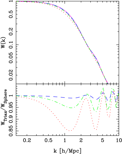
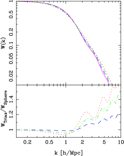
Figure 1: Variation of the window functions with increasing prolaticity. Left panels show effects for the continuity density profile model and right show the density profile model of JS02. In the top panels, the solid line represents spherical haloes, and the dash, dot-dash and dotted lines represent haloes with $a/c=b/c=0.8,\,0.6,\,0.4$ respectively. The bottom panels show the ratio of the window functions with the equivalent spherical haloes from each model and line styles have been preserved. In all cases the halo mass was set to be $M=1.0\times 10^{15}h^{-1}M\odot$.

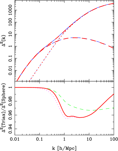
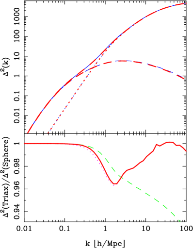
Figure 2: Dimensionless power spectrum in the triaxial halo model. Left panels show effects for the continuity profile model and right show the JS02 profile model. Top panels show: the total power spectrum (thick solid line); which is the sum of $P^{\rm 1H}$ (dotted lines) and $P^{\rm 2H}_{\rm NA}$ (dash lines); the total power from the spherical halo model (thin solid lines). Bottom panels show the ratios: total triaxial halo power to total spherical halo power (solid lines); triaxial 1-Halo to spherical 1-Halo (dotted lines); triaxial 2-Halo to spherical 2-Halo (dash lines).

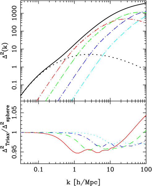
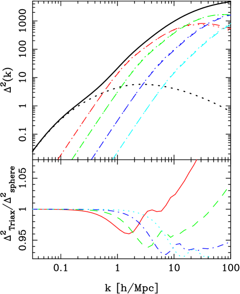
Figure 3: Contribution to the triaxial power spectrum from different mass ranges. Left panels show the continuity profile and the right show the JS02 profile model. Top panels, the dash-line and the dotted lines, going from left to right, show the contribution to the 1-Halo term for the mass ranges: $M>10^{14}h^{-1}M_{\odot}$; $10^{14}h^{-1}M_{\odot}\geq M>10^{13}h^{-1}M_{\odot}$; $10^{13}h^{-1}M_{\odot}\geq M>10^{12}h^{-1}M_{\odot}$; $10^{12}h^{-1}M_{\odot}\geq M>10^{11}h^{-1}M_{\odot}$. The thin dotted lines are the power spectrum split by mass for the equivalent spherical haloes. The thick dotted line is the 2-Halo term. Bottom panels show ratios of triaxial halo power to spherical for the same mass ranges as above, where we have adopted different and obvious line styles.

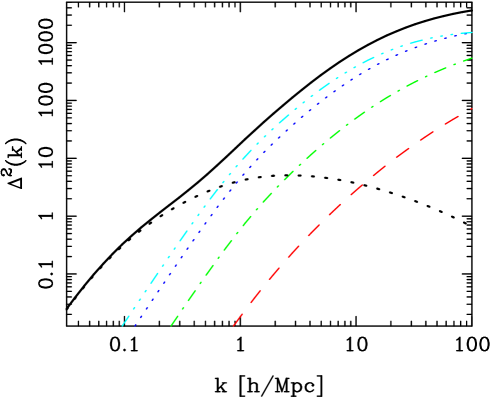
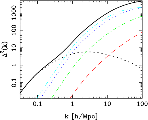
Figure 4: Similar to Fig. 3, but this time showing the break down of the power spectrum with axis ratio $a/c$. In both panels, we show, going up from the dash line to the triple-dot dash line, the contribution to the 1-Halo term coming from haloes with axis ratios: $1.0\geq a/c>0.85$; $0.85\geq a/c>0.7$; $0.7\geq a/c>0.55$; $0.55\geq a/c>0.3$. Again the left panel is the continuity model and the right is the JS02 model.

Figure 5: Contribution to the power spectrum from intrinsic alignments of the triaxial haloes, using the linear alignment model of equation (64). Left panel shows the variation with alignment normalization $\kappa_{0}$, and the right panel shows the variation with the power-law index $\epsilon$.

4 Results

4.1 Window functions & power spectra

In this Section, we present results for the numerical integration of the 1-Halo term’s window function, given by equation (30), and then the full power spectra given by equations (29), (35) and (43). However, before proceeding, we feel that it is necessary to mention the numerical algorithms we use to solve the equations.

Although our analytical efforts have reduced the dimensionality of the various power spectrum integrals dramatically, from 12- to 6-D for $P^{\rm 1H}$ and $P^{\rm 2H}_{\rm NA}$ and from 18- to 12-D for $P^{\rm 2H}_{\rm IA}$, the numerical integration of these equations using serial quadratures is extremely inefficient and intensely demanding on cpu time. We therefore recommend the use of an efficient multi-dimensional integrator, such as the Korobov-Conroy algorithm (Korobov, 1963; Conroy, 1967) or the Sag-Szekeres algorithm (Sag & Szekeres, 1964), both of which allow fast and accurate evaluations of these expressions (taking $\sim$10 minutes to evaluate equation (43) on a standard 2.8Ghz 32-bit Intel processor with heavy optimization afforded through the Intel compiler, and where the number of evaluation points in the Sag-Szekeres algorithm was set to 100 million). Both of the above algorithms have implementations vended through the Numerical Algorithms Group, listed as routines: d01fdf and d01gcf.

Figure 1 shows how, for the two different density profile models considered, the window functions, specified by equation (30), change as haloes become more prolate. From inspecting the top panels of these figures, it is clear that the overall effect is small. We therefore take the ratio of the window functions with those for the equivalent spherical model to inspect the effect more closely, where by equivalent spherical model we mean the window function for a particular triaxial profile model with $a/c=b/c=1$. For the continuity profile model (bottom left panel), we find that as the prolaticity increases, the ratio gets smaller. This relative suppression in the window function is maximal on scales of the order the virial radius of the halo, being at most $\sim$15% for the extreme, $a/c=0.4$, prolate objects. Considering the haloes with JS02 profiles (right panels), we find that the effect is first seen as a small suppression on large scales and then as an amplification on small scales. We ascribe this amplification to the fact that in the JS02 model $\delta_{e}^{c}$ increases as haloes become more ellipsoidal.

Figure 2 shows the total power spectrum in the triaxial halo model with no intrinsic alignments, obtained by the sum of equations (29) and (35). Note that here we plot the dimensionless power spectrum: $\Delta^{2}(k)=4\pi k^{3}P(k)/(2\pi)^{3}$ (Peacock, 1999). Considering the triaxial haloes with the continuity profile model (left panels), again the effect is weak. Looking at the ratio with the spherical case, we show that it is maximal on scales of the order the virial radius of clusters and is manifest as a suppression of power at the $\sim 5\%$ level. The oscillatory features that were seen in the window function have been washed out by averaging over the halo mass and axis ratio distributions. Considering the resultant power spectrum from the JS02 model (right panels), we find a similar overall effect as for the continuity model, with a suppression of the order $\sim 5\%$ on scales $k\sim 2h{\rm Mpc}^{-1}$. The oscillatory features seen in the window function again have been smoothed out and the small scale amplification is no longer apparent. For the case where haloes are not intrinsically aligned, we find differences between the spherical 2-Halo term and the triaxial of the order a few percent for both models. However, these effects occur on scales where the 2-Halo power is sub-dominant to the 1-Halo power and therefore can be neglected.

Figure 3, shows the contributions to the 1-Halo term from different mass ranges. For the continuity profile model (left panel), we find for each mass bin considered, that the power is suppressed relative to the spherical case, and that the effect is strongest for the high mass haloes, being at the level $\sim 6\%$. There is also an small amplification of power on small scales. For the JS02 profile model (right panel), we find that there is a characteristic de-amplification, followed by a strong amplification of power as one goes from large to small scales. Interestingly, the large-scale suppression of power is stronger for the lower mass haloes, being of the order $\sim 8\%$ for the $M\sim 5.0\times 10^{11}h^{-1}M_{\odot}$ objects on scales $k\sim 10h{\rm Mpc}^{-1}$. However, the small scale amplification effect is strongest for the high mass haloes, boosting the power to around $\sim 10\%$ for the $M\sim 10^{15}h^{-1}M_{\odot}$ on similar scales. Thus one sees that the largest effects of triaxiality are most apparent in the highest mass haloes. This result follows in accordance with the hierarchical picture of structure formation: high mass haloes form at late times in the Universe and thus particle orbits have insufficient time to circularize and hence structures are more likely to be triaxial than spherical. This effect is built into the JS02 probability density function through a mass dependent scaling of the stochastic variable $a/c$, which operates so that higher mass haloes are more likely to be triaxial than the lower mass haloes (see equations 16 and 17 in JS02). This indicates that if one is purly intersted in the clustering properties of extreme mass objects, then halo triaxiality plays a more significant role.

Figure 4 shows the contribution to the 1-Halo term from different ranges of the axis ratio $a/c$. Somewhat interestingly, in both cases, for $k<10\,h{\rm Mpc}^{-1}$ the power spectrum is entirely dominated by the most triaxial haloes, $a/c<0.7$, and that the spherical haloes contribute very little to the overall power. This observed effect: highly triaxial haloes contributing the most on large scales and spherical haloes accounting for more on small scales, can be understood entirely from the mass dependent scaling of the distribuion functions for $a/c$.

Figure 5 shows the contributions to the power spectrum from the 2-Halo intrinsic alignment term. We find that, for the linear correlation model specified by equation (64), the intrinsic alignments contribution to the power spectrum is, $\sim 10$ orders of magnitude smaller than the 2-Halo term with no alignmnets. As will become apparent from the following sub-section, this result is actually insensitive to our choices for $\kappa_{0}$ and $\epsilon$. Considering the variation of the clustering with $\kappa_{0}$ (left panel), we find that increasing/decreasing $\kappa_{0}$ simply uniformally increases/decreases $P^{\rm 2H}_{\rm IA}$. Next, considering the variation of the power with the power-law index $\epsilon$ (right panel), we find that as $\epsilon$ increases/decreases the alignment power spectrum decreases/increases, and that the variations are very similar to those with $\kappa_{0}$. This may mean that $\epsilon$ and $\kappa_{0}$ are not independent parameters.

4.2 Maximally alligned haloes

As a corollory to this section we discuss the limiting case of a maximally aligned halo distribution, that is, one in which the orientation vector of every halo is perfectly alligned with the others. Clearly, this scenario is unphysical, however it does allow us to place firm constraints on the largest possible contribution that alignments may provide. In order to achieve this we simply set the correlation function to be

$$C(\mu)=\delta^{D}(\mu\pm 1)-1\ \ ;\hskip 11.38092pt-1\leq\mu\leq 1\ .$$ (66)

In this limit we find that the function ${\mathcal{D}}$ in the intrinsic alignment term given by (equation 43) becomes

$${\mathcal{D}}(\theta_{k},\phi_{k}) = 4\pi\int d\psi\,\,{\rm j_{0}}\left[kR^{\prime}f(\theta_{k}^{\prime\prime},\phi_{k}^{\prime\prime})\right]$$ (67)

$$\ \ -\int d\alpha d(\cos\beta)d\gamma{\rm j_{0}}\left[kR^{\prime}f(\theta_{k}^{\prime},\phi_{k}^{\prime})\right],$$

where ${\bf k}^{\prime\prime}={\mathcal{R}}(0,0,\psi){\bf k}$ and ${\bf k}^{\prime}={\mathcal{R}}(\alpha,\beta,\gamma){\bf k}$, and where we have used the fact that for $\mu=\pm 1$, we may combine rotations over $\alpha$ and $\gamma$ into a new rotation over $\psi=\alpha-\gamma$.

Figure 6 shows the maximum possible contribution to the power spectrum from the intrinsic alignments of dark matter haloes that have the continuity density profile. We see that for this case, the alignment contribution has significantly increased by roughly $\sim 8-10$ orders of magnitude. However, relative to the total power (bottom panel), it is still a fairly small quantity, being at most an effect of the order $\sim 10\%$ on scales $k\sim 1\,h\,$Mpc^-1. Given that this alignment correlation function is physically unrealistic, we may now conclude that the true contribution to the power spectrum from alignments must be $<10\%$.

Figure 6: Maximal contribution to the power spectrum from intrinsic halo alignments. The top panel shows: the maximum alignments (cross hatched region defines the result $\pm$ the rms error); the 2-Halo term with no alignments (dash line); the 1-Halo term (dotted line); and the total contribution from all terms (thin solid line). The bottom panel shows the ratio of the maximum to the total power. The triaxial density profile model was the continuity model.

5 Discussion & Conclusions

In this paper we have developed a formalism for calculating the clustering statistics of a distribution of intrinsically aligned, triaxial, dark matter haloes: the triaxial halo model. This formalism facilitates the exploration of the importance of halo alignments and shapes on the density clustering statistics.

As a direct application of the formalism, we have considered the lowest order clustering statistic of interest, that is the power spectrum. We found, as usual, that the general result separates into a term that describes the clustering between haloes (2-Halo) and a term that describes the clustering within a halo (1-Halo). However, with the inclusion of intrinsic halo alignments we found that the 2-Halo term itself separates into two terms: the first described the halo-halo clustering without alignments; the second described the clustering due to halo alignments. We have derived compact analytic forms for these general relations, in all cases dramatically reducing the dimensionality of the integral equations. These were then solved numerically using two different multi-dimensional integrators. We considered two different density profile models. The first allowed us to explore pure shape effects on the clustering, the second was the more realistic profile model of JS02, which modified the halo central density based on halo shape. In both cases, we found that the effects on the power spectrum were, as expected, small, being at most $\sim 5\%$ for $k\sim 1-10h\,$Mpc^-1. However, when considerd by mass we found a more significant effect for the high mass objects, with a suppression of the order $\sim 6\%$ for the continuity model and an $\sim 5\%$ suppression of power on large scales followed by a $\sim 10-15\%$ amplification of power on small-scales for the JS02 model. The effects of halo triaxiality will be important to account for when interpreting precision measurements of cluster correlation functions on small scales. We have also found that the 1-Halo power is dominated by haloes with $a/c<0.7$.

We have explored the impact of halo alignments on the power spectrum. In order to achieve this it was necessary to develop a toy-model for the correlation function of the semi-major axis direction vectors of haloes. This model was constructed so that high mass haloes were more likely to be alligned than lower mass haloes. We further made the assumption that only haloes of the same mass are alligned. Although questionable, this assumption provided a means to consider the effects of a mass dependent alignmnet correlation function. For this model, we found that halo alignment contribution to the power spectrum was, surprisingly, $\sim 10$ orders of magnitude smaller than the 2-Halo term without alignments. Modifying the normalization parameters for the $C(\mu)$ does not significantly increase the alignment power. Thus, if our alignment model is correct halo alignments are completely unimportant for density clustering statistics.

We then constructed the maximal alignment correlation function. This allowed us to explore the physically unrealistic case where all haloes of all masses are completely alligned with one another. We found, for the triaxial haloes with the continuity profile, that the maximum alignment contribution to the power spectrum was $\sim 10\%$ on scales of the order $k\sim 1\,h\,$Mpc^-1 and significantly less on all other scales. This lead us to the conclusion that the true alignment contribution to the power must be $<10\%$.

We now add an important and necessary cautionary note. In order to make accurate predictions for the clustering in the triaxial halo model, we require an accurate model for the statistical properties of the triaxial dark matter haloes. Clearly, the first density profile model that we considered, the continuity model, was constructed simply as a toy-model, and as such the predictions should not be expected to match reality. In the second model, the JS02 model, the profiles were constructed to match results from numerical simulations. However, we have discovered some aspects of this model that should be clarified before it can be used with confidence to make accurate predictions for the clustering statistics.

Firstly, consider the special case of a halo that is actually spherical and apply the JS02 formalism to it, having obtained the two independent normalization parameters, we ask the question: At what radius does the average overdensity reach that at which we defined the halo? The answer is not the same as the virial radius that we defined from the mass. Secondly, the ellipsoidal concentration parameter $c_{e}\equiv R_{e}/R_{0}$ depends on the axis ratio $a/c$, and not the second ratio $b/c$. This leads to the following problem: When averaging over the axis ratio distributions, we found that whilst a haloes shape and characteristc density may change dramatically through changes in $b/c$, the concentration paramter remains fixed. This results in inconsistant density structures for the haloes, since we found that haloes of a given mass and $a/c$ could be less and more dense than spherical haloes, depending on the value of $b/c$. In reality it is more likely that haloes that are triaxial are either less dense, or of equivalent density, or more dense than spherical haloes, but not all. Whilst the model of JS02 is ground breaking in many ways, we feel in light of these problems that some aspects should be re-visited.

For the 1-Halo term we have found that modelling the density structure of haloes with triaxial ellipsoids produces an effect of the order $5-20\%$, relative to equivalently defined spherical haloes. For observational programs that hope to measure the small scale power spectrum to these levels of accuracy or better, one must therefore account for halo triaxiality when interpreting data with halo models.

We mentioned earlier that if one takes halo concentration to be a stochastic variable in the spherical halo model, then this too increases the small scale power (Cooray & Hu, 2001). The effect is thus degenerate with triaxiality for the JS02 haloes. If the main reason for the stochasticity of the halo concentration could be attributed to the incorrect assumption that haloes are spherical, then one might understand the degeneracy. However, JS02 found that there is a comparable scatter in the concentraion parameter for the ellipsoidal haloes as there is for the spherical. This they suggest is due to differences in the merger histories of the haloes and not asphericity.

A further effect on the small scale clustering that we have not yet mentioned is that of halo subtructures. The halo model formalism was extended to include this by Sheth & Jain (2003). Effects on the density power spectrum were then explored by Dolney, Jain & Takada (2004). They found that, in general, the small-scale clustering becomes dominated by substructures below a certain scale. The scale depends on the sub-structure mass function and density distribuiton. Again, the effect appears to be degenerate with the effects of triaxiality.

In this paper we have considered only the lowest order clustering statistics, the 2-pt auto-correalation function and the power spectrum. However, the overall goal of this work is to explore how the shapes of dark matter haloes and their intrinsic alignments influence the hierarchy of correlation functions. Since the 2-pt clustering statistics are the least sensative to the shapes of structures, it is not surprising that the degeneracies, noted above, have been found. However, it is expected that these will be broken through consideration of the higher order statistics, such as the bispectrum, and we will focus on this in a subsequent paper.

Appendix A Rotation matrix

Owing to there being several equivalent ways to define the Euler angles for the rotation matrix ${\mathcal{R}}(\alpha,\beta,\gamma)$, we make explicit the definition that we use throughout. The matrix for the $z-y^{\prime}-z^{\prime\prime}$ rotation is given by:

$${\mathcal{R}}(\alpha,\beta,\gamma)\equiv\left(\begin{array}[]{ccc}\rm c\,\beta\,\rm c\,\alpha\rm c\,\gamma&\rm c\,\beta\,\rm s\,\alpha\,\rm c\,\gamma&-\rm s\,\beta\,\rm c\,\gamma\\ -\rm s\,\alpha\,\rm s\,\gamma&+\rm c\,\alpha\,\rm s\,\gamma&\\ -\rm c\,\beta\,\rm c\,\alpha\,\rm s\,\gamma&-\rm c\,\beta\,\rm s\,\alpha\,\rm s\,\gamma&\rm s\,\beta\,\rm s\,\gamma\\ -\rm s\,\alpha\,\rm c\,\gamma&+\rm c\,\alpha\,\rm c\,\gamma&\\ \rm s\,\beta\,\rm c\,\alpha&\rm s\,\beta\,\rm s\,\alpha&\rm c\,\beta\\ \end{array}\right)\ ,$$ (68)

where we have adopted the short hand notation $\rm c=\cos$ and $\rm s=\sin$.

Appendix B The mass function and halo biasing

We model the mass function of dark matter haloes using the model of ST, since the predictions are in excellent agreement with the halo abundances measured directly from numerical simulations (ST Jenkins et al., 2001; Reed et al., 2003). The ST mass function is

$$\frac{dn(M)}{d\log M}=\frac{\bar{\rho}}{M}\;\nu f(\nu)\left|\frac{d\ln\nu}{d\ln M}\right|\ ;\ \ \nu\equiv\delta_{\rm col}/\sigma(M)\ ,$$ (69)

where

$$\nu f(\nu)=2A\left(1+\frac{1}{\nu^{\prime 2q}}\right)\left(\frac{\nu^{\prime 2}}{2\pi}\right)\exp\left(-\frac{\nu^{\prime 2}}{2}\right)\ ,$$ (70)

and where $\nu^{\prime}=\sqrt{a}\nu$, $a=0.707$, $q=0.3$ and $A\approx 0.322$. Sheth, Mo & Tormen (2000) argued that the success of the ST formula was due to the fact that the ellipsoidal model for halo collapse was more realistic, as opposed to the spherical.

We will also require a model for the halo biasing. Here we again look to the work of ST, who found

$$b(M)=1+\frac{a\nu^{2}-1}{\delta_{\rm col}}+\frac{2p/\delta_{\rm col}}{1+(a\nu^{2})^{p}}\ ;\ \ \ \nu\equiv\delta_{\rm col}/\sigma\ .$$ (71)

References

- Aldering et al. (2004) Aldering G., & The SNAP Team, 2004. astro-ph/0405232
- Bond & Efstatiou (1984) Bond J. R., Efstathiou G., 1984. ApJ, 285, 45.
- Bond et al. (1991) Bond J. R. , Cole S., Efstathiou G., Kaiser N., 1991. ApJ, 379, 440
- Bond & Myers (1996) Bond J. R., Myers S. T., 1996. ApJS, 103, 1
- Brown et al. (2002) Brown M. L., Taylor A. N., Hambly N. C., Dye S., 2002. MNRAS, 333, 501
- Chandrasekhar (1969) Chandrasekhar S., 1969. “Ellipsoidal figures of equilibrium“, Yale University Press, New Haven and London
- Colless et al. (2001) Colless M., & The 2dFGRS Team, 2001. MNRAS, 328, 1039
- Conroy (1967) Conroy H., 1967. J. Chem. Phys., 47, 5307
- Cooray & Hu (2001) Cooray A., Hu W., 2001. ApJ, 554, 56
- Cooray & Sheth (2003) Cooray A., Sheth R. K., 2003. Physics Reports, 372, 1
- Croft & Metzler (2000) Croft R., Metzler C., 2000. ApJ, 545, 561
- Dolney, Jain & Takada (2004) Dolney D., Jain B., Takada M., 2004, astro-ph/0401089
- Efstathiou, Bond & White (1992) Efstathiou G., Bond J. R., White S. D. M., 1992. MNRAS, 258, 1
- Eisenstein & Hu (1998) Eisenstein D., Hu W., 1998. ApJ, 496, 605.
- Gradshteyn & Ryzhik (1994) Gradshteyn I. S., Ryzhik I. M., 1994. “Table of integrals, series and products”, Fifth edition, Academic Press Inc., San Diego
- Hatton & Ninin (2001) Hatton S., Ninin S., 2001. MNRAS, 322, 576
- Hawkins et al. (2003) Hawkins E., & The 2dFGRS Team, 2003. MNRAS, 346, 78H
- Heavens, Refregier & Heymans (2000) Heavens A. F., Refregier A., Heymans C., 2000. MNRAS, 319, 649
- Heymans et al. (2004) Heymans C., Brown M. L., Heavens A. F., Meisenheimer K., Taylor A., Wolf C., 2004. MNRAS, 347, 895
- Hopkins, Bahcall & Bode (2004) Hopkins P., Bahcall N., Bode P., 2004. astro-ph/0409652
- Hoyle (1949) Hoyle F., 1949, in “Problems of Cosmical Aerodynamics”, in Problems of Cosmical Aerodynamics, J. M. Burgers & H. C. van de Hulst Paris eds., Central Air Documents Office, Dayton, p. 195
- Huffenberger & Seljak (2003) Huffenberger K., Seljak U., 2003. MNRAS, 340, 1199
- Jenkins et al. (2001) Jenkins A., Frenk C. S., White S. D. M, Colberg J. M., Cole S., Evrard A. E., Yoshida N., 2001. MNRAS, 321, 372
- Jing & Börner (2004) Jing Y. P., Börner G., 2004. ApJ, 607, 140
- Jing & Suto (2002) Jing Y. P., Suto Y., 2002. ApJ, 574, 538. (JS02)
- Jing (2002) Jing Y. P., 2002. MNRAS, 335, 89
- Kayo et al. (2004) Kayo I., & The SDSS Team, 2004. astro-ph/0403638
- Korobov (1963) Korobov N. M., 1963., “Number theoretic methods in approximate analysis”, Fizmatgiz, Moscow
- Lacey & Cole (1993) Lacey C., Cole S., 1993. MNRAS, 262, 627
- Lee & Pen (2001) Lee J., Pen U.-L., 2001. ApJ, 555, 106
- Mackey, White & Kamionkowski (2002) Mackey J., White M., Kamionkowski M., 2002. MNRAS, 332, 788
- Mathews & Walker (1970) Mathews J, Walker R. L., 1970. “Mathematical methods of physics”, W. A. Benjamin Publishers Inc., New York
- Ma & Fry (2000) Ma C., Fry J.N., 2000. ApJ, 543, 503
- McClelland & Silk (1977) McClelland J., Silk J., 1977. ApJ, 217, 331
- Mo & White (1996) Mo H-J., White S. D. M., 1996. MNRAS, 282, 347
- Navarro, Frenk & White (1997) Navarro J. F., Frenk C. S., White S. D. M., 1997. ApJ, 490, 493. (NFW)
- Oguri, Lee & Suto (2003) Oguri M., Lee J., Suto Y., 2003. ApJ, 599, 7
- Porciani, Dekel & Hoffman (2002) Porciani C., Dekel A., Hoffman Y., 2002. MNRAS, 332, 325
- Peacock & Smith (2000) Peacock J. A., Smith R. E., 2000. MNRAS, 318, 1144
- Peacock (1999) Peacock J. A., 1999. ”Cosmological Physics”, Cambridge University Press, Cambridge.
- Percival et al. (2001) Percival W., & The 2dFGRS Team, 2001. MNRAS, 327, 1297
- Reed et al. (2003) Reed D., Gardner J, Quinn T., Stadel J., Fardal M., Lake G., Governato, F., 2003. MNRAS, 346, 565
- Sag & Szekeres (1964) Sag T. W., Szekeres G., 1964. Math. Comput., 18, 254
- Scherrer & Bertschinger (1991) Scherrer R. J., Bertschinger E., 1991. ApJ, 381, 349
- Scoccimarro et al. (2001) Scoccimarro R., Sheth R. K., Hui L., Jain B., 2001. ApJ, 546, 20.
- Seljak & Zaldarriaga (1996) Seljak U., Zaldarriaga M., 1996. ApJ, 469, 437.
- Seljak (2000) Seljak U., 2000. MNRAS, 318, 203
- Sheth & Tormen (1999) Sheth R. K., Tormen G., 1999. MNRAS, 308, 119. (ST)
- Sheth, Mo & Tormen (2000) Sheth R. K., Mo H-J., Tormen G., 2000. MNRAS, 323, 1
- Sheth & Jain (2003) Sheth R. K., Jain B., 2003. MNRAS, 345, 592
- Smith et al. (2003) Smith R. E., Peacock J. A., Jenkins A. R., White S. D. M., Frenk C. S., Pearce F. R., Thomas P. A., Efstathiou G., Couchman H. M. P., 2003. MNRAS, 341, 1311
- Strauss et al. (2002) Strauss M., & The SDSS Team, 2002. AJ, 124, 1810
- Tegmark et al. (2004) Tegmark M., & The SDSS Team, 2004. ApJ, 606, 202
- Wang et al. (2000) Wang L., Caldwell R. R., Ostriker J. P., Steinhardt P. J., 2000. ApJ, 530, 17
- Zehavi et al. (2002) Zehavi I., & The SDSS Team, 2002. ApJ 571, 172