Correlated Primordial Perturbations in Light of CMB and LSS Data

Abstract

We use cosmic microwave background (CMB) and large-scale structure data to constrain cosmological models where the primordial perturbations have both an adiabatic and a cold dark matter (CDM) isocurvature component. We allow for a possible correlation between the adiabatic and isocurvature modes, and for different spectral indices for the power in each mode and for their correlation. We do a likelihood analysis with 11 independent parameters. We discuss the effect of choosing the pivot scale for the definition of amplitude parameters. The upper limit for the isocurvature fraction is 18% around a pivot scale $k=0.01$Mpc^-1. For smaller pivot wavenumbers the limit stays about the same. For larger pivot wavenumbers, very large values of the isocurvature spectral index are favored, which makes the analysis problematic, but larger isocurvature fractions seem to be allowed. For large isocurvature spectral indices $n_{\rm{iso}}>2$ a positive correlation between the adiabatic and isocurvature mode is favored, and for $n_{\rm{iso}}<2$ a negative correlation is favored. The upper limit to the nonadiabatic contribution to the CMB temperature variance is 7.5%. Of the standard cosmological parameters, determination of the CDM density $\omega_{c}$ and the sound horizon angle $\theta$ (or the Hubble constant $H_{0}$) are affected most by a possible presence of a correlated isocurvature contribution. The baryon density $\omega_{b}$ nearly retains its “adiabatic value”.

I Introduction

The major part of the present cosmological data, including the cosmic microwave background (CMB) anisotropy and the large scale distribution of galaxies (large scale structure, LSS) is fit reasonably well by a simple cosmological model. This model has a spatially flat ($\Omega=1$) background geometry. It has five energy density components, “baryons”, photons, massless neutrinos, cold dark matter (CDM), and a constant vacuum energy (cosmological constant). The primordial scalar perturbations are gaussian, adiabatic, and scale-free ($n_{\rm{ad}}=\mbox{const.}$).

We call this model the “adiabatic model” in this paper. It has 5 parameters to be determined from the data, the Hubble constant, $H_{0}\equiv h100\mbox{ km/s/Mpc}$, two density parameters, $\omega_{b}\equiv\Omega_{b}h^{2}$ and $\omega_{c}\equiv\Omega_{c}h^{2}$ (for baryons and CDM), and the amplitude $A$ and spectral index $n_{\rm{ad}}$ of the primordial scalar perturbations. There is no evidence in the cosmological data for the presence of additional features or ingredients beyond this model, like tensor perturbations or neutrino masses, indicating that they are probably so small as not to show up in the data. (Actually there is also no evidence for a deviation from scale-invariance, $n_{\rm{ad}}=1$.) The concordance values of the parameters are $h\sim 0.7$, $\omega_{b}\sim 0.023$, $\omega_{c}\sim 0.12$, $n_{\rm{ad}}\sim 1.0$, and $A\sim 5\times 10^{-5}$.

Besides these $5$ fundamental cosmological parameters, there are $2$ additional parameters needed when the models are compared to CMB and LSS data: the optical depth $\tau$ due to reionization, and the bias parameter $b$ relating the observed galaxy power spectrum to the underlying matter power spectrum.

The origin of the primordial perturbations is not known. The favorite candidate for their generation is quantum fluctuations during a period of inflation in the very early universe. While single-field inflation produces adiabatic perturbations, inflation with more than one field produces also entropy perturbations $\mathcal{S}$ in addition to the usual curvature perturbation $\mathcal{R}$.

A general perturbation can be divided into an adiabatic mode + an isocurvature mode, where the adiabatic mode has no initial entropy perturbation, and the isocurvature mode has no initial curvature perturbation. Allowing for the presence of an isocurvature mode does not improve the fit to the existing data (to the extent of justifying the additional parameters), and thus there is so far no evidence for the existence of primordial isocurvature perturbations. However, it is of interest to find out what limits the data set to these perturbations, as the nature of primordial perturbations is an important clue to their origin. Moreover, the presence of an undetected isocurvature contribution may affect the determination of the main cosmological parameters.

In principle, there can be different kinds of entropy perturbations, and thus several different isocurvature modes. Four different isocurvature modes were identified in Bucher et al. (2000), the CDM and baryon isocurvature modes, and two neutrino isocurvature modes. Allowing for the simultaneous presence of all four kinds would lead to so many parameters that it would be difficult to obtain meaningful results Bucher et al. (2001). The signature of a baryon isocurvature mode in the data is rather similar to the CDM isocurvature mode, but weaker due to the smaller baryon density parameter.

Here we consider only the CDM isocurvature mode in addition to the adiabatic mode. We allow the CDM entropy perturbations to have a different spectral index from the curvature perturbations, and to be (or not to be) correlated with them. In comparison to the adiabatic model this brings in 4 new parameters related to the amplitudes and spectral indices of the entropy perturbations and their correlation with the curvature perturbations. Thus we have in total $11$ parameters in our cosmological model. For sampling this 11-dimensional parameter space we use the Markov Chain Monte Carlo (MCMC) method. This is a follow-up paper of Valiviita and Muhonen (2003) where a preliminary analysis (around the best-fit adiabatic model) was presented. Here we include more data in the analysis and sample the likelihood function more accurately.

Before the Wilkinson Microwave Anisotropy Probe (WMAP) data Bennett et al. (2003) became available, limits to the isocurvature contribution in uncorrelated models had been obtained for the case $n_{\rm{ad}}=n_{\rm{iso}}=1$ in Stompor et al. (1996) and with $n_{\rm{ad}}$ and $n_{\rm{iso}}$ as independent parameters in Enqvist et al. (2000), and in correlated models for one independent spectral index in Amendola et al. (2002). Pure CDM isocurvature models had been ruled out also in the case of a non-flat background geometry in Enqvist et al. (2002). Correlated models were also studied in Moroi and Takahashi (2001, 2002).

After WMAP, limits to correlated models were first obtained for the case of two independent spectral indices Peiris et al. (2003); Crotty et al. (2003). In our earlier work Valiviita and Muhonen (2003) we obtained preliminary results for the case of three independent spectral indices using WMAP data only. Parkinson et al. Parkinson et al. (2004) considered a particular inflation model producing correlated perturbations. Moodley et al. Moodley et al. (2004) considered models with up to three isocurvature modes (CDM and two neutrino modes) present simultaneously, but all sharing the same spectral index. Ferrer et al. Ferrer et al. (2004) studied correlated perturbations resulting from inflaton and curvaton decay. They had two independent spectral indices.

The most similar to the present study is that of Beltran et al. Beltran et al. (2004), who consider one isocurvature mode at a time, and allow separate spectral indices for the adiabatic and isocurvature modes and their correlation. We compare their approach to ours at the end of Sec. II and their results to ours in Sec. VII.

Since the adiabatic and isocurvature components and their correlation are allowed to have different spectral indices, their relative amplitudes vary as a function of scale $k$. We define the amplitude parameters at some chosen pivot scale $k_{0}$.

When the isocurvature component or the correlation is negligibly small, the corresponding spectral indices are not constrained by the data. Such conditionally unconstrained parameters cause problems also for determining other parameters from the data.

The way the isocurvature perturbation and correlation is parameterized (e.g. the choice of pivot scale $k_{0}$) affects the integration measure in the parameter space. Thus different parameterizations correspond to different priors. When parameters are weakly constrained by the data this ends up in different posterior likelihoods: When one parametrization (A) is used to obtain the likelihood function in the parameter space and the results are then expressed in another parametrization (B), the likelihood function is different from the case when parametrization B was used initially. (This difference can be “fixed” by importance weighting using the Jacobian of the parameter transformation; but this does not address the question which parametrization is “correct”.) Such effects are discussed in Sec. VI.

We find that the pivot scale should be chosen to be near the middle of the data sets used (in terms of $\ln k$). When the isocurvature spectral index $n_{\rm{iso}}$ is a free parameter a wrong choice would spoil the analysis. This comes because the data does not prefer an isocurvature contribution. Then using $k_{0}$ that is close to the small $k$ end of the data, $k_{\mathrm{min}}$, leads to extremely small (negative) $n_{\rm{iso}}$, in order to minimize the isocurvature contribution. On the other hand, if $k_{0}$ is too close to $k_{\mathrm{max}}$, then arbitrarily large isocurvature spectral indices are favored to minimize an overall isocurvature contribution in the range $[k_{\mathrm{min}},k_{\mathrm{max}}]$. Unfortunately, the “standard pivot scale” $k_{0}=0.05$Mpc^-1 (used e.g. by CAMB Lewis and Bridle (2002); Lewis et al. (2000)) is quite close to $k_{\mathrm{max}}$ and another common choice (see e.g. Crotty et al. (2003)) to give for $k_{0}$ a value that corresponds to the present Hubble radius is nearly equal to setting $k_{0}=k_{\mathrm{min}}$.

When we started MCMC runs for our model we took $k_{0}=0.05$Mpc^-1, but soon realized that our Markov Chains ran towards artificially large $n_{\rm{iso}}$. After fixing this problem, when we were finalizing the analysis of better runs with $k_{0}=0.01$Mpc^-1, paper Beltran et al. (2004) with pivot scale $k_{0}=0.05$Mpc^-1 came out. However, they had an ad hoc constraint $n_{\rm{iso}}<3$ that saved their main results from most of the artifacts that arise when the chains run to very large $n_{\rm{iso}}$. With our choice of the pivot scale the likelihood for $n_{\rm{iso}}$ peaks at $n_{\rm{iso}}\sim 3$ and drops rapidly around $n_{\rm{iso}}\sim 4$. Hence, the prior $n_{\rm{iso}}<3$ in Beltran et al. (2004) allows a comparison to our results.

We obtain tight constraints to the CDM isocurvature contribution and find that, of the main cosmological parameters, only the determination of $\omega_{c}$ and $h$ is significantly affected. Compared to the adiabatic models smaller values of $\omega_{c}$ and larger values of $h$ become acceptable when allowing for CDM isocurvature. Interestingly, although we have two additional degrees of freedom in spectral indices, dertermination of the baryon density is much less affected than in the models where all modes share the same spectral index.

In Sec. II we introduce and motivate our parametrization of correlated curvature and entropy perturbations. In Sec. III we write down some technical details of our MCMC study to determine these parameters, and in Sec. IV we give and discuss our results. In Sec. V we discuss the non-adiabatic contribution to the observed CMB and matter power spectra, and in Sec. VI the effect of changing the pivot scale. In Sec. VII we compare our results to those of Beltran et al. (2004).

II Correlated Perturbations

The calculation of the CMB angular power spectra $C_{l}$ and the matter power spectra $P(k)$ starts from “initial” values $\mathcal{R}_{\mathrm{rad}}$ and $\mathcal{S}_{\mathrm{rad}}$ specified deep in the radiation dominated era (rad), when all scales of interest are well “outside the horizon” (i.e., the Hubble scale $H^{-1}$). However, this “initial” time is well after inflation, or whatever generated the perturbations, and refers to a time during and after which the evolution of the universe is assumed to be known. We denote the time when the perturbations were generated by the subscript $\ast$. For inflation, this corresponds to the time when the scale in question “exited the horizon” (thus it is different for different scales $k$). Between $t_{\ast}(k)$ and $t_{\mathrm{rad}}$ the perturbation is outside the horizon, i.e., $k$ is “superhorizon”.

In the absence of entropy perturbations, curvature perturbations remain constant at superhorizon scales. This is not, in general, true for entropy perturbations, which may evolve at superhorizon scales. Entropy perturbations may also seed curvature perturbations. This happens, e.g., in two-field inflation, when the background trajectory in field space is curved Langlois (1999); Langlois and Riazuelo (2000); Gordon et al. (2001).

Thus the relation between the “generated” and “initial” values for $\mathcal{R}$ and $\mathcal{S}$ can be represented as Amendola et al. (2002)

$$\begin{pmatrix}\mathcal{R}_{\mathrm{rad}}\\ \mathcal{S}_{\mathrm{rad}}\end{pmatrix}=\begin{pmatrix}1&T_{\mathcal{RS}}\\ 0&T_{\mathcal{SS}}\end{pmatrix}\begin{pmatrix}\mathcal{R}_{\ast}\\ \mathcal{S}_{\ast}\end{pmatrix}.$$ (1)

The transfer functions $T_{xy}(k)$ describe how the perturbations evolve from the time of inflation to the beginning of the radiation dominated era. The exact form of these functions is model dependent and that aspect is not studied in this work. We approximate them by power laws.

In the literature there are different sign conventions for the perturbations ${\mathcal{R}}$ and ${\mathcal{S}}$. We define them so that an initial positive comoving curvature perturbation $\mathcal{R}_{\mathrm{rad}}$ corresponds to an initial overdensity $\delta=\delta\rho/\rho>0$, and an initial positive entropy perturbation $\mathcal{S}_{\mathrm{rad}}$ corresponds to an initial CDM overdensity. In terms of the Bardeen potentials, $\Phi$ and $\Psi$, defined so that the metric in the conformal-Newtonian gauge is

$$ds^{2}=-(1+2\Phi)dt^{2}+a(t)^{2}(1-2\Psi)\delta_{ij}dx^{i}dx^{j}\,,$$ (2)

the comoving curvature perturbation reads

$$\mathcal{R}\equiv-\Psi-\frac{2\rho}{3(\rho+p)}\left(\frac{1}{H}\frac{\partial\Psi}{\partial t}+\Phi\right)\,,$$ (3)

and the entropy perturbation is

$$\mathcal{S}\equiv\delta_{c}-\frac{3}{4}\delta_{\gamma}\,,$$ (4)

where $\delta_{c}$ and $\delta_{\gamma}$ are the CDM and photon density perturbations. With these sign conventions, the ordinary Sachs-Wolfe effect is

$$\frac{\delta T}{T}\approx-\frac{1}{5}(\mathcal{R}_{\mathrm{rad}}+2f_{c}\mathcal{S}_{\mathrm{rad}})$$ (5)

(here $f_{c}\equiv\omega_{c}/(\omega_{b}+\omega_{c})$), and a positive correlation between $\mathcal{R}_{\mathrm{rad}}$ and $\mathcal{S}_{\mathrm{rad}}$ leads to an additional positive contribution to the large scale CMB anisotropy, and also to a positive contribution to the matter power spectrum.

We define the correlation $\mathcal{C}_{xy}(k)$ between two perturbation quantities (random variables), $x$ and $y$, as

$$\bigl{\langle}x(\vec{k})y^{\ast}(\vec{k}^{\prime})\bigr{\rangle}\bigr{|}_{\mathrm{rad}}=\tfrac{2\pi^{2}}{k^{3}}\mathcal{C}_{xy}(k)\delta^{(3)}(\vec{k}-\vec{k}^{\prime}).$$ (6)

The transfer function $T_{\mathcal{RS}}(k)$ leads to a correlation between $\mathcal{R}_{\mathrm{rad}}$ and $\mathcal{S}_{\mathrm{rad}}$ from uncorrelated $\mathcal{R}_{\ast}$ and $\mathcal{S}_{\ast}$,

$$\mathcal{C}_{\mathcal{RR}}(k) =\mathcal{P}_{\mathcal{R}}(\ast,k)+T_{\mathcal{RS}}(k)^{2}\mathcal{P}_{\mathcal{S}}(\ast,k)$$ (7)

$$\mathcal{C}_{\mathcal{RS}}(k) =T_{\mathcal{RS}}(k)T_{\mathcal{SS}}(k)\mathcal{P}_{\mathcal{S}}(\ast,k)$$ (8)

$$\mathcal{C}_{\mathcal{SS}}(k) =T_{\mathcal{SS}}(k)^{2}\mathcal{P}_{\mathcal{S}}(\ast,k)\,,$$ (9)

where $\mathcal{P}_{\mathcal{R}}(\ast,k)$ and $\mathcal{P}_{\mathcal{S}}(\ast,k)$ are the power spectra of $\mathcal{R}_{\ast}$ and $\mathcal{S}_{\ast}$.

Approximating the power spectra $\mathcal{P}_{\mathcal{R}}(\ast,k)$, $\mathcal{P}_{\mathcal{S}}(\ast,k)$ and the transfer functions $T_{\mathcal{RS}}(k)$, $T_{\mathcal{SS}}(k)$ by power laws with spectral indices $m_{1}$, $m_{2}$, $m_{3}$, and $m_{4}$, respectively, we get that the autocorrelations (power spectra) have the form

$$\begin{split}\mathcal{P}_{\mathcal{R}}(k)&\equiv\mathcal{C}_{\mathcal{RR}}(k)=A^{2}_{r}\biggl{(}\frac{k}{k_{0}}\biggr{)}^{n_{\rm{ad1}}-1}+A^{2}_{s}\biggl{(}\frac{k}{k_{0}}\biggr{)}^{n_{\rm{ad2}}-1}\\ \mathcal{P}_{\mathcal{S}}(k)&\equiv\mathcal{C}_{\mathcal{SS}}({k})=B^{2}\biggl{(}\frac{k}{k_{0}}\biggr{)}^{n_{\rm{iso}}-1},\end{split}$$ (10)

where $n_{\rm{ad1}}=m_{1}+1$, $n_{\rm{ad2}}=m_{2}+2m_{3}+1$, and $n_{\rm{iso}}=m_{2}+2m_{4}+1$ and the epoch (rad) is implied. The three components are the usual adiabatic mode, a second adiabatic mode generated by the entropy perturbation, and the usual isocurvature mode, with amplitudes $A_{r}$, $A_{s}$ and $B$ at the pivot scale $k=k_{0}$, respectively.

The cross-correlation between the adiabatic and the isocurvature component is now

$$\mathcal{C}_{\mathcal{RS}}(k)=\mathcal{C}_{\mathcal{SR}}(k)=A_{s}B\biggl{(}\frac{k}{k_{0}}\biggr{)}^{n_{\rm{cor}}-1},$$ (11)

where $n_{\rm{cor}}=m_{2}+m_{3}+m_{4}+1=(n_{\rm{iso}}+n_{\rm{ad2}})/2$. The correlation is between the second adiabatic and the isocurvature component as is natural since these components have the same source.

We have chosen the pivot scale $k_{0}=0.01\leavevmode\nobreak\ \mbox{Mpc}^{-1}$, but we also consider pivot scales 0.002 Mpc^-1 and 0.05 Mpc^-1 in Sec. VI. We shorten the notation by defining ${\bar{k}}=k/k_{0}$.

The CMB angular power spectrum is given by

$$C_{l}^{(\mathrm{T/E/B})(\mathrm{T/E/B})}=\\ 4\pi\sum_{xy}\int\frac{dk}{k}\mathcal{C}_{xy}(k)g^{(\mathrm{T/E/B})}_{xl}(k)g^{(\mathrm{T/E/B})}_{yl}(k),$$ (12)

where the $g_{l}$’s are the transfer functions that describe how an initial perturbation evolves to a temperature (T) or polarization (E- or B-mode) anisotropy multipole $l$.

Now, using the equations (10), (11) and (12) we obtain for the temperature angular power spectrum

$$C^{\mathrm{TT}}_{l} =4\pi\int\frac{dk}{k}\Bigl{[}A^{2}_{r}\bigl{(}g^{\mathrm{T}}_{\mathcal{R}\>l}\bigr{)}^{2}{\bar{k}}^{n_{\rm{ad1}}-1}+A^{2}_{s}\bigl{(}g^{\mathrm{T}}_{\mathcal{R}\>l}\bigr{)}^{2}{\bar{k}}^{n_{\rm{ad2}}-1}$$

$$\quad+B^{2}\bigl{(}g^{\mathrm{T}}_{\mathcal{S}\>l}\bigr{)}^{2}{\bar{k}}^{n_{\rm{iso}}-1}+2A_{s}Bg^{\mathrm{T}}_{\mathcal{R}\>l}g^{\mathrm{T}}_{\mathcal{S}\>l}{\bar{k}}^{n_{\rm{cor}}-1}\Bigr{]}$$

$$\equiv A_{r}^{2}\hat{C}^{\mathrm{TTad1}}_{l}+A_{s}^{2}\hat{C}^{\mathrm{TTad2}}_{l}+B^{2}\hat{C}^{\mathrm{TTiso}}_{l}+A_{s}B\hat{C}^{\mathrm{TTcor}}_{l},$$ (13)

and for the TE cross-correlation spectrum

$$C^{\mathrm{TE}}_{l} =4\pi\int\frac{dk}{k}\Bigl{[}A^{2}_{r}g^{\mathrm{T}}_{\mathcal{R}\>l}g^{\mathrm{E}}_{\mathcal{R}\>l}{\bar{k}}^{n_{\rm{ad1}}-1}+A^{2}_{s}g^{\mathrm{T}}_{\mathcal{R}\>l}g^{\mathrm{E}}_{\mathcal{R}\>l}{\bar{k}}^{n_{\rm{ad2}}-1}$$

$$\quad+B^{2}g^{\mathrm{T}}_{\mathcal{S}\>l}g^{\mathrm{E}}_{\mathcal{S}\>l}{\bar{k}}^{n_{\rm{iso}}-1}$$

$$\quad+A_{s}B\bigl{(}g^{\mathrm{T}}_{\mathcal{R}\>l}g^{\mathrm{E}}_{\mathcal{S}\>l}+g^{\mathrm{T}}_{\mathcal{S}\>l}g^{\mathrm{E}}_{\mathcal{R}\>l}\bigr{)}{\bar{k}}^{n_{\rm{cor}}-1}\Bigr{]}$$

$$\equiv A_{r}^{2}\hat{C}^{\mathrm{TEad1}}_{l}+A_{s}^{2}\hat{C}^{\mathrm{TEad2}}_{l}+B^{2}\hat{C}^{\mathrm{TEiso}}_{l}+A_{s}B\hat{C}^{\mathrm{TEcor}}_{l}\,.$$ (14)

There are thus $3$ amplitude parameters (three absolute values and one sign, the relative sign of $A_{s}$ and $B$.) Now we need to choose the amplitude parametrization to be used in the likelihood analysis, i.e., what shall we use as the three independent parameters with flat prior likelihoods. One choice would be just $A_{r}$, $A_{s}$, and $B$. However, we would rather express our results in terms of a total amplitude, a relative isocurvature contribution and a correlation.

In Valiviita and Muhonen (2003) we followed Peiris et al. (2003) and used

$$f_{\mathrm{iso}}\equiv\sqrt{\frac{B^{2}}{A_{r}^{2}+A_{s}^{2}}}\in[0,\infty)$$ (15)

for the isocurvature contribution and

$$\cos\Delta\equiv{\mbox{sign}}(A_{s}B)\sqrt{\frac{A_{s}^{2}}{A_{r}^{2}+A_{s}^{2}}}$$ (16)

for the correlation (with the sign convention opposite to that of Peiris et al. (2003)). The data is quadratic in these parameters (see Eq. (II)), meaning that fairly large values of $f_{\mathrm{iso}}$ and $\cos\Delta$ are needed for the effect to show up in the data. This exacerbates the problem that models with a small $A_{s}$ and $B$ get a lot of weight in the likelihood function, since the spectral indices $n_{\rm{ad2}}$ and $n_{\rm{iso}}$ are not constrained.

A flat prior for $\cos\Delta$ leads to a non-flat prior distribution for $\cos^{2}\!\!\Delta$. Thus the parametrization by $\cos\Delta$ favors small multiplier $\cos^{2}\!\!\Delta$ in front of the second adiabatic component in Valiviita and Muhonen (2003); Peiris et al. (2003). Moreover, large values of $\sin^{2}\!\!\Delta=1-\cos^{2}\!\!\Delta$ are then favored, so that even without any data the first adiabatic component will be favored in the likelihood analysis. Likewise, the parametrization by $f_{\mathrm{iso}}$ (instead of $f_{\mathrm{iso}}^{2}$) favor small multiplier in front of the isocurvature component. All in all, there was an implicit bias towards pure adiabatic models in Valiviita and Muhonen (2003); Peiris et al. (2003). A similar caveat applies to Ferrer et al. (2004).

We would prefer amplitude parameters for which the data has a linear response. We define a total amplitude parameter $A$ by

$$A^{2}\ \equiv\ A_{r}^{2}+A_{s}^{2}+B^{2}$$ (17)

and the isocurvature fraction and correlation parameters

$$\alpha \equiv\frac{B^{2}}{A^{2}}\in[0,1]$$ (18)

$$\gamma \equiv{\mbox{sign}}(A_{s}B)\frac{A_{s}^{2}}{A_{r}^{2}+A_{s}^{2}}\in[-1,1]\,.$$ (19)

Now the total angular power spectrum can be written as:

$$C_{l} =A^{2}\bigl{[}(1-\alpha)(1-|\gamma|)\hat{C}^{\mathrm{ad1}}_{l}+(1-\alpha)|\gamma|\hat{C}^{\mathrm{ad2}}_{l}$$

$$+\alpha\hat{C}^{\mathrm{iso}}_{l}+\mathrm{sign}(\gamma)\sqrt{\alpha(1-\alpha)|\gamma|}\hat{C}^{\mathrm{cor}}_{l}\bigr{]}$$

$$\equiv C^{\mathrm{ad1}}_{l}+C^{\mathrm{ad2}}_{l}+C^{\mathrm{iso}}_{l}+C^{\mathrm{cor}}_{l}\,.$$ (20)

Here $\hat{C}^{\mathrm{ad1}}_{l}$ and $\hat{C}^{\mathrm{ad2}}_{l}$ represent adiabatic spectra which would result from a curvature perturbation $\mathcal{R}_{\mathrm{rad}}$ with unit amplitude ($A_{r}=1$ or $A_{s}=1$) at the pivot scale $k_{0}$. (They are otherwise the same, but have spectral indices $n_{\rm{ad1}}$ and $n_{\rm{ad2}}$.) Likewise, $\hat{C}^{\mathrm{iso}}_{l}$ represents an isocurvature spectrum from a CDM entropy perturbation of unit amplitude ($B=1$), and $\hat{C}^{\mathrm{cor}}_{l}$ the extra contribution from correlation for $A_{s}B=1$. (See Figs. 1 and 2, which represent the case of scale-invariant perturbations.). The “hatless” $C^{\mathrm{ad1}}_{l}$, $C^{\mathrm{ad2}}_{l}$, $C^{\mathrm{iso}}_{l}$, which are necessarily non-negative, and $C^{\mathrm{cor}}_{l}$, which can also be negative, are the contributions to the total $C_{l}$. A relation similar to (II) holds for the matter power spectrum $P(k)$.

Note that, e.g., $\alpha=0.5$ does not mean that the adiabatic and isocurvature contributions would be equal at any particular scale. Since $\alpha$ refers to the ratio of primordial perturbations, to which the $C_{l}$ contributions are related through the transfer functions, the situation is different for different scales, and depends on the other cosmological parameters. In particular, if the spectral indices are very different, a very small isocurvature fraction can still correspond to a large isocurvature contribution at some scales and vice versa.

We define a shorthand notation

$$\alpha_{\mathrm{cor}}\equiv\mathrm{sign}(\gamma)\sqrt{\alpha(1-\alpha)|\gamma|}$$ (21)

for the relative “weight” of the correlation spectrum $C^{\mathrm{cor}}_{l}$.

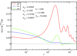
Figure 1: The unit-amplitude component angular power spectra $\hat{C}^{\mathrm{ad}}_{l}$ (red), $\hat{C}^{\mathrm{iso}}_{l}$ (blue), and $\hat{C}^{\mathrm{cor}}_{l}$ (green) of Eqs. (II) and (II) for the case of spectral indices $n_{\rm{ad}}=n_{\rm{iso}}=1$ and other cosmological parameters representing median values of their marginalized likelihoods from our 11-parameter model. These curves would represent the relative contributions to the total $C_{l}$ for the case $\alpha=0.5$, $\gamma=1$, i.e., “equal” weights for the adiabatic and isocurvature contributions and a maximal positive correlation between them.

The problem remains that when some multiplier in (II) is close to zero, the spectral index of the corresponding component becomes unconstrained leading to more volume in parameter space upon marginalization. This may introduce a bias towards “pure” models where the isocurvature or correlation amplitude is zero.

We want the pivot scale to be roughly in the middle of the data set used, and have chosen $k_{0}=0.01\mbox{Mpc}^{-1}$ as our pivot wavenumber. For the concordance values of the cosmological parameters, $\Omega_{\Lambda}=h=0.7$, this corresponds to “pivot multipole” $l_{0}\sim 140$. [The correspondence is $l_{0}\sim D_{\ast}k_{0}$, where $D_{\ast}=D_{\ast}(h,\Omega_{\Lambda},\Omega_{m})$ is the angular diameter distance to last scattering. $D_{\ast}(h,0.7,0.3)\approx h^{-1}$10 000Mpc^-1 while the “old day’s standard value” was $D_{\ast}(h,0,1)\approx h^{-1}$6 000Mpc^-1.]

This work is similar to a recently published study by Beltran et al. Beltran et al. (2004). The main differences are: 1) Different parametrization of correlation. When we divide the adiabatic spectrum in a correlated and an uncorrelated part, they consider the total adiabatic spectrum $\mathcal{P}_{\mathcal{R}}$ and the correlation spectrum $\mathcal{C}_{\mathcal{RS}}$ as the basic entities, which they approximate by power laws. This leads to constraints on the correlation spectral index $n_{\rm{cor}}$, which depend on the correlation amplitude, and therefore they introduce a related parameter, “$\delta_{\mathrm{cor}}$”, to be the independent parameter, leaving $n_{\rm{cor}}$ as a derived parameter. 2) They have set an upper limit $n_{\rm{iso}}\leq 3$, whereas we allow $n_{\rm{iso}}$ to vary over a wider range. 3) They use a pivot scale $k_{0}=0.05\mbox{ Mpc}^{-1}$ ($l_{0}\sim 700$). We use $k_{0}=0.01\mbox{ Mpc}^{-1}$ ($l_{0}\sim 140$), but consider also the effect of changing the pivot scale. 4) They use a larger data set, including type Ia Supernova (SNIa) data Riess et al. (2004), whereas we use CMB and LSS data only.

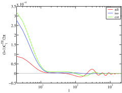
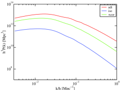
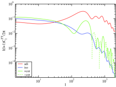
Figure 2: The same as Fig. (1), but for (a) $\hat{C}_{l}^{\mathrm{TE}}$ and (b) the matter power spectrum $\hat{P}(k)$. We also show (c) the $\hat{C}_{l}^{\mathrm{TT}}$ of Fig. 1 with a logarithmic scale, so that the effect of changing the spectral indices can be readily estimated from the figure. The pivot scale $k_{0}=0.01\mbox{Mpc}^{-1}$ becomes $k_{0}/h=0.01418$Mpc^-1 for the parameter values used ($h=0.7053$) for this plot.

5) They include an equation-of-state parameter $w$ for dark energy, wheras we keep $w=-1$. 6) They consider neutrino isocurvature modes also.

Crotty et al. Crotty et al. (2003) and Beltran et al. Beltran et al. (2004) use the same isocurvature parameter $\alpha$ as we use, but they use the correlation parameter

$$\beta\equiv-\cos\Delta\equiv\!-{\mbox{sign}}(A_{s}B)\sqrt{\frac{A_{s}^{2}}{A_{r}^{2}+A_{s}^{2}}}\equiv\!-{\mbox{sign}}(\gamma)\sqrt{|\gamma|}$$ (22)

In Crotty et al. (2003) $\beta$ is assumed scale invariant, whereas in Beltran et al. (2004) it is approximated by a power law with index $n_{\rm{cor}}$ so that our $n_{\rm{cor}}\equiv\frac{1}{2}(n_{\rm{ad2}}+n_{\rm{iso}})$ corresponds to their $n_{\rm{cor}}+\frac{1}{2}(n_{\rm{ad}}+n_{\rm{iso}})$.

III Technical Details of the Analysis

The model we are studying has 11 parameters. We have chosen to use the following independent parameters (primary parameters) for the likelihood analysis: the baryon density $\omega_{\mathrm{b}}$, the CDM density $\omega_{\mathrm{c}}$, the sound horizon angle $\theta$, the optical depth due to reionization $\tau$, the bias parameter $b$, the uncorrelated adiabatic spectral index $n_{\rm{ad1}}$, the correlated adiabatic spectral index $n_{\rm{ad2}}$, the isocurvature spectral index $n_{\rm{iso}}$, the logarithm of the overall amplitude $\ln(10^{10}A^{2})$, the isocurvature fraction $\alpha$ and the correlated fraction $\gamma$ of the adiabatic perturbations.

The sound horizon angle (in units of $\frac{1}{100}$ radian)

$$\theta=\theta(\omega_{b},\omega_{c},h)\equiv 100\times\frac{s_{\ast}}{D_{\ast}}\,,$$ (23)

where $s_{\ast}$ is the sound horizon at last scattering and $D_{\ast}$ is the angular diameter distance to last scattering Hu et al. (2001), is used as an independent parameter instead of $h$ (or $\Omega_{\Lambda}$), since it is more tightly constrained by the data.

The bias $b$ is defined by

$$\left.\phantom{\Big{(}}P_{\mathrm{gal}}^{\mathrm{SDSS}}(k)\right|_{z_{\mathrm{eff}}\simeq 0.15}=\left.\phantom{\Big{)}}b^{2}P(k)\right|_{z=0}\,.$$ (24)

So we multiply the present-day theoretical matter power $P(k)$ by $b^{2}$ before comparing to the galaxy power spectrum observed by the Sloan Digital Sky Survey (SDSS) Tegmark et al. (2004a) at effective redshift $z_{\mathrm{eff}}$. In the figures, we actually plot $b^{2}P(k)$.

We find the posterior likelihoods for the primary parameters and a number of derived parameters using the Markov Chain Monte Carlo (MCMC) method. The chains are generated using our modified version of the publicly available CosmoMC code Lewis and Bridle (2002). The CMB angular power spectra and the matter power spectra are calculated by the CAMB code Lewis et al. (2000); Lewis and Challinor (2002) (see also Gordon and Lewis (2003)). It needed some modifications for faster treatment of correlation.

CosmoMC/CAMB evaluates the matter power spectrum in linear perturbation theory. However, very small scales ($k/h\gtrsim 0.15$Mpc^-1) have already become non-linear. The publicly available code HALOfit utilizes results from lattice simulations of clustering Smith et al. (2003). However, the applicability of the HALOfit to our model is not granted, since the lattice simulations have been performed in adiabatic models with moderate spectral indices. Hence, following the recipe of Tegmark et al. (2004a), we calculate the matter power spectra in linear theory and compare them only to the first 17 data points ($k/h\lesssim 0.15$Mpc^-1) of the SDSS galaxy survey Tegmark et al. (2004a).

For the observational CMB data we take the WMAP temperature autocorrelation (TT) and temperature-polarization cross-correlation (TE) data Hinshaw et al. (2003); Kogut et al. (2003); Verde et al. (2003). To extend the coverage of the data to higher multipoles we use the TT data from CBI Readhead et al. (2004) and ACBAR Kuo et al. (2004), which we later call “other CMB data”.

Details of the data sets are:

• WMAP TT, 899 data points, $l=2$ – $900$,
  ($k\sim 1.4\times 10^{-4}$Mpc^-1 – $0.064$Mpc^-1).

• WMAP TE, 449 data points $l=2$ – $450$,
  ($k\sim 1.4\times 10^{-4}$Mpc^-1 – $0.032$Mpc^-1).

• ACBAR TT, 7 $l$-bands, $l_{\rm eff}=991$ – $1831$,
  ($k\sim 0.071$Mpc^-1 – $0.131$Mpc^-1).

• CBI TT, 13 $l$-bands, $l_{\rm eff}=369$ – $1884$,
  ($k\sim 0.026$Mpc^-1 – $0.135$Mpc^-1).

• SDSS galaxy power, 17 $k$-bands, $k_{\rm eff}/h=0.016$Mpc^-1 – $0.15$Mpc^-1.

In parenthesis we indicate what wave numbers the given multipole ranges correspond in models that have $\Omega_{\Lambda}=h=0.7$, i.e. $D_{\ast}\sim 14000$Mpc^-1. The total number of data points (1385) leads to the reduced number of degrees of freedom $\nu=1385-11=1374$ for our model and $\nu=1385-7=1378$ for the adiabatic model.

First we did several 8-chain runs to see what happens in a MCMC study of our model. Finally, we chose a suitable parametrization, described above, and performed an 8-chain initialization run with the option to update the proposal matrix (jump function) turned on in CosmoMC. We used this run to obtain a good proposal matrix for our full run. In our full run we ran the code on an IBM AIX cluster utilizing 32 processors for 12 days to produce 32 chains that started from separate randomly picked points in parameter space. After cutting off the burn-in periods the total number of accepted steps, i.e., different combinations of our primary parameters, was 266 651. The total number of different models tried (step trials) was 8 005 143. The option to update the proposal density while generating the chains was not used in order to produce pure MCMC chains. In addition to this main run, another set of 8 chains with 60 254 different models with continuously updated proposal density is used as additional data when discussing the effect of the pivot scale in Section VI. For a clear review of steps included in MCMC analysis, especially the meaning of marginalized likelihoods, see the Appendix of Tegmark et al. Tegmark et al. (2004b).

The parameters were allowed to vary within the following ranges:

$$\omega_{b}\in[0.005,0.1],\quad\omega_{c}\in[0.01,0.99],\quad\theta\in[0.3,10.0],$$

$$n_{\rm{ad1}}\in[-3,4],\quad n_{\rm{ad2}}\in[-3,4],\quad n_{\rm{iso}}\in[-3,12],$$

$$\tau\in[0.01,0.3],\quad\ln(10^{10}A^{2})\in[1,7],\quad b\in[0.1,2.5],$$

$$\gamma\in[-1,1]\quad\text{and}\quad\alpha\in[0,1]$$

The MCMC method implicitly assigns flat priors for these independent parameters. The ranges for $\alpha$ and $\gamma$ follow from their definitions. For the other parameters, except $\tau$, we have set very wide ranges, so that the likelihood is negligible at the boundaries. However, we also imposed a top-hat prior for the Hubble constant: $0.4\leq h\leq 1.0$, which cuts off some models that would otherwise be acceptable (at 95 % C.L.).

We have constrained $\tau$ to be less than 0.3. We found in our preliminary studies that there are models with $\tau>0.3$ that fit well to the data. These models form a separate region in the parameter space, and have also a high baryon density, of the order of $\omega_{\mathrm{b}}\sim 0.03$. This high baryon density is much above the values obtained from big bang nucleosynthesis (BBN) calculations Burles et al. (2001) and we decided not to consider such models in this paper. Including the $\tau>0.3$ region would be problematic with the MCMC method as it is not well suited for such bimodal distributions. Moreover, $\tau>0.3$ leads to a very high reionization redshift, which is not favored by astrophysical considerations Hui and Haiman (2003).

To cover our parameter space as well as possible, within the limits of available computational resources, the starting point for each of the 32 chains was randomly selected from the following Gaussian distributions:

$$\omega_{b} =0.0236\pm 0.005, \omega_{c} =0.124\pm 0.035,$$

$$\theta =1.047\pm 0.038, \tau =0.11\pm 0.229,$$

$$n_{\rm{ad1}} =0.97\pm 0.27, n_{\rm{ad2}} =0.97\pm 1.60,$$

$$n_{\rm{iso}} =2.09\pm 3.70, b =0.99\pm 0.34,$$

$$\gamma =0.01\pm 1.3, \alpha =0.035\pm 0.24,$$

$$\ln(10^{10}A^{2}) =3.20\pm 0.4\,.$$

The width for a given parameter is four times the width of the posterior distribution of the same parameter from our preliminary runs.

IV Results

In Fig. 3 we show the marginalized (“1-d”) likelihoods for those 7 of our independent parameters, which correspond to the 7 parameters of the adiabatic model. In Fig. 4 we show likelihoods for some derived parameters related to them.

In Fig. 5 we show the marginalized likelihoods for our remaining 4 independent parameters, and in Fig. 6 for some related derived parameters.

Flat priors for our independent parameters lead to non-flat priors for the derived parameters, which contribute to some features in the distributions of the latter.

The best-fit (11-parameter) model has $\chi^{2}=1459.29$, just slightly better than the best-fit (7-parameter) adiabatic model $\chi^{2}=1459.65$. Thus there is clearly no indication in the data for the presence of an isocurvature contribution. Our results should be considered in terms of upper limits to isocurvature perturbations and uncertainties in the determination of cosmological parameters due to the possibility of an isocurvature contribution.

We first discuss the effect of allowing a (possibly correlated) isocurvature contribution, on the determination of the standard cosmological parameters. The likelihoods of $\omega_{b}$, $\omega_{c}$, $\theta$, $n_{\rm{ad1}}$, $\ln(10^{10}A^{2})$, $\tau$, and $b$, are compared with the corresponding likelihoods of the adiabatic model in Fig. 3.

The amplitude $A$ has now a different meaning than in the adiabatic model, as it includes the isocurvature contribution also. Since the isocurvature transfer functions lead to less power in most of the data from a given primordial amplitude than the adiabatic transfer functions (see Figs. 1 and 2), larger total amplitudes $A$ are allowed for models with a significant isocurvature contribution.

The distribution for the adiabatic spectral index $n_{\rm{ad1}}$ has become much wider. The reason for this is that the correlated adiabatic component (“ad2”) may take the role of the adiabatic perturbation of the adiabatic model: If $|\gamma|\sim 1$, but $\alpha$ is small, the model looks like the adiabatic model; that the adiabatic mode is correlated with the isocurvature mode does not have much significance, if the isocurvature component itself is negligible. In this case $n_{\rm{ad2}}$ is then constrained to be close to the spectral index value of the adiabatic model, but $n_{\rm{ad1}}$ becomes unconstrained, as this contribution has negligible amplitude. We discuss the question of the adiabatic spectral index further in Sec. IV.1

The uncertainties in the determination of $\omega_{b}$, $\tau$, and $b$ are increased somewhat. We discuss $\omega_{c}$ and $\theta$ in Sec. IV.2, and $\omega_{b}$ in Sec. IV.3. We devote Secs. IV.4 and IV.5 to the isocurvature and correlation parameters, respectively. In Sec. IV.6 we discuss a warning example of a model with very large $n_{\rm{iso}}$ that must be rejected for several reasons.

IV.1 Adiabatic spectral index

We can define an effective single adiabatic spectral index by

$$n_{\rm{ad}}^{\mathrm{eff}}(\bar{k})-1=\frac{d\ln{\cal P}_{\cal R}(\bar{k})}{d\ln\bar{k}}\\ =\frac{(n_{\rm{ad1}}-1)(1-|\gamma|)\bar{k}^{n_{\rm{ad1}}-1}+(n_{\rm{ad2}}-1)|\gamma|\bar{k}^{n_{\rm{ad2}}-1}}{(1-|\gamma|)\bar{k}^{n_{\rm{ad1}}-1}+|\gamma|\bar{k}^{n_{\rm{ad2}}-1}}\,,$$

which is scale dependent. The first derivative

$$\frac{dn_{\mathrm{adi}}^{\mathrm{eff}}(\bar{k})}{d\ln\bar{k}}=\frac{(1-|\gamma|)|\gamma|(n_{\rm{ad1}}-n_{\rm{ad2}})^{2}\bar{k}^{n_{\rm{ad1}}+n_{\rm{ad2}}}}{[(1-|\gamma|)\bar{k}^{n_{\rm{ad1}}}+|\gamma|\bar{k}^{n_{\rm{ad2}}}]^{2}}$$

is zero only when $n_{\rm{ad1}}=n_{\rm{ad2}}$ or $\gamma=0,\pm 1$. Otherwise it is positive Valiviita and Muhonen (2003).

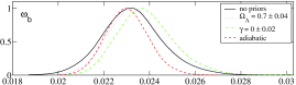
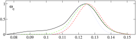
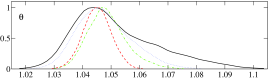
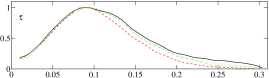
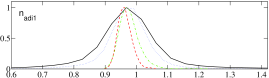
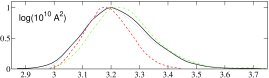
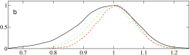
Figure 3: Marginalized likelihood functions for the standard cosmological parameters (i.e. those that exist in the adiabatic model). The solid (black) line is the likelihood in our 11-parameter model, the dashed (red) line is for the adiabatic model. Other line types show the effects of additional priors discussed in the text: dotted (blue) for Gaussian $\Omega_{\Lambda}=0.70\pm 0.04$, and dot-dashed (green) for Gaussian $\gamma=0.0\pm 0.02$.

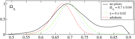
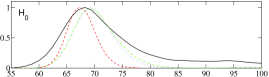
Figure 4: Marginalized likelihoods for two derived parameters, $\Omega_{\Lambda}$ and $H_{0}$. The line styles have the same meaning as in Fig. 3.

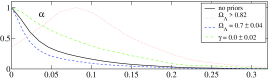
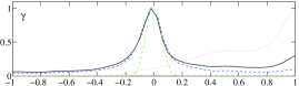
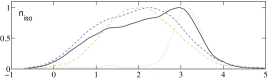
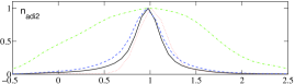
Figure 5: Marginalized likelihoods for the parameters related to the isocurvature mode and correlation. We show the $4$ remaining independent parameters, $\alpha$, $\gamma$, $n_{\rm{iso}}$, $n_{\rm{ad2}}$. The solid (black) line is the full likelihood, other line types show the effects of additional priors discussed in the text: dotted (red) for Gaussian $\Omega_{\Lambda}>0.82$, dashed (blue) for Gaussian $\Omega_{\Lambda}=0.70\pm 0.04$, and dot-dashed (green) for Gaussian $\gamma=0.0\pm 0.02$.

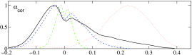
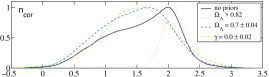
Figure 6: Marginalized likelihoods for the isocurvature-related derived parameters, $\alpha_{\mathrm{cor}}$ and $n_{\rm{cor}}$. The line styles have the same meaning as in Fig. 5.

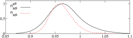
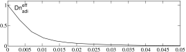
Figure 7: (a) Marginalized likelihoods for the effective adiabatic spectral index $n_{\rm{ad}}^{\mathrm{eff}}$ (solid line, black) compared to the spectral index of the pure adiabatic model $n_{\rm{ad}}$ (dashed line, red). (b) Marginalized likelihood for $dn_{\rm{ad}}^{\mathrm{eff}}/d\ln\bar{k}$ at the pivot scale $k_{0}=0.01\mbox{ Mpc}^{-1}$.

At our pivot scale we have $\bar{k}=1$ and the above expressions simplify to

$$\left.n_{\rm{ad}}^{\mathrm{eff}}\right|_{k=k_{0}}=(n_{\rm{ad1}}-1)(1-|\gamma|)+(n_{\rm{ad2}}-1)|\gamma|+1\,,$$ (25)

and

$$\left.\frac{dn_{\rm{ad}}^{\mathrm{eff}}(\bar{k})}{d\ln\bar{k}}\right|_{k=k_{0}}=\Big{(}n_{\rm{ad1}}-n_{\rm{ad2}}\Big{)}^{2}\Big{(}1-|\gamma|\Big{)}|\gamma|\,.$$ (26)

From Fig. 3 we observe that $n_{\rm{ad1}}$ is much more loosely constrained than the $n_{\rm{ad}}$ of the adiabatic model. The distribution for $n_{\rm{ad2}}$ becomes even wider than the one for $n_{\rm{ad1}}$, see Fig. 5. The reason is that the MCMC chains contain many models with $|\gamma|$ close to zero allowing $n_{\rm{ad2}}$ to take any value or $|\gamma|$ close to 1 allowing $n_{\rm{ad1}}$ to take any value. However, the effective adiabatic spectral index (25) becomes nearly as tightly constrained as the spectral index in pure adiabatic models. The 95% C.L. regions are $0.910<n_{\rm{ad}}^{\mathrm{eff}}<1.050$ with median $0.968$ and $0.923<n_{\rm{ad}}<1.013$ with median $0.961$, see also Fig. 7(a). Moreover, the data disfavor (positive) running of the adiabatic spectral index. For the 95% C.L. upper limit we obtain $dn_{\rm{ad}}^{\mathrm{eff}}/d\ln\bar{k}<0.03$ at $k_{0}=0.01$Mpc^-1, see Fig. 7(b). The largest $k$ in the data sets is about $k_{\mathrm{max}}\approx 0.15$Mpc^-1. So the maximum running from $k_{0}$ to $k_{\mathrm{max}}$ is approximately $\Delta n=0.03\times\ln(k_{\mathrm{max}}/k_{0})=0.08$. The quadrupole ($l=2$) corresponds to $k_{\mathrm{min}}\approx 1.4\times 10^{-4}$Mpc^-1 leading to $\Delta n=0.03\times\ln(k_{\mathrm{min}}/k_{0})=-0.12$.

IV.2 Small matter density models

In Fig. 3 the most obvious difference from the adiabatic model is the extension of the $\theta$ likelihood towards larger sound horizon angles and the $\omega_{c}$ likelihood towards smaller densities. These two features are related as can be seen in Fig. 8(a). The corresponding effect is seen in the two derived parameters, $\Omega_{\Lambda}$, $H_{0}$, closely related to $\theta$ and $\omega_{c}$, see Fig. 8(b). Compare to a simalar Fig. in Trotta et al. (2003).

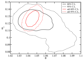
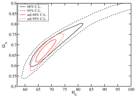
Figure 8: (a) 2-d marginalized likelihood for $\theta$ and $\omega_{c}$, showing that the large sound horizon angles $\theta$ are connected with low CDM densities $\omega_{c}$. We indicate the 68% (solid) and 95% (dashed) C.L. regions for our isocurvature model (black) and for the adiabatic model (red). (b) 2-d likelihood for the two derived parameters $H_{0}$ and $\Omega_{\Lambda}$ closely related to the independent parameters $\theta$ and $\omega_{c}$.

The 1-d likelihood for the derived parameter $\Omega_{\Lambda}$ show (Fig. 4) a second peak at $\Omega_{\Lambda}\sim 0.87$. (This feature is somewhat enhanced because the flat prior for our independent parameters actually leads to an increasing prior for the derived parameter $\Omega_{\Lambda}$, and larger values of $\Omega_{\Lambda}$ are cut off with our $h\leq 1$ constraint.)

Thus the possibility of an isocurvature contribution leads to larger $\Omega_{\Lambda}$ models becoming acceptable by the CMB and LSS data. According to Fig. 9 these models have a positive correlation between the adiabatic and isocurvature modes. Indeed, if we cut to the subset of “uncorrelated models”, $\gamma=0.0\pm 0.02$, the (large $\theta$, small $\omega_{c}$) feature disappears from the 1-d likelihoods.

In Figs. 5 and 6 we show the 1-d likelihoods of the isocurvature-related parameters separately for the large-$\Omega_{\Lambda}$ subset (dotted red lines) and with a $\gamma=0.0\pm 0.02$ prior that cuts the more correlated models off (dot-dashed green lines). We see clearly that the large-$\Omega_{\Lambda}$ models are associated with a positive correlation between the isocurvature and adiabatic modes.

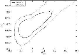
Figure 9: 2-d marginalized likelihood for $\alpha_{\mathrm{cor}}$ and $\Omega_{\Lambda}$, showing that the large $\Omega_{\Lambda}$ are connected with a positively correlated isocurvature contribution.

The angular and matter power spectra of the best-fit large-$\Omega_{\Lambda}$ model (from the subset $\Omega_{\Lambda}\geq 0.82$) are shown in Fig 10. This model has $\chi^{2}=1461.86$. Compared to the best-fit adiabatic model, the somewhat worse fit, $\Delta\chi^{2}=2.21$, is due to 1) a worse fit to the SDSS data ($\Delta\chi^{2}=1.83$) and 2) a worse fit to the Sachs-Wolfe region ($2\leq l\leq 21$) of the WMAP TT data ($\Delta\chi^{2}=2.51$). The latter is due to the increased late ISW effect caused by the larger $\Omega_{\Lambda}$. This model fits the rest of the CMB data better than the adiabatic model.

The reason the larger sound horizon angles (which shift the acoustic peaks left, i.e., towards smaller $l$) are accepted is the correlation contribution $C^{\mathrm{cor}}_{l}$, whose acoustic peaks are at somewhat larger $l$ than the adiabatic ones, and thus adding it appears as a shifting of the peaks to the right (i.e., towards larger $l$). An uncorrelated isocurvature contribution cannot do the same trick, since the isocurvature acoustic peaks are too much to the right for adding them to appear as a shift in peak position. The distribution of the isocurvature spectral index is concentrated at the upper end of the allowed range for $n_{\rm{iso}}$ in these $\Omega_{\Lambda}>0.82$ models, see again Figs. 5 and 6. This is required for the correlation contribution to maintain roughly the same relative power through the acoustic peak region.

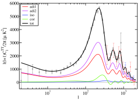
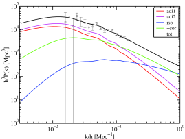
Figure 10: (a) The TT spectrum for the best-fit large $\Omega_{\Lambda}$ ($\Omega_{\Lambda}>0.82)$ model, showing how the correlation part contributes towards shifting the acoustic peaks to the right. This model has $\omega_{b}=0.0221$, $\omega_{c}=0.100$, $\theta=1.082$, $\tau=0.177$, $b=0.796$, $\ln(10^{10}A^{2})=3.24$, $n_{\rm{ad1}}=0.949$, $\alpha=0.108$, $n_{\rm{iso}}=3.11$, $\gamma=0.57$, $n_{\rm{ad2}}=1.043$. The correlated adiabatic component (“ad2”, magenta) dominates over the uncorrelated adiabatic component (“ad1”, red). The other curves are the correlation component (“cor”, green) and isocurvature component (“iso”, blue). The total angular power (“tot”, black) is a sum of these components. (b) The matter power spectrum, showing how the correlation contribution changes its shape.

Because of this large spectral index, especially the correlation contribution also changes the shape of the matter power spectrum, see Fig. 10(b). This allows for a smaller “shape parameter” $\Omega_{m}h$ to fit the SDSS data, than the SDSS result $\Omega_{m}h=0.21\pm 0.03$ for adiabatic models. In the adiabatic model, large values of $\Omega_{\Lambda}$ and $h$ would be allowed by either the CMB or the LSS data alone, but not by the combined data sets, because either data set allows a narrow region (the “vanilla banana” in Fig. 5 of Tegmark et al. (2004b)) in the $(\Omega_{\Lambda},h)$ plane, but these regions have somewhat different orientations. The correlation contribution makes both regions wider, in such a way that their overlap is extended to higher $h$ and smaller $\Omega_{m}$ (larger $\Omega_{\Lambda}$), or in terms of our independent parameters, towards smaller $\omega_{c}$. In fact, even $h>1.0$, with $\Omega_{m}<0.1$ (or $\Omega_{\Lambda}>0.9$) would be allowed, but our $h\leq 1.0$ prior cuts them off. These models also favor smaller bias parameters $b$ and baryon densities $\omega_{b}$.

One might expect the above to work in the other direction too, negative correlation allowing models with a smaller $\theta$, $\Omega_{\Lambda}$, $h$, and a larger $\omega_{c}$, but apparently some other feature in the data prevents the larger $\omega_{c}$ required.

The large values of $\Omega_{\Lambda}$ are ruled out by the high-$z$ Type Ia Supernovae redshift-magnitude (SNIa) dataRiess et al. (2004). Therefore the large-$\Omega_{\Lambda}$ feature was not seen in Beltran et al. (2004). We did not use the SNIa data; but to study the effect of a SNIa constraint we simulated it by importance weighting our MCMC chains with a Gaussian $\Omega_{\Lambda}=0.70\pm 0.04$ distribution. We show the 1-d likelihoods both with and without this extra prior in Figs. 3–6. The effect of this SNIa constraint cutting the (large $\theta$, small $\omega_{c}$) models off is clearly seen in them.

IV.3 Baryon density and Hubble parameter

In pure adiabatic models the baryon density is practically determined by the heights of the first and second acoustic peaks (and the valley between them). An isocurvature contribution modifies these heights and thus one expects looser constraint for $\omega_{b}$ in mixed adiabatic and isocurvature models. However, our constraints ($0.0220<\omega_{b}<0.0246$ at 68% C.L., $0.0207<\omega_{b}<0.0263$ at 95% C.L., median $0.0232$) are very close to the adiabatic model ($0.0221<\omega_{b}<0.0240$ at 68% C.L., $0.0213<\omega_{b}<0.0250$ at 95% C.L., median $0.0230$). Moreover, we have checked that the isocurvature amplitude ($\alpha$) dependence of the constraints for $\omega_{b}$ is very weak within the allowed range $\alpha<0.18$.

As can be seen in Fig. 3 the median of $\omega_{b}$ shifts only marginally towards larger values regardless of the (extra) priors chosen. Our result is consistent with Beltran et al. (2004) where the 1-d likelihoods for the adiabatic reference model and for the correlated CDM isocurvature model were practically indistinguishable. (The neutrino isocurvature modes shifted $\omega_{b}$ towards smaller values unlike in some other models to be discussed below.)

Both our result and the likelihood for $\omega_{b}$ in Beltran et al. (2004) differ from Moodley et al. (2004) where the median shifted significantly towards larger values ($0.023<\omega_{b}<0.029$ at 68% C.L., median $0.026$). In their model the adiabatic, CDM isocurvature and correlation spectral indices were kept equal, i.e. they had only one free spectral index. Both Beltran et al. (2004) and Moodley et al. (2004) used CMB and LSS data sets very similar to those used by us. On the other hand, in Ferrer et al. (2004) the curvaton decay calculation (see e.g. Gupta et al. (2004)) was extended to the case when the curvaton does not necessarily behave like dust. The resulting correlated CDM isocurvature perturbations from the mixed inflaton-curvaton decay (or e.g. from double-inflation which produce primordial power spectrum of similar type) were considered in the light of WMAP data alone. Then $\omega_{b}$ got even larger values. The 68% C.L. region obtained in Ferrer et al. (2004) was $0.027<\omega_{b}<0.042$ with median $0.032$. (The best-fit model had $\omega_{b}=0.041$.) Although, the form of the primordial power spectrum in Ferrer et al. (2004, 2005) looks quite similar to ours, the important difference is that the adiabatic and isocurvature components have equal spectral indices there. Note however, that as the curvature and entropy perturbations are both a sum of two components the model has two independent spectral indices insted of just one of Moodley et al. (2004). In Bucher et al. (2004) a model with equal spectral indices for adiabatic, CDM isocurvature and neutrino isocurvature modes yielded also very large $\omega_{b}\sim 0.04$. The CMB data alone led to a bit larger $\omega_{b}$ than CMB and LSS data together.

Three years ago Trotta, Riazuelo, and Durrer demonstrated in Trotta et al. (2001) that allowing for “general isocurvature modes” (adiabatic, CDM isocurvature and neutrino isocurvature with equal spectral indices in their study) prevented one from obtaining an upper bound for $\omega_{b}$ from that day’s CMB data (COBE Smoot et al. (1992); Bennett et al. (1994); Tegmark and Zaldarriaga (2000) and Boomerang Netterfield et al. (2002)). In Trotta et al. (2001) most of the new freedom for $\omega_{b}$ was explained to come from the neutrino isocurvature density mode which can adjust the height of the second acoustic peak more than other isocurvature modes. Hence, one would expect more freedom for $\omega_{b}$ when allowing also for a neutrino isocurvature density mode instead of just a CDM isocurvature mode (or a neutrino isocurvature velocity mode). However, one can not see this effect in Beltran et al. (2004) where the median of $\omega_{b}$ was shifted a bit towards smaller values (compared to other cases) and the width of the 1-d distribution remained small. While part of the different effect of the neutrino isocurvature density mode in Trotta et al. (2001) and Beltran et al. (2004) could result from the different data sets used (the former used CMB only, the latter used precision CMB and LSS), we think that the fundamental explanation resides in spectral indices. The same applies to other isocurvature modes.

To be explicit, our model and the model in Beltran et al. (2004) (both have three independent spectral indices) yield very little difference to the adiabatic case whereas models studied in Moodley et al. (2004); Bucher et al. (2004); Ferrer et al. (2004); Trotta et al. (2001) (all have “$n_{\rm{ad}}=n_{\rm{iso}}$”) lead to larger medians and wider distributions for $\omega_{b}$. While we have not studied in detail the reason for this difference, we discuss one possibility. The CMB data forces the dominant adiabatic spectrum close to scale invariance ($n_{\rm{ad}}\sim 1$). When the spectral indices are kept equal (“$n_{\rm{ad}}=n_{\rm{iso}}$”) the isocurvature component also acquires the same spectral index. The multipole dependence of the isocurvature contribution to the CMB spectrum can now be seen easily from Fig. 2(c). Isocurvature and correlation modify more the low multipole end of the spectrum than high multipoles. There is a large difference in the power coming from non-adiabatic contributions to the Sachs-Wolfe plateau ($l\lesssim 21$) and to the first or second acoustic peak. Hence, the acoustic peak structure is distorted significantly leading to a need/possibility to adjust it by $\omega_{b}$. However, if the isocurvature spectral index is a free parameter it acquires a value that leads to a small isocurvature contribution on all scales. This happens with $n_{\rm{iso}}\sim 3$ as will be demonstrated in Fig. 13. With this large $n_{\rm{iso}}$ the isocurvature contribution to the $C_{l}$ and to the matter power can remain, e.g., at some 3.5% level (for our median $\alpha=0.035$) on all scales. Then the different peak structure of the isocurvature compared to the adiabatic one represents only a marginal distortion from the pure adiabatic case. This explains why we and Beltran et al. (2004) end up with the “adiabatic value” for $\omega_{b}$.

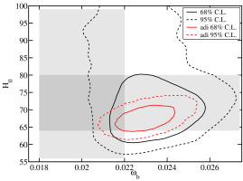
Figure 11: The 68% (solid) and 95% (dashed) C.L. regions in the $(\omega_{b},H_{0})$ plane for our isocurvature model (black) and for the adiabatic model (red). The rectangular gray boxes represent a BBN constraint $\omega_{b}=0.020\pm 0.002$ Burles et al. (2001) and the HST constraint $H_{0}=(72\pm 8)$ km/s/Mpc Freedman et al. (2001).

The isocurvature effect on the determination of the Hubble parameter in our model is more dramatic. Without extra priors we do not obtain an upper bound for $h$ (within the analyzed range $0.4<h<1.0$), see Fig. 4 and the discussion of the previous subsection. (However, with a different choice of the pivot scale we would miss the small matter density models and hence obtain an upper bound for $h$. We will discuss this in detail in Sec. VI.) Applying the SNIa result $\Omega_{\Lambda}=0.70\pm 0.04$ to get rid of the large $h$ values we get a 95% C.L. region $0.64<h<0.77$.

In Fig. 11 we compare our model with the pure adiabatic model by showing the C.L. contours in $(\omega_{b},H_{0})$ plane. We indicate also the 95% C.L. result $\omega_{b}=0.020\pm 0.002$ from a big bang nucleosynthesis (BBN) calculation Burles et al. (2001) and the Hubble space telescope key project result $h=0.72\pm 0.08$ Freedman et al. (2001). The 95% region (or even the 68% region) of our model certainly accommodates the HST result, but is only marginally consistent with the BBN value of $\omega_{b}$ from Burles et al. (2001). Actually, the same is true for the adiabatic model. On the other hand, concordance is achieved with another BBN value $\omega_{b}=0.022\pm 0.002$ from Hagiwara et al. (2002).

For comparison, the similar contours opened up towards the upper right corner of $(\omega_{b},h)$ plane in Trotta et al. (2001). Moreover, the only “excluded region” was “an upper left corner” of their $(\omega_{b},h)$ plane where the BBN and HST regions intersected in their Fig. Again we stress that different data sets were used in Trotta et al. (2001), also neutrino isocurvature modes were allowed and there was only one spectral index. In any case, the considerations in this subsection demonstrate that even within “isocurvature models” the initial assumptions, e.g. the shape assumed for the primordial spectrum, affect considerably the end results.

IV.4 Isocurvature parameters

We now turn to the parameters related to isocurvature perturbations. The 1-d likelihoods for the 4 independent parameters, the isocurvature fraction $\alpha$, the isocurvature spectral index $n_{\rm{iso}}$, the adiabatic correlated fraction $\gamma$, and the spectral index $n_{\rm{ad2}}$, are shown in Fig. 5, and the two derived parameters, the correlation fraction

$$\alpha_{\mathrm{cor}}\equiv\mathrm{sign}(\gamma)\sqrt{\alpha(1-\alpha)|\gamma|}$$ (27)

and the correlation spectral index

$$n_{\rm{cor}}\equiv\frac{n_{\rm{ad2}}+n_{\rm{iso}}}{2}\,.$$ (28)

in Fig. 6.

We obtain an upper limit (95% C.L.) to the isocurvature fraction

$$\alpha<0.18\,.$$ (29)

One should be careful about the meaning of this. First, $\alpha$ is defined as the isocurvature fraction at our pivot scale $k_{0}=0.01\mbox{Mpc}^{-1}$. Models with a small isocurvature fraction at this scale may have a large isocurvature fraction at some other scale, depending on how the spectral indices for the adiabatic and isocurvature fractions differ from each other. Second, since $\alpha$ is defined in terms of the primordial curvature and entropy perturbations, it does not give directly the relative isocurvature contribution to $C_{l}$, but that depends also on the shapes of the component spectra $\hat{C}^{\mathrm{ad1}}_{l}$, $\hat{C}^{\mathrm{ad2}}_{l}$, $\hat{C}^{\mathrm{cor}}_{l}$, and $\hat{C}^{\mathrm{iso}}_{l}$, (i.e., on the transfer functions) which depend on the other cosmological parameters, and are typically such that the isocurvature contribution to the total $C_{l}$ and $P(k)$ is smaller than $\alpha$. Thus the limit to an isocurvature signal in the data is actually tighter than would appear from Eq. (29). (See Sec. V.) Third, because of the presence of poorly constrained parameters, $n_{\rm{ad2}}$ and $n_{\mathrm{iso}}$ in the case of small $\gamma$ or $\alpha$, the likelihood functions, and thus upper limits, are sensitive to the priors implied by the choice of parametrization. We discuss this last point in Sec. VI. Similar caveats apply to the other isocurvature related parameters.

For the “uncorrelated” subset, $\gamma=0.0\pm 0.02$ the formal upper limit is larger

$$\alpha<0.22\,.$$ (30)

The limit for correlated models is tighter, since the correlation contribution to the data tends to be larger than the isocurvature contribution, due to the transfer functions (see Figs. 1 and 2), and since $|\alpha_{\mathrm{cor}}|\equiv\sqrt{\alpha(1-\alpha)|\gamma|}>\alpha$ for small $\alpha$ and moderate $\gamma$.

The isocurvature spectral index has a fairly wide distribution covering the range $0<n_{\rm{iso}}<4$. The median value is $n_{\rm{iso}}=2.252$. The distribution is skew, so that the largest marginalized likelihood is at somewhat larger values, $n_{\rm{iso}}\sim 3.0$. This peak at $n_{\rm{iso}}$ comes from the large-$\Omega_{\Lambda}$-models discussed in Sec. IV.2. Otherwise, values $1<n_{\rm{iso}}<3$ are preferred. Fig. 12 shows the 2-d likelihood for $\alpha$ and $n_{\rm{iso}}$.

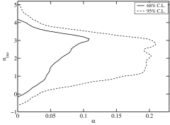
Figure 12: 2-d marginalized likelihood for $\alpha$ and $n_{\rm{iso}}$.

There are basically two reasons why the data selects this range for $n_{\rm{iso}}$. Disregarding the peak structure in the $C_{l}$ spectrum, the overall distribution of power in the data over different scales is such that for the adiabatic models it favors a scale-independent $n_{\rm{ad}}\sim 1$ primordial spectrum. For the isocurvature modes the $C_{l}$ transfer function falls more steeply with $k$ (see Figs. 1 and 2.) Thus, for the isocurvature contribution not to disturb this overall distribution of power, it needs a larger spectral index. The other reason is in the more detailed shape of the data. The CMB data clearly does not like the isocurvature contribution, since it has the wrong peak structure. Too small (large) $n_{\rm{iso}}$ would cause it to show up for small (large) $l$, even for small $\alpha$. With $k_{0}$ in the middle of the data sets, this keeps $0<n_{\rm{iso}}<4$.

In Fig. 13 we show the unit-amplitude component $\hat{C}_{l}$ spectra, for $n_{\rm{ad}}$ still at $1$, but $n_{\rm{iso}}$ at the median value, $n_{\rm{iso}}=2.252$. Now the effective slope of the adiabatic and isocurvature contributions is roughly the same, so that the isocurvature contribution is kept low everywhere with moderately small $\alpha$.

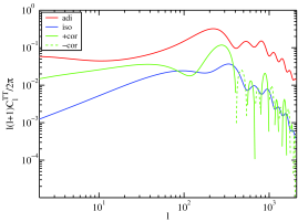
Figure 13: Like Fig. 2(c), but now with $n_{\rm{iso}}=2.252$.

IV.5 Correlation Parameters

Zero correlation, $\gamma\approx 0$, is favored over any other particular value for the correlation. However, 61% of the models have $|\gamma|\geq 0.1$ (Fig. 5). Positive correlations are favored over negative ones.

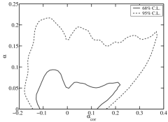
Figure 14: 2-d marginalized likelihood for $\alpha_{\mathrm{cor}}$ and $\alpha$.

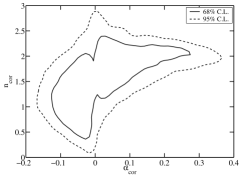
Figure 15: 2-d marginalized likelihood for $\alpha_{\mathrm{cor}}$ and $n_{\rm{cor}}$.

A strong correlation $\gamma$ between the adiabatic and isocurvature perturbations however has little effect on the data, if the isocurvature perturbations, with which the adiabatic perturbations are correlated, are negligibly small. The signature in the data is better measured by the derived parameter $\alpha_{\mathrm{cor}}$ (which is restricted between $\pm\sqrt{\alpha(1-\alpha)}$ by definition). We see that the 1-d likelihood of $\alpha_{\mathrm{cor}}$ is skew (Fig. 6); the preference for positive correlations that we saw in $\gamma$ appears here as a long tail towards large $\alpha_{\mathrm{cor}}$. If we add the Gaussian prior $\Omega_{\Lambda}=0.70\pm 0.04$ to represent SNIa constraints, this tail goes away, and the 1d likelihood becomes rather symmetric. Thus the preference for positive correlations is due to the large-$\Omega_{\Lambda}$ models discussed in Sec. IV.2. The dip at $\alpha_{\mathrm{cor}}=0$ in Figs. 6, 14, and 15 does not indicate that uncorrelated models would be unfavored by the data; rather it comes because flat priors for $\alpha$ and $\gamma$ lead to a prior for $\alpha_{\mathrm{cor}}$ which is small for small $\alpha_{\mathrm{cor}}$. Fig. 14 shows the 2-d likelihood of $\alpha$ and $\alpha_{\mathrm{cor}}$.

In Fig. 15 we show the 2-d likelihood of $\alpha_{\mathrm{cor}}$ and $n_{\rm{cor}}$. It shows that positive correlations are connected with larger spectral indices $n_{\rm{cor}}$ than negative correlations. This feature remains also after applying the $\Omega_{\Lambda}=0.70\pm 0.04$ prior, although the largest $\alpha_{\mathrm{cor}}$ values are cut off. For large $|\gamma|$ we have $n_{\rm{ad2}}\approx 1$, and thus

$$n_{\rm{cor}}\equiv\frac{n_{\rm{ad2}}+n_{\rm{iso}}}{2}\approx\frac{1+n_{\rm{iso}}}{2}\,.$$ (31)

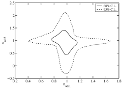
Figure 16: 2-d marginalized likelihood for $n_{\rm{ad1}}$ and $n_{\rm{ad2}}$.

The reason negative correlations are favored with smaller $n_{\rm{cor}}$ is that then there is a significant isocurvature and correlation contribution to the Sachs-Wolfe region of the TT spectrum, and the negative correlation now subtracts from it, helping to fit the lowest $l$ WMAP data points which lie below the adiabatic spectra (see Fig. 17).

For larger $n_{\rm{cor}}$ the correlation contribution is insignificant in the SW region, but becomes important in the region of acoustic peaks and for the matter power spectrum. Positive correlations are now favored for the reasons discussed in Sec. IV.2. This effect remains after adding the Gaussian prior $\Omega_{\Lambda}=0.70\pm 0.04$, in part since this SNIa result favors somewhat larger $\Omega_{\Lambda}$ than the CMB+SDSS data applied to adiabatic models.

Whenever one adiabatic component has negligible amplitude, the corresponding spectral index (i.e., $n_{\rm{ad2}}$ for $\gamma\approx 0$, and $n_{\rm{ad1}}$ for $|\gamma|\sim 1$) becomes unconstrained (see Fig. 16), otherwise it is tightly constrained to be near $1$. When both components are significant, there is a small anticorrelation between $n_{\rm{ad1}}$ and $n_{\rm{ad2}}$ Valiviita and Muhonen (2003), as a red tilt in one of them can compensate for a blue tilt in the other one, making the sum closer to scale-invariant (as preferred by the data). This effect however introduces a positive $dn/d\ln k$ in the combined spectrum (Sec. IV.1), which the data does not like, especially with the inclusion of LSS data, and therefore the anticorrelation effect is now more limited than in Valiviita and Muhonen (2003).

In Fig. 17 we show the spectra for our best-fit model. This is an example of a low-$n_{\rm{iso}}$, negative-correlation model, where the correlation contribution subtracts from the Sachs-Wolfe region in the $C_{l}$. This model has $\omega_{b}=0.0227$, $\omega_{c}=0.129$, $\theta=1.043$, $\tau=0.144$, $b=0.962$, $\ln(10^{10}A^{2})=3.30$, $n_{\rm{ad1}}=0.988$, $\alpha=0.00197$, $n_{\rm{iso}}=0.388$, $\gamma=-0.67$, $n_{\rm{ad2}}=0.926$, and $\chi^{2}=1459.29$.

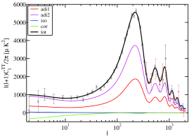
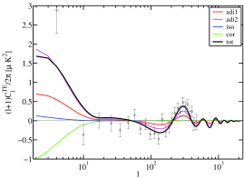
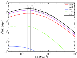
Figure 17: The CMB and matter power spectra for our best-fit model. The correlated adiabatic component (“ad2”, magenta) dominates over the uncorrelated adiabatic component (“ad1”, red) and the negative correlation subtracts from the Sachs-Wolfe region of the CMB spectrum.

IV.6 Models with Very Large Isocurvature Spectral Index

We set a very wide allowed range for the isocurvature spectral index. While most of the good models had $n_{\rm{iso}}$ in the range $0$ to $4$, one of our MCMC chains found an apparently very good region where $n_{\rm{iso}}$ was between $5$ and $6$. In fact the highest likelihood ($\chi^{2}=1459.20$) was obtained in this region. We did not have enough statistics to assess correctly the relative importance of this disjoint good-likelihood region in the parameter space. We discard this region for reasons explained below. Thus we have not included this chain in our full analysis. (And therefore we do not take our best-fit model from it.) In fact, these models are obviously nonsense, and we discuss them just as a warning.

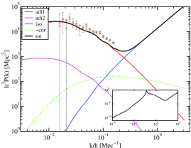
Figure 18: The matter power spectrum of a model with $n_{\rm{iso}}$=5.69, which has $\chi^{2}=1459.20$. The inset shows the SDSS window function for the 16th, i.e. second from right, data point. The red markers ($\ast$) indicate the values (theoretical matter power spectrum convolved with the window function) to be compared to the data points, showing that the fit ($\chi^{2}$) obtained this way is very good, although the power spectrum seems to lie below the data. The problem with this kind of matter power is that the window function picks most of the “power” from the non-linear regime. Moreover, we have calculated the matter power up to $k/h\sim 3$Mpc^-1 only. Had we calculated further, the rapidly rising power at large $k$ would have caused the red markers ($\ast$) to move up leading to worse $\chi^{2}$ for this model.

These models necessarily have a very small $\alpha$; because of the large $n_{\rm{iso}}$ the isocurvature contribution is steeply rising, and only becomes noticeable at the smallest scales of our data set. At scales smaller than included in our data set, the isocurvature contribution then becomes dominant, and $P(k)$ rises rapidly.

Thus for most of the data set, these models are essentially equal to the adiabatic model. The improvement over the adiabatic model is then in the ”other CMB” and ”SDSS” data which cover the smallest scales. The fit to the SDSS data is however obtained in a rather unnatural way. Because the SDSS window functions, that describe how the data points relate to the underlying power spectrum, extend to much smaller scales (larger $k$) than the nominal $k$ values of the data points, for these models they pick up most of the contribution at these very small scales (see Fig. 18). Since the perturbations are non-linear at these scales, our use of a linear power spectrum does not give correct results. (We also suspect that the SDSS window functions were not really meant to be used for this kind of spectra.) Anyway, these models would be ruled out if some smaller scale constraints were added.

Because our pivot scale is far enough to the left from the right (small-scale) end of our data set, these models are forced to have a rather small $\alpha$, which makes the measure of this region of parameter space rather small. If a smaller pivot scale (larger $k_{0}$) is used, it becomes more likely for the MCMC chains to end up in this questionable region (Sec.VI).

V Non-adiabatic contribution to the observed spectra

So far we have constrained the non-adiabatic contribution to the primordial spectrum in terms of $\alpha$ and $\alpha_{\mathrm{cor}}$ (or $\gamma$). Although the isocurvature component can be as large as 18% of the total primordial power at our pivot scale $k_{0}$, its role in the observed $C_{l}$ (or matter power) spectrum is less significant. This comes because of different behavior of adiabatic and isocurvature transfer functions as discussed in Secs. II and IV.4. Moreover, the non-scale-invariant spectral index complicates drawing conclusions for the observed $C_{l}^{\mathrm{iso}}$ and $C_{l}^{\mathrm{cor}}$ from $\alpha$ and $\alpha_{\mathrm{cor}}$, respectively. Thus we devote this section to finding limits for non-adiabatic contributions to the observed spectra.

We define a relative non-adiabatic contribution to $C_{l}^{\mathrm{TT}}$ by

$$\alpha_{l}=\frac{C_{l}^{\mathrm{TTiso}}+C_{l}^{\mathrm{TTcor}}}{C_{l}^{\mathrm{TT}}}\,,$$ (32)

where $C_{l}^{\mathrm{TT}}=C_{l}^{\mathrm{TTad1}}+C_{l}^{\mathrm{TTad2}}+C_{l}^{\mathrm{TTiso}}+C_{l}^{\mathrm{TTcor}}$. When creating MCMC chains we saved this quantity for $l=2$, $140$, $200$, and $700$ for each accepted step. By similar manner we define a non-adiabatic contribution to the matter power at $k=k_{i}$

$$\alpha_{mi}=\frac{{P}^{\mathrm{iso}}(k_{i})+{P}^{\mathrm{cor}}(k_{i})}{{P}^{(}k_{i})}\,.$$ (33)

We saved this around the first SDSS data point $k_{1}/h=0.0154$ Mpc^-1 and at the last data point $k_{17}/h=0.154$ Mpc^-1.

The range of possible values for $\alpha_{l}$ and $\alpha_{mi}$ is $[-\infty,1]$. For example, $\alpha_{l}$ gets negative values whenever $C_{l}^{\mathrm{cor}}<-C_{l}^{\mathrm{iso}}$. In the extreme case that $C_{l}^{\mathrm{iso}}=C_{l}^{\mathrm{ad2}}$ and $C_{l}^{\mathrm{cor}}=-2C_{l}^{\mathrm{iso}}$ the denominator approaches zero in the absence of $C_{l}^{\mathrm{ad1}}$. On the other hand, the maximum value $1$ is obtained with $C_{l}^{\mathrm{cor}}=C_{l}^{\mathrm{ad2}}=C_{l}^{\mathrm{ad1}}=0$.

Recall that the $C_{l}^{\mathrm{TT}}$s are related to the variance of the CMB temperature perturbation by

$${\textstyle\left\langle\left(\frac{\delta T}{T}\right)^{2}\right\rangle}=\frac{1}{4\pi}\sum_{l=0}^{\infty}(2l+1)C^{TT}_{l}\,.$$ (34)

We have calculated the $C_{l}$ for $l=2$–$2100$. In all well-fitting models

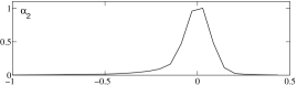
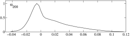
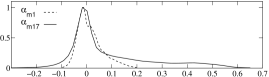
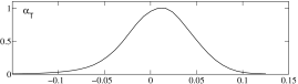
Figure 19: Marginalized likelihoods of non-adiabatic contributions to the observed spectra in our 11 parameter model.

the power at $l=2100$ is negligible due to diffusion damping. These considerations lead us to one more measure of the non-adiabatic contribution

$$\alpha_{T} = \frac{\langle(\delta T^{\mathrm{non-ad}})^{2}\rangle}{\langle(\delta T^{\mathrm{total}})^{2}\rangle}$$ (35)

$$= \frac{\sum_{l=2}^{2100}\left(2l+1\right)\left(C_{l}^{\mathrm{TTiso}}+C_{l}^{\mathrm{TTcor}}\right)}{\sum_{l=2}^{2100}\left(2l+1\right)C_{l}^{\mathrm{TT}}}\,.$$

Correlated models. In Fig. 19 we plot the marginalized 1-d likelihoods for $\alpha_{2}$, $\alpha_{200}$, $\alpha_{m1}$, $\alpha_{m17}$, and $\alpha_{T}$. At the quadrupole ($l=2$) a long tail of $\alpha_{2}$ towards negative non-adiabatic contribution appears, since the measured quadrupole is rather low compared to typical pure adiabatic models. The 95% C.L. region spans an interval $-0.46<\alpha_{2}<0.10$. Around the first acoustic peak the non-adiabatic contribution is much more constrained, $-0.024<\alpha_{200}<0.079$, and at $l=700$ the allowed contribution becomes even smaller, $-0.011<\alpha_{700}<0.026$. In the matter power, the limits are $-0.06<\alpha_{m1}<0.14$ and $-0.11<\alpha_{m17}<0.51$. The latter, quite large values come because we do not use any data from larger $k$. So the spectrum is practically unconstrained after $k_{17}$. (Recall also our warning example in Figure 18.) The likelihood for the total non-adiabatic temperature perturbation is quite symmetric with the median at $\alpha_{T}=0.009$ and a 95% C.L. interval $-0.075<\alpha_{T}<0.075$. Hence, we conclude that the non-adiabatic contribution to the observed temperature perturbation is less than 7.5%.

Uncorrelated models. Four years ago we Enqvist et al. (2000) found upper limits for an uncorrelated CDM isocurvature contribution using the first data releases of Boomerang de Bernardis et al. (2000) and Maxima Balbi et al. (2000) together with COBE data Tegmark and Zaldarriaga (2000). The 95% C.L. limits were $\alpha_{2}<0.56$ (called $\alpha$ in Enqvist et al. (2000)) and $\alpha_{200}<0.13$. Let us update these numbers to reflect the dramatically increased accuracy of the data. We approximate uncorrelated models by applying a Gaussian prior $\gamma=0.00\pm 0.02$ when analyzing the chains.

Figure 20: Marginalized likelihoods of non-adiabatic contributions to the observed spectra in “uncorrelated models” ($\gamma=0.0\pm 0.02$).

Since the data does not favor correlation (see Figure 5), the sampling of models with small $|\gamma|$ is very good. For uncorrelated models the correlation component is missing from definitions (32), (33), and (35). Then the range for $\alpha_{l}$, $\alpha_{mi}$ and $\alpha_{T}$ is $[0,1]$. 1-d likelihoods are given in Fig. 20. The 95% C.L. limits are $\alpha_{2}<0.085$ and $\alpha_{200}<0.023$. So, the allowed isocurvature contribution in the uncorrelated case has dropped to about one sixth part of the limits obtained four years ago. Finally, the allowed total non-adiabatic contribution ($\alpha_{T}$) to the observed temperature perturbation signal becomes less than 4.3%.

VI Effect of Choice of Pivot Scale

When the modes have different spectral indices, the relative amplitude parameters $\alpha$ and $\gamma$ become dependent on the choice of pivot scale $k_{0}$. In the literature, different pivot scales have been used, e.g., $k_{0}=0.002\mbox{ Mpc}^{-1}$ and $k_{0}=0.05\mbox{ Mpc}^{-1}$, whereas we have chosen an intermediate value $k_{0}=0.01\mbox{ Mpc}^{-1}$.

One can convert the results obtained using one pivot scale $k_{0}$ to what one would get with another pivot scale $\tilde{k}_{0}$, by using the parameter transformation

$$\tilde{\alpha}=\frac{\alpha\hat{k}^{n_{\rm{iso}}-1}}{(1-\alpha)(1-|\gamma|)\hat{k}^{n_{\rm{ad1}}-1}+(1-\alpha)|\gamma|\hat{k}^{n_{\rm{ad2}}-1}+\alpha\hat{k}^{n_{\rm{iso}}-1}}$$ (36)

$$\tilde{\gamma}=\frac{\gamma\hat{k}^{n_{\rm{ad2}}-1}}{(1-|\gamma|)\hat{k}^{n_{\rm{ad1}}-1}+|\gamma|\hat{k}^{n_{\rm{ad2}}-1}}$$ (37)

$$\tilde{A}^{2}=A^{2}\left[(1-\alpha)(1-|\gamma|)\hat{k}^{n_{\rm{ad1}}-1}+(1-\alpha)|\gamma|\hat{k}^{n_{\rm{ad2}}-1}+\alpha\hat{k}^{n_{\rm{iso}}-1}\right]\,,$$ (38)

where $\hat{k}\equiv\tilde{k}_{0}/k_{0}$, and weighting the likelihoods with the Jacobian determinant of this parameter transformation,

$$J=\frac{\hat{k}^{n_{\rm{ad1}}-1}\hat{k}^{n_{\rm{ad2}}-1}\hat{k}^{n_{\rm{iso}}-1}}{\left[(1-|\gamma|)\hat{k}^{n_{\rm{ad1}}-1}+|\gamma|\hat{k}^{n_{\rm{ad2}}-1}\right]\left[(1-\alpha)(1-|\gamma|)\hat{k}^{n_{\rm{ad1}}-1}+(1-\alpha)|\gamma|\hat{k}^{n_{\rm{ad2}}-1}+\alpha\hat{k}^{n_{\rm{iso}}-1}\right]^{2}}\,.$$ (39)

This weighting gives the effect of changing from flat priors for $\alpha$, $\gamma$, and $\ln A$ to flat priors for $\tilde{\alpha}$, $\tilde{\gamma}$ and $\ln\tilde{A}$.

Typically we have $n_{\rm{ad1}}\approx n_{\rm{ad2}}\approx 1$, so that

$$\tilde{\alpha} \approx \frac{\alpha\hat{k}^{n_{\rm{iso}}-1}}{1-\alpha+\alpha\hat{k}^{n_{\rm{iso}}-1}}\sim\alpha\hat{k}^{n_{\rm{iso}}-1}$$ (40)

$$\tilde{\gamma} \approx \gamma$$ (41)

$$\tilde{A}^{2} \approx A^{2}\left(1-\alpha+\alpha\hat{k}^{n_{\rm{iso}}-1}\right)\sim A^{2}$$ (42)

and

$$J\approx\frac{\hat{k}^{n_{\rm{iso}}-1}}{\left(1-\alpha+\alpha\hat{k}^{n_{\rm{iso}}-1}\right)^{2}}\sim\hat{k}^{n_{\rm{iso}}-1}\,,$$ (43)

where the “$\sim$” are for small $\alpha$. Thus, if $\tilde{k}_{0}>k_{0}$, the likelihood of models with large $n_{\rm{iso}}$ is increased and that of small $n_{\rm{iso}}$ is decreased and the opposite holds if $\tilde{k}_{0}>k_{0}$.

To study the effect of varying $k_{0}$, we both (1) applied the above transformation to our results from our main run and (2) did shorter MCMC runs (8 chains) using $k_{0}=0.002\mbox{ Mpc}^{-1}$ and $k_{0}=0.05\mbox{ Mpc}^{-1}$. Both methods should give the same result if the MCMC runs have sufficient statistics. In practice, the results were close to each other for $k_{0}=0.002\mbox{ Mpc}^{-1}$, but for $k_{0}=0.05\mbox{ Mpc}^{-1}$, our original run had insufficient sampling at large $n_{\rm{iso}}$, for the reparameterization to give meaningful results. We show in Fig. 21 the resulting marginalized likelihoods for the (primary) parameters most affected. For $k_{0}=0.002\mbox{ Mpc}^{-1}$ the result shown is by method (1), but for $k_{0}=0.05\mbox{ Mpc}^{-1}$ by method (2), since it had better statistics. However, these results should only be taken as indicative, especially for $k_{0}=0.05\mbox{ Mpc}^{-1}$ as the statistics was not nearly as good as in our main case, $k_{0}=0.01\mbox{ Mpc}^{-1}$.

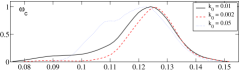
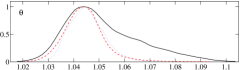
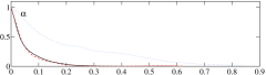
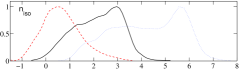
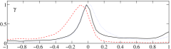
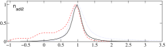
Figure 21: 1-dimensional likelihoods for $\omega_{c}$, $\theta$, $\alpha$, $n_{\rm{iso}}$, $\gamma$, and $n_{\rm{ad2}}$, using three different pivot scales, $k_{0}=0.002\mbox{Mpc}^{-1}$ (dashed, red), $k_{0}=0.01\mbox{Mpc}^{-1}$ (solid, black), and $k_{0}=0.05\mbox{Mpc}^{-1}$ (dotted, blue).

The 1-d likelihoods of $\omega_{b}$, $\tau$, $b$, and $n_{\rm{ad1}}$ did not change significantly. Thus these parameters are not sensitive to the choice of pivot scale. The parameter affected the most is $n_{\rm{iso}}$, where we see very clearly the shift to smaller (larger) $n_{\rm{iso}}$ as the pivot scale is increased (decreased).

Consider first the change to a large pivot scale $k_{0}=0.002\mbox{ Mpc}^{-1}$, corresponding to $l_{0}\sim 28$. Now a lot of weight is given to models with a “red” isocurvature spectrum, $n_{\rm{iso}}<1$. For these models the isocurvature contribution is significant in the SW region of the CMB spectrum, and negligible elsewhere. Accordingly, negative correlation $\gamma$ is favored, since it subtracts power in the SW region where the data is below the adiabatic model prediction. A red correlated adiabatic index $n_{\rm{ad2}}$ is favored, as the low-$l$ boost in the negative $C^{\mathrm{cor}}_{l}$ tends to win over that in the positive $C^{\mathrm{ad2}}_{l}$. Because of the negative correlation contribution, somewhat larger amplitudes $A$ are favored (not shown in Fig. 21). With very little weight at $n_{\rm{iso}}\sim 3$, the large-$\Omega_{\Lambda}$ models are eliminated, so the tails in the $\omega_{c}$ and $\theta$ distributions disappear.

The 1-d likelihood for the isocurvature fraction $\alpha$ is surprisingly close to the $k_{0}=0.01\mbox{Mpc}^{-1}$ case. Thus our upper limit $\alpha<0.18$ seems to be more robust than one might have thought, and applies over a fairly large range of scales.

Consider then the change to a small pivot scale $k_{0}=0.05\mbox{ Mpc}^{-1}$, corresponding to $l_{0}\sim 700$. This has the effect that the problematic “high likelihood” region around $n_{\rm{iso}}\sim 5$–$6$, discussed in Sec. IV.6, acquires a much larger measure in the parameter space, increasing the marginalized likelihood of these $n_{\rm{iso}}$ values. These models have now a large weight in the 1-d likelihoods of all parameters. While they had a very small $\alpha(k_{0}=0.01\mbox{Mpc}^{-1})$, they have a rather large $\alpha(k_{0}=0.05\mbox{Mpc}^{-1})$ (see Eq. (40)), and thus the $\alpha$ distribution now extends to large values. At the 95% C.L. we obtain $\alpha(k_{0}=0.05\mbox{Mpc}^{-1})<0.56$. The “bump” in the $\omega_{c}$ distribution around $\sim 0.11$ is also due to these models. The way the SDSS window functions collect power from smaller scales (Sec. IV.6) of $P^{\mathrm{iso}}(k)$ allows a smaller “shape parameter” $\Omega_{m}h$ for $P^{\mathrm{ad}}(k)$, which leads to the smaller $\omega_{c}$. As explained in Sec. IV.6, we do not take these models with $n_{\rm{iso}}\sim 5$–$6$ seriously. Thus the $k_{0}=0.05\mbox{ Mpc}^{-1}$ case here should just be taken as a warning for what may happen with extreme values of spectral indices in this kind of studies.

In general, the pivot scale should be chosen to be in the middle of the data set. If $k_{0}$ is near either end of the range of scales covered by the data, the spectral indices of components which are subdominant in the main data region become unconstrained in the direction which causes this component to blow up outside, or near the edge, of the data set.

VII Comparison to Beltran et al

Due to the many differences in approach discussed in Sec. II the comparison of our results to those of Beltran et al. (2004) is not straightforward. If we include an $\Omega_{\Lambda}=0.70\pm 0.04$ prior to mimic their use of SNIa data, the (large $\theta$, small $\omega_{c}$) models we found but they did not, disappear from our results. The remaining minor differences in the determination of standard (adiabatic) cosmological parameters are mainly due to a different choice of pivot scale $k_{0}$. When we shift to the same pivot scale, $k_{0}=0.05\mbox{ Mpc}^{-1}$ they used, our results approach theirs. Our results for this pivot scale are however contaminated by problematic very large $n_{\rm{iso}}\sim 5$–$6$ models, whereas they have imposed an upper limit $n_{\rm{iso}}<3$, so the results are not directly comparable even in this case.

The parameters related to isocurvature perturbations are defined with respect to the pivot scale. Our upper limit to the isocurvature fraction $\alpha$ at pivot scales $k_{0}=0.002\mbox{ Mpc}^{-1}$ and $k_{0}=0.01\mbox{ Mpc}^{-1}$ is much tighter than their upper limit of about 60% at $k_{0}=0.05\mbox{ Mpc}^{-1}$. Our unreliable $k_{0}=0.05\mbox{ Mpc}^{-1}$ upper limit $\alpha\leq 0.56$ agrees with that limit.

Because of different choice of correlation parameters, the results for correlation are best compared in terms of our $\alpha_{\mathrm{cor}}$, which equals their $-\beta\sqrt{\alpha(1-\alpha)}$ plotted in Fig. 3 of Beltran et al. (2004). Our discovery of a preference for positive correlations at large $n_{\rm{iso}}$ is in agreement with their result (with the opposite sign convention).

VIII Discussion

We have used CMB and large-scale structure data to constrain models where the primordial perturbations have both an isocurvature and an adiabatic component, allowing for different spectral indices for these components, and a possible correlation between them. We restricted these models to a spatially flat ($\Omega=\Omega_{\Lambda}+\Omega_{m}=1$) background universe.

The basic conclusion is that the data clearly disfavors the presence of isocurvature perturbations. This makes a likelihood study of such models problematic, since once the isocurvature contribution is small, the related spectral indices become unconstrained. When some of the independent parameters are unconstrained, the likelihood function becomes sensitive to the implied prior due to the parametrization used. We demonstrated this by changing the pivot scale used to define our isocurvature and correlation fraction parameters.

The problem with spectral indices does not occur when a model has only one independent spectral index. It would also not occur if the data would clearly favor a nonzero fraction for any component whose spectral index we have as an independent parameter.

Perhaps a better parametrization of isocurvature models would be to use the amplitudes at two different scales (e.g. at $k_{\mathrm{min}}$ and $k_{\mathrm{max}}$) as the independent parameters for the likelihood analysis, instead of an amplitude at one scale and a spectral index. The spectral index would then become a derived parameter. We suggest that one tries this approach in future studies, since it might: 1) Lead to a much faster convergence of the MCMC chains because the unconstrained spectral indices would be missing. 2) Remove a possible bias towards zero isocurvature amplitude models, which was a result of blowing up the parameter space volume upon marginalization caused by unconstrained $n_{\rm{iso}}$ in case of small $\alpha$. 3) Prevent the feature that with too large $k_{0}$ the integration measure (weight) of models with extremely large $n_{\rm{iso}}$ becomes arbitrary large.

For models with the largest isocurvature fractions at the pivot scale $k_{0}=0.01\mbox{Mpc}^{-1}$, which is roughly in the middle of the data set used, the isocurvature spectral index is constrained to be in the range $0.5\lesssim n_{\rm{iso}}\lesssim 3.5$ which prevents the isocurvature contribution from rising too high either in the small- or large-scale ends of the data used. If one moves the pivot scale to smaller (larger) scales the upper (lower) limit to $n_{\mathrm{iso}}$ is relaxed, or removed, as the rising part of the isocurvature spectrum moves outside the data range.

Of the standard (adiabatic model) cosmological parameters, the determination of the baryon density $\omega_{b}$, the primordial perturbation amplitude $A$, the adiabatic spectral index $n_{\rm{ad}}$, the optical depth due to reionization $\tau$, or the bias parameter $b$, is not significantly affected by a possible isocurvature contribution. On the other hand, models with a smaller CDM density $\omega_{c}$ and a larger sound horizon angle $\theta$ become acceptable. This means that we cannot even rule out models with $H_{0}>100\mbox{ km/s/Mpc}$ and $\Omega_{m}<0.1$ (at 95% C.L.) using CMB and LSS data alone.

We obtained an upper limit $\alpha<0.18$ (95% C.L.) for the CDM isocurvature fraction for models where correlation is allowed between the isocurvature and adiabatic contributions. This limit is somewhat tighter than the corresponding limit for uncorrelated models, since correlation causes a stronger signature in the data than an uncorrelated isocurvature perturbation.

Here $\alpha$ is defined as the ratio $\mathcal{P}_{\mathcal{S}}/(\mathcal{P}_{\mathcal{R}}+\mathcal{P}_{\mathcal{S}})$ of the primordial entropy and curvature perturbation power spectra, at a pivot scale $k_{0}$, and our upper limit applies for both $k_{0}=0.002\mbox{ Mpc}^{-1}$ and $k_{0}=0.01\mbox{ Mpc}^{-1}$, and presumably also for the range in between. The value $\alpha=0.18$ corresponds to $f_{\mathrm{iso}}\equiv(\mathcal{P}_{\mathcal{S}}/\mathcal{P}_{\mathcal{R}})^{1/2}=0.47$. For smaller scales (larger $k$) our results are less conclusive, since there the constraint on $\alpha$ relies more on the large-scale structure (SDSS) data, whose use is problematic for a steeply rising (large $n_{\rm{iso}}$) isocurvature contribution. However, our results for $k_{0}=0.05\mbox{ Mpc}^{-1}$ are not in disagreement with the upper limit of 60 % for $\alpha$ obtained in Beltran et al. (2004) using this pivot scale.

In the observed temperature anisotropy signal the amount of non-adiabatic contribution is $|\alpha_{T}|<0.075$ at 95% C.L. in our correlated isocurvature model. The upper limit becomes tighter in the uncorrelated case, $\alpha_{T}<0.043$ at 95% C.L.

In models with a large isocurvature spectral index, $n_{\rm{iso}}\sim 2\mbox{--}4$, a positive correlation between the adiabatic and isocurvature perturbations is favored. The correlation contribution appears then in the acoustic peak region, where the effect of a positive correlation is to shift the acoustic peaks towards larger multipoles $l$, which then favors a larger sound horizon angle $\theta$ to push the peaks back to where the data has them. To satisfy also the large scale structure data, smaller CDM densities $\omega_{c}$ are then favored. These effects translate into a larger $H_{0}$ and a smaller $\Omega_{m}$ (larger $\Omega_{\Lambda}$).

In models with a small isocurvature spectral index, $n_{\rm{iso}}\sim 0\mbox{--}2$, a negative correlation is favored. Here the correlation contribution appears in the Sachs-Wolfe region, where this negative correlation brings the $C_{l}$ down to better agree with the small large-scale CMB anisotropy seen by WMAP.