A New Search for Carbon Monoxide Absorption in the Transmission Spectrum of the Extrasolar Planet HD 209458b

Abstract

We have revisited the search for carbon monoxide absorption features in transmission during the transit of the extrasolar planet HD 209458b. In August-September 2002 we acquired a total of 1077 high resolution spectra ($\lambda/\delta\lambda\sim 25,000$) in the K-band (2 $\mu$m) wavelength region using NIRSPEC on the Keck II telescope during three transits. These data are more numerous and of better quality than the data analyzed in an initial search by Brown et al. Our analysis achieves a sensitivity sufficient to test the degree of CO absorption in the first overtone bands during transit, based on plausible models of the planetary atmosphere. We analyze our observations by comparison to theoretical tangent geometry absorption spectra, computed by adding height-invariant ad hoc temperature pertubations to the model atmosphere of Sudarsky et al., and by treating cloud height as an adjustable parameter. We do not detect CO absorption. The strong 2-0 R-branch lines between 4320 and 4330 cm^-1 have depths during transit less than 1.6 parts in $10^{4}$ in units of the stellar continuum (3$\sigma$ limit), at a spectral resolving power of 25,000. Our analysis indicates a weakening similar to the case of sodium, suggesting that a general masking mechanism is at work in the planetary atmosphere. Under the interpretation that this masking is provided by high clouds, our analysis defines the maximum cloud top pressure (i.e., minimum height) as a function of the model atmospheric temperature. For the relatively hot model used by Charbonneau et al. to interpret their sodium detection, our CO limit requires cloud tops at or above 3.3 mbar, and these clouds must be opaque at a wavelength of 2 $\mu$m. High clouds comprised of submicron-sized particles are already present in some models, but may not provide sufficient opacity to account for our CO result. Cooler model atmospheres, having smaller atmospheric scale heights and lower CO mixing ratios, may alleviate this problem to some extent. However, even models $500$K cooler that the Sudarsky et al. model require clouds above the 100 mbar level to be consistent with our observations. Our null result therefore requires that clouds exist at an observable level in the atmosphere of HD 209458b, unless this planet is dramatically colder than current belief.

1 Introduction

Doppler surveys have discovered more than 130 extrasolar planets orbiting stars of near-solar type (Marcy et al., 2003). About 15% of these extrasolar planets orbit within $\sim 0.05$ AU of their stars, the so-called ‘hot Jupiters’. The small orbital radii of hot Jupiters implies that they have significant probabilities ($\sim 0.1$) of transiting their stars, and six transiting systems are known (Charbonneau et al., 2000; Henry et al., 2000; Konacki et al., 2003, 2004; Bouchy et al., 2004; Alonso et al., 2004; Pont et al., 2004). Transits provide opportunities to perform absorption spectroscopy of the atmospheres of extrasolar planets (Seager and Sasselov, 2000; Hubbard et al., 2001; Brown, 2001). The extrasolar planet HD 209458b is illuminated during transit by a relatively bright star (V=7.65), permitting spectroscopy to high signal-to-noise ratio (SNR), at high spectral resolution. Charbonneau et al. (2002) used transmission spectroscopy from the Hubble Space Telescope Imaging Spectrograph to detect atomic sodium in the atmosphere of HD 209458b. They discovered that sodium absorption is weak relative to predictions (Seager and Sasselov, 2000; Brown, 2001), and several models for this weakness have been suggested (reviewed by Seager, 2003, also see Fortney et al., 2003 and Burrows et al., 2004). The models that explain the weakness of the observed sodium fall into two categories: 1) those invoking unique properties of sodium, such as a low sodium abundance, or 2) those invoking some more general property of the atmosphere, such as high clouds. By searching for other spectral features during transit, we can begin to discriminate between these two classes of models.

In addition to sodium, atomic hydrogen has been detected in UV absorption (Vidal-Madjar et al., 2003), with evidence for oxygen and carbon absorption ($<3\sigma$ detections, Vidal-Madjar et al., 2004). Unlike sodium in the hydrostatic atmosphere, the UV absorptions are relatively strong ($5$–$15\%$) and extend to several planetary radii. Vidal-Madjar et al. (2003) conclude that they have observed an escaping planetary coma.

All spectroscopic detections of extrasolar planetary atmospheres to date have been made from space-borne platforms. But it should be possible to make such detections from the ground. Molecular transitions in hot Jupiters often coincide with telluric transmission windows, either because of the large planetary Doppler shift (Wiedemann et al., 2001) or negligible level populations in the corresponding telluric lines (Harrington et al., 2003). Carbon monoxide is a prime target for ground-based detection. It is predicted to be abundant at typical hot Jupiter temperatures (Burrows and Sharp, 1999) and has strong and discrete transitions in a favorable window near 2 $\mu$m. Moreover, CO should not be significantly depleted by photochemistry (Liang et al., 2003), but might actually be increased in abundance by mixing from greater depth (Noll et al., 1997). However, like sodium, CO may be hidden by cloud opacity. An infrared spectroscopic study of the 2 $\mu$m continuum by Richardson et al. (2003b) suggests the presence of substantial cloud opacity, even on the stellar-facing hemisphere of the planet.

Brown et al. (2002) reported an exploratory attempt to detect CO in HD 209458b during transit using data from the Near-Infrared Spectrometer (NIRSPEC) on the Keck II telescope. They observed only a single transit, and their spectra were degraded by poor weather, light losses in the adaptive optics system, and prominent fringing in NIRSPEC. Nevertheless, they demonstrated sensitivity within a factor of three of that needed to detect planetary CO in a plausible model. In this paper we report follow-up observations with NIRSPEC on Keck II that improve sensitivity by about a factor of ten.

2 Observations

We observed 3 transits of HD 209458b on 19 August, 26 August, and 2 September 2002 UT using NIRSPEC (McLean et al., 1998) on the Keck II telescope without adaptive optics. Each night’s observations consist of a nearly continuous sequence of (typically) 45-sec integrations on HD 209458 from several hours before the center of transit to several hours after. We observed at wavelength $\lambda\sim\$ 2.3 $\mu$m (K band) with spectral resolution $\lambda/\delta\lambda=25,000$, where $\delta\lambda$ is the full-width at half-maximum (FWHM) of the instrument profile and covers $\sim$ 3 pixels. In order to facilitate the greatest possible stability in the spectra, and the most efficient temporal duty cycle, we did not nod the telescope. We kept the star at a single position on the $0.43\times 24$ arc-sec slit. Dark frame exposure times bracket the stellar exposures and flat fields come from spectra of a continuum lamp. Each spectral frame consists of 6 non-contiguous echelle orders (3 of which contain CO lines). Each order covers $\sim 60\$ cm^-1, ($\sim 0.06\$cm^-1 per pixel). We used an order-sorting filter with 50% transmission at 5400 and 3800 cm^-1 (1.84 & 2.63 $\mu$m).

Passing cirrus clouds interrupted observations on 19 August, especially in the first half of the night. On 19 August and especially early on 26 August, the grating position made uncontrolled moves of a few pixels, sufficient to greatly complicate our analysis. These uncontrolled grating moves are a recognized problem with NIRSPEC. The recommended solution (at that time) was to turn off the image rotation. Accordingly, we observed for most of 26 August and all of 2 September without using image rotation.

We recorded a total of 379, 456, and 354 spectra on 19 August, 26 August, and 2 September, respectively. We reject 32 spectra from 19 August due to low signal level from cirrus cloud absorption, and we reject the first 80 spectra taken on 26 August, due to the uncontrolled grating motion (see Sec. 4). The analysis of this paper is therefore based on a total of 1077 spectra, each comprising $\sim 10^{3}$ independent spectral resolution elements.

3 Theoretical Transit Spectra

Searching for CO absorption in the transiting planet requires averaging over multiple lines in several vibration-rotation bands to achieve the required SNR. We perform this averaging, in effect, by fitting the observed spectral residuals (Sec. 4.2) to a theoretical template spectrum using linear least squares (Sec. 4.6). For diagnostic purposes, we repeat this fit over a grid of theoretical template spectra. Our intent in this paper is to define the range of atmospheric parameters allowed by our observations, not to construct physically self-consistent models. We therefore begin with a radiative equlibrium temperature profile from Sudarsky et al. (2003), and perturb it in an ad hoc fashion. We represent clouds by setting the total opacity to be infinite for pressures greater than either 1, 2, 3, 10, 37, 100, or 1000 mbar. We also add various $\delta T$ values to the temperature at all pressures, choosing from $\delta T=$ +200, 0, -200, -300, -500 and -700 Kelvins. We define our fiducial model to be the unperturbed Sudarsky et al. (2003) T-P profile (${\delta}T=0$), with cloud tops at $0.1/e$ bar $=37$ mbar. This cloud top pressure was used as a fiducial model by Charbonneau et al. (2002), so this choice allows us to judge the strength of any CO absorption relative to the sodium detection.

Our computation of the theoretical template spectra utilizes the IDL code developed by Richardson et al. (2003b), modified for tangent-path spherical geometry. After adding the $\delta T$ to the Sudarsky et al. (2003) T-P profile, we define the height scale ($h$) by integrating the equation of hydrostatic equilibrium with surface gravity $g=945$ cm sec^-2 (Brown et al., 2001). We choose the constant of integration so that $h=0$ occurs where the continuum optical depth in the tangent-path geometry equals unity. We take the planet’s radius to be the distance from the planet’s center to the $h=0$ point. In practice, the continuum optical depth becomes unity very close to the pressure level assumed for the cloud tops (see below). Therefore, in the absence of stellar limb darkening, the computed eclipse depth in the 2 $\mu$m continuum will be $(R_{p}/R_{s})^{2}=0.0146$ independent of the cloud top pressure level, where $R_{p}$ is the planet radius, and $R_{s}$ is the stellar radius, both from Brown et al. (2001).

At each wavelength we compute the total tangent path optical depth as a function of tangent height, using spherical geometry. Refraction in the planet’s atmosphere can be significant in other transit-related applications (Hui & Seager, 2002), but will not have a measurable effect on our transmission spectra, especially considering the much smaller refractivity values at this long wavelength. We therefore neglect refraction in our computed spectra. The area of an atmospheric annulus at each tangent height is weighted by the factor $1-e^{-\tau}$, and the annuli are summed to give the total blocking area of the planet as a function of wavelength. The continuum optical depth is due to collision-induced H₂-H₂ and H₂-He opacity (Borysow, 2002; Jorgensen et al., 2000). The line opacity at each wavelength is computed by summing opacities from all lines within some adjustable interval (typically 3 cm^-1), with the opacity profile of each line computed exactly from the Voigt function. We use a single damping coefficient for all lines of a given species, based on averaging HITRAN 2000 data. The CO line wavelengths and strengths were taken from Goorvitch (1994), including isotopic lines in solar abundance ratios. The ratio of the planet’s blocking area to the area of the stellar disk, with a correction for stellar limb darkening, is the transit depth at that wavelength, $d_{\lambda}$.

Our CO search requires that we consider the effect of water absorption, because significant water lines overlay CO at some wavelengths. The water molecule exhibits millions of transitions in the wavelength regions we have observed, most of these being quite weak. We evaluated the possible effect of a quasi-continuous opacity due to numerous overlapping weak water lines, using the water line data from Partridge and Schwenke (1997). These data show a line density of $\sim$ 3000 lines per cm^-1 in the 2 $\mu$m region, potentially sufficient to obscure the contrast in the CO transit spectrum. We scaled the strengths of all the water lines to the $\sim$ constant temperature above the cloud tops, and summed their scaled strengths in bins of 0.01 cm^-1 width. The total strength in each bin was then treated as a single pseudo-line, with lower state energy of zero. This treatment will be relatively accurate for the upper layers of HD 209458b’s atmosphere, because our bin size is comparable to the Doppler width, and because the temperature in the Sudarsky et al. (2003) model remains relatively constant at the greatest heights. The thermochemical equilibrium abundances of CO and water were computed from the formulae given by Burrows and Sharp (1999). Since water is likely to be depleted by photolysis at high altitudes (Liang et al., 2003), our assumption of equilibrium water abundance is conservative for the purpose of detecting CO.

Our tangent-path spectrum code does not attempt to modify the pressure-temperature relation from the stellar-facing to anti-stellar hemispheres. However, we include template spectra where we set the CO mixing ratio to zero on the anti-stellar side, simulating the effect of a large temperature difference (Showman and Guillot, 2002). We use a constant radial velocity along each line of sight. However, we do include the effect of planetary rotation, assumed to be tidal-locked solid-body rotation. We shift the spectrum in velocity corresponding to multiple azimuth points in the atmospheric annulus, and add these shifted spectra to produce a rotationally-broadened template.

Our tangent-path code has been checked in two ways. First, its ancestor code (for normal incidence spectra) was checked against independent calculations by Sara Seager (Richardson et al., 2003b), and second, we compared the present calculations against selected individual CO lines in the transit spectra computed by Brown (2001). Figure 1 shows our template spectra, based on convolving the transit depths ($d_{\lambda}$) to the spectral resolution of NIRSPEC. The difference in transit depth between the continuum and the strongest CO lines is $\sim 0.001$ in the unconvolved (0.5 km sec^-1 resolution) spectra. This reduces to $\sim 0.0004$ at NIRSPEC resolution.

4 Data Analysis

A first analysis of the data for the best night (26 August) was done (by TMB) using the cross-correlation/singular-value-decomposition method described by Brown et al. (2002). From this first look, TMB concluded that no CO absorption could be detected in the spectra, to a limit $\sim 3$ times less than the expected amount. It was also evident that the data were of sufficient quality that the singular-value-decomposition formalism was no longer necessary. We have accordingly analyzed the full set of data using more conventional methods. Our primary analysis uses linear least squares to correlate the data against the ensemble of lines in each template spectrum. We have also checked the least squares results using cross-correlation calculations.

The data analysis consists of: 1) extraction of spectra from the raw spectral frames, 2) wavelength calibration and correction for telluric absorption to yield spectral residuals, 3) injection of fake signals into copies of the extracted spectra, to be analyzed in parallel with the real data, 4) evaluation of the noise level as a function of time, wavelength, and temporal frequency, 5) fitting the template spectrum to the residuals by linear least squares to estimate the amplitude of CO absorption in each spectrum, and 6) fitting a transit curve to the CO absorption amplitudes.

4.1 Spectrum Extractions

Our choice to observe without nodding places stringent demands on the spectrum extraction procedure, because effects normally removed by nodding (sky emission and some artifacts such as ‘hot pixels’) have to be removed by numerical filters. We therefore performed spectrum extractions using a custom IDL code, not the NIRSPEC facility codes, and we describe this process in more detail than usual.

For each spectral frame, we subtract a dark frame and divide by a flat-field frame. The flat-field frame is a pixel-by-pixel median of a series of continuum lamp exposures, each normalized to the same total intensity. For each spectral frame, we compute a pixel-by-pixel median of five frames centered on the given frame. We subtract the median frame from the given frame to form a difference frame. A two-stage, 1D median filter is applied to rows (along the dispersion direction) of the difference frame, with decreasing width and threshold. This removes energetic particle events and the most obvious hot pixels. In addition, we compute the pixel-by-pixel variance in the series of flat-field (continuum lamp) spectra, and we use these variances with an appropriate threshold to replace noisy pixels (‘warm pixels’) in the difference frame. The filtered difference frame is then added back to the median frame to produce a cleaned version of the given frame.

The curvature of each echelle order on the cleaned frame is determined by fitting a Gaussian to the spatial profile of the star along the slit at each wavelength. A 4th order polynominal fit to the Gaussian centroid positions defines the spatial center of the order as a slowly-varying function of wavelength. The spatial profile along the slit at each wavelength is then spline-interpolated to a common spatial grid to define the average spatial profile for each echelle order. This spatial profile is computed separately for each echelle order, but we found that it does not vary significantly with wavelength in a given order. The spatial profile is fit to the original data at each wavelength by linear least squares, with free parameters being amplitude and zero-point in intensity. The fitted amplitude is equivalent to the optimal spectrum value at that wavelength (Horne, 1986), and the background subtraction occurs automatically via the zero-point of the fit. In this process, we reject further warm pixels based on the residuals from the fit of the spatial profile to the data. Our procedure ignores the tilt of the slit. In principle this can degrade the spectral resolution, but degradation in resolution is negligible for our data because each spectrum is narrow in spatial extent ($\sim 5$ pixels FWHM), and because the CO absorption fortunately occurs in echelle orders where the tilt of the slit is minimal ($\leq 0.04$ pixels in $\lambda$, per spatial pixel). We verified the resolution of the extracted spectra by fitting Gaussian profiles to determine the widths of minimally-blended telluric lines, and we obtained good agreement with the nominal NIRSPEC resolution.

4.2 Telluric Corrections and Wavelength Calibration

The extracted spectra are generally not coincident in wavelength. We therefore shift the spectra to make them coincident and apply a wavelength calibration to the average spectrum as follows. We begin by computing an order-by-order average of the non-coincident spectra. Each order of a given spectrum is then spline-shifted in small increments (0.025 pixels) and fitted to the average spectrum at each shift value by stretching in intensity using linear least squares. The rms difference in intensity is tabulated vs. shift, and a parabolic fit finds the ‘best’ shift from the minimum rms difference. Normalization in intensity uses a continuum fit. About 10 continuum windows are selected in each order, and the continuum is derived from a 4th order polynominal fit to the intensity of each spectrum in those windows. We divide the observed spectrum by the wavelength-integrated intensity under the continuum fit (not a point-by-point division). We then fit the log of intensity to airmass at each wavelength using linear least squares and correct each spectrum, at each wavelength, to an airmass of unity. (For 19 August we make separate airmass corrections for the first and second halves of the night, since sky conditions changed.) The airmass corrections ranged in value from $\sim 0.03$ magnitudes per airmass for the best windows to $>1$ in telluric lines.

If telluric absorption were strictly proportional to airmass, the spectra corrected as described above would vary only due to absorption by the planet during transit. However, Fourier analysis of the intensities at each wavelength show power spectra whose amplitudes increase sharply for time intervals greater than $\sim$ 15 minutes (2 cycles per hour). We denote this as ‘1/f’ noise (without implying that the noise power is strictly proportional to the inverse of frequency). The 1/f noise is more pronounced near telluric water lines, but is evident to some degree virtually everywhere in the spectra. These ubiquitous slow variations in the terrestrial atmosphere cannot be completely corrected using any proportional-to-airmass technique, and they are the limiting source of error in our analysis. Fortunately, they are partially correlated between closely spaced wavelengths, so we can remove them to some degree using a high-pass digital filter. For a given wavelength $\lambda$, we compute the average out-of-transit spectrum over the wavelength range $\lambda-\delta\lambda$ to $\lambda+\delta\lambda$. where $\delta\lambda$ is 3 times the NIRSPEC spectral resolution. We fit this short fiducial spectral segment to the corresponding portion of each individual spectrum, scaling it in intensity by using linear least squares. The difference between the best scaled fiducial segment and the real spectrum at wavelength $\lambda$ and time $t$ is denoted as the residual intensity $r_{\lambda t}$, in units of the stellar continuum. The $r_{\lambda t}$ are the fundamental data in which we search for real planetary CO absorption during transit. The computation and fitting of the fiducial segment is repeated at each wavelength. The choice of $\delta\lambda$ equal to 3 NIRSPEC resolution elements (9 pixels) is optimal for removing telluric effects while passing real signal. This optimal value is selected by trial and error: we vary $\delta\lambda$ and monitor the magnitude of the remaining low frequency telluric variations, and the amplitude of the transit in data containing a fake transit signal.

Wavelength calibration is performed, order-by-order, using the average of the coincident and normalized spectra. (We do the actual calibration in frequency, not wavelength.) In each echelle order we choose about 12 minimally-blended telluric calibrating lines, and we fit parabolas to their profiles within one spectral resolution element of the intensity minimum. These fits to the line cores minimize contamination by line blends and define the precise pixel positions of the telluric calibrating lines. To relate the pixel positions to wavenumber, we use the digital version of the high-resolution solar spectral atlas (Livingston and Wallace, 1991). Convolving this atlas to NIRSPEC resolution, we perform the same parabolic fits as on the NIRSPEC lines. This yields effective wavenumbers for the telluric calibrating lines at NIRSPEC resolution. A quadratic fit of the pixel positions to the effective wavenumbers provides coefficients of the wavelength calibration. One can judge the precision of this calibration from the scatter in the fits of wavenumber to pixel position, which is 0.01 to 0.02 cm^-1 (0.18 to 0.35 pixels), depending on the echelle order. Figure 2 shows the wavelength-calibrated spectrum in echelle order 33, for 26 August 2002 (compare to Figure 1 of Brown et al., 2002). All of the structure visible in Figure 2 is either telluric absorption (primarily methane), or instrumental effects (fringing in NIRSPEC). The fringing seen in our spectra is similar in period and amplitude to that seen by Brown et al. (2002), but is more stable.

4.3 Noise Level and Fringe Removal

The noise level $\sigma_{\lambda t}$ is a function of time, wavelength, and temporal frequency. Time dependence derives from the variation of signal strength with airmass, and general sky clarity, and wavelength dependence derives from the grating blaze function and the telluric line spectrum. The dependence on temporal frequency derives from the 1/f noise described above. At a given wavelength, we compute the variance of the $r_{\lambda t}$ residuals in two bandwidths, with time varying, by summing the power spectrum over the appropriate limits. We denote the standard deviations as $\sigma_{\lambda}^{h}$ and $\sigma_{\lambda}^{l}$, where $h$ and $l$ denotes frequencies higher and lower than 2 cycles per hour, respectively. The square root of the quadratic sum of $\sigma_{\lambda}^{h}$ and $\sigma_{\lambda}^{l}$ is denoted $\sigma_{\lambda}$, the total noise level in intensity at wavelength $\lambda$. $\sigma_{\lambda}$ is shown vs. wavelength in Figure 3 for echelle order 33, on 26 August, 2002. The best wavelengths exhibit SNR ($=1/\sigma_{\lambda})\sim$ 300, but the noise level increases sharply near some telluric lines. We therefore reject some wavelengths from our analysis, based on the $\sigma_{\lambda}$ values. Typically we mask out those wavelengths where $\sigma_{\lambda}$ exceeds 200% of a ‘baseline’ noise level, obtained as the lower envelope of the $\sigma_{\lambda}$ values. The masked wavelengths are overplotted with diamond symbols on Figure 3, and they invariably correspond to wavelengths near telluric lines (compare Figures 2 & 3).

In addition to the $\sigma_{\lambda}$ values, we also have an estimate of how the noise varies from spectrum to spectrum, from the fits of individual spectra to the average spectrum, a by-product of making the spectra coincident in wavelength. We denote the average noise level of the spectrum at time $t$ as $\sigma_{t}$. We can therefore estimate the noise level expected for each pixel in each spectrum, in each bandwidth, $\sigma_{\lambda t}^{h}$, and $\sigma_{\lambda t}^{l}$, and the total over all frequencies $\sigma_{\lambda t}$, by assuming that the time and bandwidth variations are independent of $\lambda$ (an approximation), and requiring that the sum of $\sigma_{\lambda t}^{2}$ equal $N\sigma_{\lambda}^{2}$ for each $\lambda$, in each bandwidth, where $N$ is the number of spectra for that night. The best $\sigma_{\lambda t}$ values are lower than the $\sigma_{\lambda}$ values shown in Figure 3, because $\sigma_{\lambda}$ includes spectra taken over all airmass values. Our best spectra have peak signal levels per column of $\sim 1.4\times 10^{5}$ electrons, so we should reach the Poisson electron statistical limit (SNR $\sim$ 380) for the best $\sigma_{\lambda t}$. The $\sigma_{\lambda t}$ distribution has 63% of its SNR values between 200 and 400, with 26% having SNR $<200$, and 11% with SNR $>400$. This sharper cutoff at high SNR is consistent with reaching the photon noise limit.

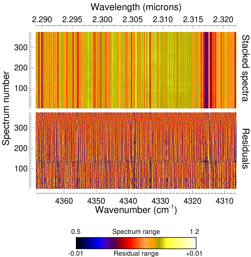
Figure 4: Top: Wavelength-calibrated and airmass corrected spectra for echelle order 33 on 26 August 2002. Bottom: Spectral residuals ($r_{\lambda t}$) after digital and Fourier filtering. The color bar shows the range of displayed intensities for the spectra and residuals.

There are two additional error sources in our spectra. First, there is the optical fringing with two distinct periods, noted by Brown et al. (2002). Both fringe systems are found in our data; however, they are less time-variable than experienced by Brown et al. (2002). Some of this optical fringing is removed by the digital filter which produces the $r_{\lambda t}$. However, Fourier analysis of the $r_{\lambda t}$ data reveals that both fringe systems remain detectable. When the residual fringes’ amplitudes exceed 0.25 in the log of the average power spectrum per echelle order per night, Fourier notch filters remove them. Second, extra noise is ubiquitous near the Nyquist frequency (0.5 cycles per pixel) in the power spectra of the $r_{\lambda t}$ with $\lambda$ varying. This probably derives from the array detector electronics. We remove it prior to the digital filter step by zeroing the Nyquist frequency in the Fourier spectrum. Figure 4 presents the stacked, wavelength-coincident spectra and the $r_{\lambda t}$ values for echelle order 33 on 26 August 2002, as false color images.

A complete understanding of the errors requires comparing the distribution of $r_{\lambda t}$ to a normal error curve, and also examining whether the noise power per unit bandwidth is constant (white noise). Although the error level varies with time and wavelength, the ratio of the individual residual values to their expected error, $\frac{r_{\lambda t}}{\sigma_{\lambda t}}$, should approach a Gaussian error distribution, with a standard deviation of unity. Figure 5 (upper panel) shows this distribution totaled over all 3 nights and all 3 echelle orders, on a log scale. Within $3\sigma$ this distribution is very close to the Gaussian error curve. However, the data exhibit an excess of points in the wings beyond $\pm 3\sigma$. Specifically, 0.5% of the $3.02\times 10^{6}$ points lie beyond $3\sigma$, and 0.05% are beyond $4\sigma$. A Gaussian distribution predicts 0.27% and 0.006% beyond $3\sigma$ and $4\sigma$ respectively. Using a Monte-Carlo simulation, we verified that the number of excess points in the wings of the data distribution are not sufficient to have a significant impact on our results, nor to affect our error analysis significantly, particularly since they are uncorrelated with transit phase. A more serious problem is the fact that the noise power per unit bandwidth is not constant, i.e. the 1/f character previously mentioned. We compute the power spectrum of each $r_{\lambda t}$ series, with $t$ varying, using a Lomb-Scargle algorithm (Press et al., 1994). The average of these power spectra for all $\lambda$ over all three nights is shown as the lower panel of Figure 5. The sharp increase in noise power below $\sim$ 2 cycles per night is quite evident; this increased noise at low frequencies would be about 2 times worse (0.3 in the log) without the digital filter technique described above.

4.4 Validation Using Fake Signals

In order to verify that our analysis is sensitive to the low levels of absorption expected in transit spectra, we have injected fake signals into the data and recovered them with our analysis procedures. The first fake signal is generated from the CO template spectrum of the fiducial model (Figure 1, solid line), Doppler shifted into the frame of the planet, and convolved to NIRSPEC spectral resolution. We adopted a heliocentric radial velocity for the system of $V_{r}=-14.76$ km sec^-1 (Nidever et al., 2002), and a planetary orbital velocity amplitude of 142 km sec^-1. The orbital period and transit times are very precisely known (Wittenmeyer et al., 2002; Schultz et al., 2003; Charbonneau et al., 2003), and we corrected for the Earth’s orbital motion, both in radial velocity and light travel time. A second fake signal is generated using the CO+water template spectrum (Figure 1, dotted line), and similarly transformed to the frame of the planet. We injected the fake signals into the data after the wavelength calibration, but before the digital filter and fringe removal. We therefore analyze three sets of data in parallel: the real data, and two copies of the real data with injected fake signals. Each of these data sets is analyzed against a grid of template spectra, where we offset the temperature in the model atmosphere, and vary the cloud height. In some cases we also set the CO mixing ratio to zero on the anti-stellar hemisphere of the planet, to simulate the worst-case effect of a large diurnal temperature difference.

4.5 The Stellar Spectrum

Our spectra contain significant information concerning the spectrum of the star, i.e. HD 209458a. Two aspects of the stellar spectrum are relevant to the transit analysis. First, we have searched for stellar CO absorption. In the solar spectrum, the first overtone CO features are relatively prominent, having line depths, when convolved to NIRSPEC resolution, of $\sim 6$%. Stellar lines are removed by the procedures that compute the $r_{\lambda t}$ residuals, so we have to identify them prior to removal of telluric lines. Also, stellar lines are not significantly modulated by the transit. Hence, they are somewhat difficult to detect. We therefore overlaid and averaged 26 lines of stellar CO lying in good telluric transmission windows. We see no evidence of a CO signature in the stacked spectra, with the confusion limit being determined by the telluric background at the $\sigma\sim 0.5$% level. CO lines of solar strength would be easily seen ($\sim 12\sigma$), but HD 209458a shows no detectable CO features. We considered whether the system might be lacking in carbon and/or oxygen, but the star has normal metallicity (Mazeh et al., 2000), and 2- to 3$\sigma$ evidence for both carbon and oxygen is seen in the planet’s UV transit spectrum (Vidal-Madjar et al., 2004). It is more likely that the non-appearance of stellar CO is related to the temperature of HD 209458a, which is slightly hotter than the sun (Mazeh et al., 2000; Ribas et al., 2003).

Although stellar CO is not detected in our spectra, we do detect the few stellar atomic lines that are expected. We used 5 atomic lines to derive the star’s radial velocity. We identified the lines using the Livingston and Wallace (1991) solar atlas, and fit parabolas to their line cores in both our Keck spectra and the solar atlas convolved to NIRSPEC resolution. On this basis we derive a heliocentric radial velocity for the system of $-15.4\pm 0.5$ km sec^-1, agreeing with the more precise Nidever et al. (2002) value, within our error. This serves as an independent check on our velocity transformation between the planet frame and the heliocentric frame.

4.6 Transit Spectrum Amplitudes and Transit Curve Fit

For each observed spectrum (at time $t$), we determine the degree to which the template transit spectrum ($d_{\lambda}$) is present in the $r_{\lambda t}$ values. We Doppler shift the template spectrum to the frame of the planet, convolve it to NIRSPEC resolution (see above), and filter it exactly as we filter the data. This transformed and filtered template spectrum ($d^{\star}_{\lambda}$) is used as the independent variable, with the $r_{\lambda t}$ values as the dependent variable, in a linear regression at each $t$:

$$r_{\lambda t}=z+a(t)d^{\star}_{\lambda},$$ (1)

where $z$ is a zero-point constant having no significance, and $a(t)$ is the statistical best-estimate of the amplitude of the template transit spectrum in the $r_{\lambda t}$ at that time (this treatment follows Richardson et al., 2003a). If the template spectrum is an exact description of the planet’s transit spectrum, then the $a(t)$ will lie on a transit curve which is zero out of transit and dips to -1 during transit (the negative sign denotes absorption, the $d_{\lambda}$ being proportional to the blocking area). As an added dimension to this calculation, we vary the assumed heliocentric radial velocity of the HD 209458 center of mass, by up to $\pm 235$ km sec^-1 ($\pm 50$ pixels), and we tabulate $a(t)$ for each $V_{r}$. Since line structure in the template corresponds to entirely different pixels in the data as $V_{r}$ is varied significantly, this added dimension serves to check the errors and significance of our results.

For the 26 August data, our first 80 spectra showed particularly troublesome uncontrolled grating motion. We found a systematic error in results based on these data, evident as a correlation between the spectrum shift and the $a(t)$. These 80 spectra were all taken prior to the start of transit. Since this portion of the transit curve is adequately sampled by other nights, we have deleted the first 80 spectra taken on 26 August from our analysis, as noted in Sec. 2.

We input the $\sigma_{\lambda t}$, $\sigma_{\lambda t}^{l}$, and $\sigma_{\lambda t}^{h}$ values to the least squares fits in order to estimate the errors in the $a(t)$ over the corresponding bandwidths, denoted ${\sigma}_{a}$, ${\sigma}_{a}^{l}$, and ${\sigma}_{a}^{h}$. The ${\sigma}_{a}$ are typically as large, or larger, than the amplitude itself (SNR$\lesssim$ 1). Nevertheless, the linearity of the analysis preserves the fidelity of the signal when the amplitudes from 1077 spectra are considered, and the expected SNR on the transit curve becomes sufficient to expect detection of CO absorption.

Fitting a theoretical transit curve to the $a(t)$ vs. time implicitly involves averaging them. This requires proper accounting for the errors as a function of frequency. For example, spectra taken in quick succession will produce an average $a(t)$ whose high frequency error of the mean decreases as the inverse square root of their number. But averaging spectra over brief intervals will not similarly reduce the low frequency errors, which can be correlated over short times. We are not aware of any rigorous methodology for treating non-white quasi-Gaussian errors in data analysis. We therefore implement the approach of approximating the full Fourier spectrum by two frequency bands, above and below 2 cycles per hour. We average the $a(t)$ for each night in 15-minute bins (0.003 in phase). Within a given bin on a given night, the high frequency errors apply, and the low frequency errors apply when comparing one bin to another. The binning involves a weighted average: within bin $i$ on night $j$ the $a(t)$ are weighted by the inverse square of their ${\sigma}_{a}^{h}$. The error associated with the average of bin $i$ on night $j$ is given as:

$$\sigma_{ij}=(\sum({\sigma}_{a}^{h})^{2}/N^{2}+({\sigma}_{a}^{l})^{2})^{\frac{1}{2}},$$ (2)

where the sum extends over the $N$ amplitudes in bin $ij$ and ${\sigma}_{a}^{l}$ is the typical low frequency error common to all points in the bin (the low frequency errors do not vary strongly within each $ij$ bin). Eq.(2) is easily derived from first principles, and we have verified it using numerical simulations. A grand average amplitude at phase $i$ results from combining bins at all $j$ (all nights), weighting the $ij$ bin averages by the inverse square of $\sigma_{ij}$. We similarly combine the $\sigma_{ij}$ to yield the error for the grand average amplitude at phase $i$.

We fit a theoretical transit curve to the grand average amplitudes and their errors. The shape of the theoretical transit curve is generated by numerically simulating the passage of the planet across a limb-darkened star, and the depth is normalized to unity, to be consistent with the amplitude retrievals (see above). The stellar and planet parameters were adopted from Brown et al. (2001), and the stellar limb-darkening at 2 $\mu$m was taken from the solar observations of Pierce et al. (1950).

5 Results

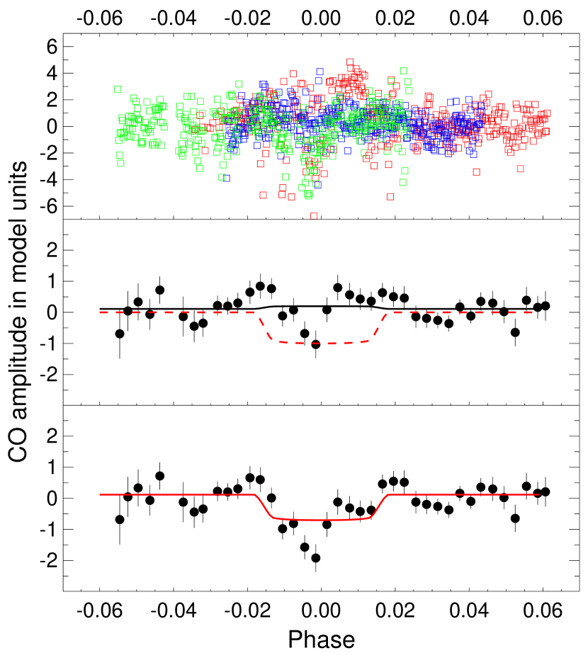
Figure 6: Results for the carbon monoxide transit depth for the fiducial model, having cloud tops at 37 mbar. Top: Retrieved CO amplitudes for all 1077 spectra over 3 observed transits (error bars supressed), red = 19 August, blue = 26 August, green = 2 September. Middle: Data binned by orbital phase (bin width 0.003), with error bars. The black solid line is the least squares fit of the transit curve, having depth $-0.09\pm 0.14$ in units of the fiducial model (i.e., no transit CO signal). The red dashed line is a forced fit of transit depth of unity, i.e. CO absorption during transit equal to the fiducial model. Bottom: The recovery of a fake signal input with CO transit depth of unity, and recovered at depth $0.82\pm 0.14$. Phase=0 is the center of transit.

Figure 6 plots the retrieved CO amplitudes, $a(t)$, for the fiducial model vs. phase. The 1077 individual $a(t)$ are shown in the top panel, with error bars supressed for clarity, but with different colors used for the three nights. The middle panel shows the grand average amplitudes binned over phase (bin width =0.003), with error bars added. To clarify our sign conventions, recall that points with negative amplitudes denote absorption. We fit a transit curve dipping to negative values during transit, so the fit of a negative curve to negative CO amplitudes should retrieve a positive depth (+1.0 if the fiducial model is correct). The transit curve is fit to the binned amplitudes in the middle panel, giving a depth of $-0.09\pm 0.14$ in model units, i.e. no evidence of CO absorption matching our template spectrum during transit. The solid line shows this best fit. The square root of the reduced chi-squared of the fit, $\sqrt{\chi^{2}/M}=1.19$, where $M$ is the number of degrees of freedom. Hence, the scatter in the binned amplitudes is somewhat greater than the error bars, which result from propagating the error in the $r_{\lambda t}$ values consistently through our linear analysis. The dashed red line in the middle panel shows a transit amplitude of unity, which is obviously incompatible with the data.

The lower panel of Figure 6 shows the binned fake data with transit curve fit. Our analysis recovers 82% of the input signal, with a least squares best fit transit depth of $0.82\pm 0.14$; this transit is shown as the solid red line. Note that only the relative depth of the transit curve is significant in these fits: the zero point displacement in amplitude units has no significance.

The 1/f noise in the $r_{\lambda t}$ produces a noticeable signature on Figure 6. Slow variations are evident in the top panel, giving the points in each color a quasi-patterned appearance. These variations ultimately derive from the variability of the terrestrial atmosphere. To investigate the error and significance of our result further, Figure 7 shows the depth of the best fit transit curve vs. the heliocentric $V_{r}$ of the HD 209458 center of mass (re-doing the analysis of the $r_{\lambda t}$ for each assumed $V_{r}$). The dispersion of the waveform shown on Figure 7 should be the same as the average error associated with the transit curve depth ($\sim 0.14$). The Figure 7 dispersion is 0.22; if we use this more conservative value as the error in transit curve depth, and considering the 82% efficiency of recovering the fake signal, the fiducial model is rejected at $\sim 4\sigma$ significance. The dashed line on Figure 7 shows the result from the fake CO signal, which is clearly detected at the correct $V_{r}$ of the system.

Our grid of template spectra provides several ways to explore physical reasons for the non-appearance of a CO transit. For example, we hypothesize a large temperature difference between the stellar-facing and anti-stellar hemispheres of the planet, with CO being absent on the anti-stellar side. As the template lines weaken, the error level increases, because the same data are being fit to smaller contrast in the template. When the error envelope, to some specified level of significance, expands to include a transit depth of 0.82 (the fake signal recovery level), that particular template spectrum can no longer be rejected. Setting the CO mixing ratio to zero on the anti-stellar side of the fiducial model produces a best fit transit depth of $-0.11\pm 0.16$, with the Figure 7 dispersion increasing to 0.25. This case is rejected at greater than $3\sigma$ significance, so removal of CO on the anti-stellar hemisphere has only a small effect on our results. The effect is small because the strong CO lines in the template are saturated.

Other physical effects that could account for our result are high clouds, or decreased temperature in the upper atmosphere of the planet. We have repeated our analysis over our entire grid of template spectra. None of the templates gives a significant detection of a CO transit. We compute the maximum cloud top pressure consistent with this null detection for each $\delta T$, by interpolating to find where the error envelope allows a transit depth of 0.82 (the fake signal transit depth). We take the size of the error envelope to be three times the formal error in transit depth (as in Figure 6 fits), or the maximum excursion in transit depth vs. $V_{r}$ (as in Figure 7), whichever is greater. The maximum cloud top pressure is plotted vs. the $\delta T$ added to the temperature profile in Figure 8. A separate relation is shown for the case when CO is absent on the anti-stellar hemisphere. Investigators who wish to make their own evaluation of models should use the criterion that the strong 2-0 R-branch lines between 4320 and 4330 cm^-1 have depths during transit less than 1.6 parts in $10^{4}$ in units of the stellar continuum (3$\sigma$ limit), at a spectral resolving power of 25,000. This observational criterion is weakly model-dependent because we derive it using a template spectrum (Figure 1) wherein the relative strengths of the CO lines vary slightly with temperature.

Water absorption has been included in one version of our model template (Figure 1, dotted line), and carried through our analysis as a second fake signal. To verify that water does not mask the presence of CO in our analysis, we first analyze the CO+water fake signal using the template containing only CO. This analysis yields a transit depth of $0.69\pm 0.14$. This is less than the $0.82$ depth recovered from the CO-only fake signal, albeit the same within the errors. Nevertheless, to guarantee maximum sensitivity to CO in the presence of water lines, we have analyzed the data with a full grid of CO+water templates. The CO+water template in the fiducial model recovers the fake CO+water signal with essentially the same efficiency (80%) that the CO-only template recovers the CO-only fake signal (82%). We have verified that our results (i.e., Figure 8) do not change significantly when the data are analyzed using the CO+water template grid.

6 Discussion

Our upper limit for CO is similar to the sodium detection (Charbonneau et al., 2002), in the sense that absorption from both Na and CO is significantly weaker than predicted by a fiducial model with cloud tops at 0.1/e bars (=37 mbar). Several published explanations for the weakness of sodium invoke some relatively specific mechanism that would not necessarily apply to CO (e.g., Barman et al., 2002). Our upper limit is interesting because fewer explanations can account for the weakness of both species. One of these viable explanations is the presence of high clouds. To be strictly consistent in comparing with the Charbonneau et al. (2002) interpretation of their sodium observations, we must refer to the highest temperature on Figure 8, $\delta T=+200$K. Charbonneau et al. (2002) followed Brown (2001) in using an early version of the Sudarsky et al. (2003) model that has $T=1150$K in the upper layers, 200 Kelvins hotter than is the model published by Sudarsky et al. (2003). At $\delta T=200$K, our results require a maximum cloud top pressure of 3.3 mbar (Figure 8). Using the Sudarsky et al. (2003) model without perturbation increases this to 5.7 mbar. Clouds occur at pressures as low as 1 mbar in some models. Not only do they reproduce the sodium result, they are helpful in accounting for the relatively large radius of the planet (Fortney et al., 2003; Burrows et al., 2003). However, the high forsterite cloud discussed by Fortney et al. (2003) is comprised of small particles ($\leq 0.5~{}\mu$m), whose visible opacity is dominated by scattering. At the much longer wavelength of the CO bands, scattering opacity by submicron particles will be greatly reduced (an issue discused by Brown, 2001), and such clouds may not suffice to explain our CO result. Indeed, Burrows et al. (2004) show a spectrum (their Figure 1) based on data from Fortney et al. (2003), that illustrates weakened sodium, but still shows prominent CO features. Cooler atmospheres would allow the IR-opaque cloud tops to occur at higher pressures (Figure 8), and might prove easier to reconcile with our results. Note that a cooler atmosphere for HD 209458b could also explain the non-detection of a 2 $\mu$m continuum peak by Richardson et al. (2003b).

It is interesting to note that even very cool temperatures for HD 209458b still require opaque clouds at pressures much less (i.e., greater geometric heights) than the point where a cloudless atmosphere becomes opaque in the tangent geometry. For example, Figure 8 requires cloud tops above 100 mbar even for a model 500K cooler than the Sudarsky et al. (2003) model. As we decrease the temperature in the Sudarsky et al. (2003) model, the mixing ratio of CO becomes negligible at the greatest heights, but a significant transit signature should persist from CO at higher pressures. Our null result therefore requires that clouds exist at an observable level in the atmosphere of HD 209458b, unless this planet is dramatically colder than current belief.

We have considered alternative interpretations of our result. Since the observed spectral resolution is high, a stringent requirement is that the line wavelengths be accurate. Fortunately, errors in line wavelengths are unlikely to be significant to our analysis. We inspected the much higher-resolution solar atlas (Livingston and Wallace, 1991), and were able to confirm wavelengths even for lines of insignificant importance to our template. For example, in the solar spectrum we find the 7-5 R(59) transition at 4083.797 cm^-1, vs. 4083.793 cm^-1 in our template (Goorvitch, 1994). We also consider the possibility that the absorbing levels of CO are depopulated high in the planetary atmosphere, i.e., not in local thermodynamic equilibrium (LTE). Note that departures from LTE are only significant as they affect the lower state of the absorbing transition; transit spectroscopy is insensitive to the upper state population. The strongest CO lines in our template are the P and R branches of the 2-0 and 3-1 bands, so it suffices for the $v=1$ level to be in LTE for our analysis to be valid. Ayres & Wiedemann (1989) discuss the radiative and CO-H₂ collisional rates for $v=1$ to $v=0$ relaxation. Using their Landau-Teller parameters for H₂ collisions, we calculate that the $v=1$ to $v=0$ collisional and radiative rates become comparable at 1 mbar. Therefore departures from LTE cannot solely explain our result, which requires weakening of CO at tens of mbar, where collisional rates dominate.

Figure 1: Theoretical transit depth for our fiducial model (cloud tops at 37 mbar) in the cases where we consider CO alone (solid line) and CO plus water (dotted line). The template spectra are plotted over the range covered by the 3 NIRSPEC echelle orders that contain CO, and they have been convolved to NIRSPEC resolution.

Figure 2: Average spectrum of HD 209458 in echelle order 33 on 26 August 2002. Most of the spectral structure is due to telluric lines of methane (solid tics) and water (dashed tics). Instrumental fringing is particularly noticeable in the 4320-4328 cm^-1 region.

Figure 3: Noise level $\sigma_{\lambda}$ achieved in echelle order 33 on 26 August 2002 vs. wavelength. We compute $\sigma_{\lambda}$ from the variation of residual spectral intensity, $r_{\lambda t}$, with $t$ (time) varying. Diamonds indicate wavelengths not utilized in subsequent analysis, due to the increased noise level near telluric lines (compare to Figure 2).

Figure 5: Top: distribution of residual values (solid line) compared to a Gaussian normal error distribution (dashed line). The bin size is 0.2 in ${r_{\lambda t}}/{\sigma_{\lambda t}}$. Note log scale used for the ordinate. Bottom: average power spectrum of the residuals, showing the increase in noise at low temporal frequencies. This average power spectrum has been normalized to a total power (area under the curve) = unity.

Figure 7: Transit depth from our analysis as a function of the heliocentric radial velocity ($V_{r}$) of the HD 209458 center of mass. The result from the fiducial model is plotted as a single point, with error bar from the fit. The dashed line shows recovery of the fake signal at the correct $V_{r}=-14.8$ km sec^-1.

Figure 8: Maximum cloud top pressure required to obtain consistency with our observations as a function of the temperature perturbation ($\delta T$) added to the Sudarsky et al. (2003) model. The dashed line gives the result of setting the CO mixing ratio to zero on the planet’s anti-stellar hemisphere.

References

- Alonso et al. (2004) Alonso, R., Brown, T. M., Torres, G., Latham, D. W., Sozzetti, A., Mandushev, G., Belmonte, J. A., Charbonneau, D., Deeg, H. J., Dunham, E. W., O’Donovan, F. T., & Stefanik, R. P. 2004, ApJ, 614, L153
- Ayres & Wiedemann (1989) Ayres, T. R., & Wiedemann, G. R. 1989, ApJ, 338, 1033
- Barman et al. (2002) Barman, T. S., Hauschildt, P. H., Schweitzer, A., Stancil, P. C., Baron, E., & Allard, F. 2002, ApJ, 569, L51
- Borysow (2002) Borysow, A. 2002, A&A, 390, 779
- Bouchy et al. (2004) Bouchy, F., Pont, F., Santos, N. C., Melo, C., Mayor, M., Queloz, D., & Udry, S. 2004, A&A, 421, L13
- Brown (2001) Brown, T. M. 2001, ApJ, 553, 1006
- Brown et al. (2001) Brown, T. M., Charbonneau, D., Gilliland, R. L., Noyes, R. W., & Burrows, A. 2001, ApJ, 552, 699
- Brown et al. (2002) Brown, T. M., Libbrecht, K. G., & Charbonneau, D. 2002, PASP, 114, 826
- Burrows et al. (2003) Burrows, A., Sudarsky, D. & Hubbard, W. B. 2003, ApJ, 594, 545
- Burrows et al. (2004) Burrows, A., Sudarsky, D., & Hubeny, I. 2004, in The Search for Other Worlds, eds. S. Holt & D. Deming, AIP Conference Series, (Melville, New York: American Institute of Physics), p. 143.
- Burrows and Sharp (1999) Burrows, A., & Sharp, C. M. 1999, ApJ, 512, 843
- Charbonneau et al. (2000) Charbonneau, D., Brown, T. M., Latham, D. W., & Mayor, M. 2000, ApJ, 529, L45
- Charbonneau et al. (2002) Charbonneau, D., Brown, T. M., Noyes, R. W., & Gilliland, R. L. 2002, ApJ, 568, 377
- Charbonneau et al. (2003) Charbonneau, D., Brown, T. M., Gilliland, R. L., & Noyes, R. W. 2003, paper presented at The Search for Other Worlds, eds. S. Holt & D. Deming, AIP Conference Series, (Melville, New York: Ameican Institute of Physics).
- Fortney et al. (2003) Fortney, J. J., Sudarsky, D., Hubeny, I., Cooper, C. S., Hubbard, W. B., Burrows, A., & Lunine, J. 2003, ApJ, 589, 615
- Goorvitch (1994) Goorvitch, D. 1994, ApJS, 95, 535
- Harrington et al. (2003) Harrington, J., Deming, D., Goukenleuque, C., Matthews, K., Richardson, L. J., Steyert, D., Wiedemann, G., & Zeehandelaar, D. 2003, in Scientific Frontiers in Research on Extrasolar Planets, eds. D. Deming & S. Seager, ASP Conference Series Vol. 294, (San Francisco: Astronomical Society of the Pacific), 471
- Henry et al. (2000) Henry, G. W., Marcy, G. W., Butler, R. P., & Vogt, S. S. 2000, ApJ, 529, L41
- Horne (1986) Horne, K. 1986, PASP, 98, 609
- Hubbard et al. (2001) Hubbard, W. B., Fortney, J. J., Lunine, J. I., Burrows, A., Sudarsky, D., & Pinto, P. 2001, ApJ, 560, 413
- Hui & Seager (2002) Hui, L. & Seager, S. 2002, ApJ, 572, 540
- Jorgensen et al. (2000) Jorgensen, U. G., Hammer, D., Borysow, A., & Falkgesgaard, J. 2000, A&A, 361, 283
- Konacki et al. (2003) Konacki, M., Torres, G., Jha, S., & Sasselov, D. D. 2003, Nature, 421, 507
- Konacki et al. (2004) Konacki, M., Torres, G., Sasselov, D. D., Pietrzynski, G., Udalski, A., Jha, S., Ruiz, M. T., Gieren, W., & Minniti, D. 2004, ApJ, 609, L37
- Lammer et al. (2003) Lammer, H., Selsis, F., Ribas, I., Guinan, E. F., Bauer, S. J., & Weiss, W. W. 2003, ApJ, 598, L121
- Liang et al. (2003) Liang, M.-C., Parkinson, C. D., Lee, A. Y.-T., Yung, Y. L., & Seager, S. 2003, ApJ, 596, L247
- Livingston and Wallace (1991) Livingston, L. W., & Wallace, L. 1991, An Atlas of the Solar Spectrum in the Infrared from 1850 to 9000 cm-1 (1.1 to 5.4 Microns), NSO Technical Report #91-001 (Tucson: National Solar Observatory)
- Marcy et al. (2003) Marcy, G. W., Butler, R. P., Fischer, D. A., & Vogt, S. S. 2003, in Scientific Frontiers in Research on Extrasolar Planets, eds. D. Deming & S. Seager, ASP Conference Series Vol. 294, (San Francisco: Astronomical Society of the Pacific), 1
- Mazeh et al. (2000) Mazeh, T., and 19 co-authors, 2000, ApJ, 532, L55
- McLean et al. (1998) McLean, I. S., et al. Proc. SPIE, 3354, 566
- Nidever et al. (2002) Nidever, D. L., Marcy, G. W., Butler, R. P., & Vogt, S. S. 2002, ApJS, 141, 503
- Noll et al. (1997) Noll, K. S., Geballe, T. R., & Marley, M. S. 1997, ApJ, 489, L87
- Partridge and Schwenke (1997) Partridge, H. & Schwenke, D. W. 1997, J. Chem. Phys. 106, 4618
- Pierce et al. (1950) Pierce, A. K., McMath, R. R., Goldberg, L., & Mohler, O. C. 1950, ApJ, 112, 289
- Pont et al. (2004) Pont, F., Bouchy, F., Queloz, D., Santos, N., Melo, C., Mayor, M., & Udry, S. 2004, A&A, in press, astro-ph/0408499
- Press et al. (1994) Press, W. H., Teukolsky, S. A., Vetterling, W. T., & Flannery, B. P. 1994, Numerical Recipes in C, (Cambridge: Cambridge University Press)
- Ribas et al. (2003) Ribas, I., Solano, E., Masana, E., & Gimenez, A. 2003, A&A, 411, L501
- Richardson et al. (2003a) Richardson, L. J., Deming, D., Wiedemann, G., Goukenleuque, C., Steyert, D., Harrington, J., & Esposito, L. W. 2003a, ApJ, 584, 1053
- Richardson et al. (2003b) Richardson, L. J., Deming, D., & Seager, S. 2003b, ApJ, 597, 581
- Sudarsky et al. (2003) Sudarsky, D., Burrows, A., & Hubeny, I. 2003, ApJ, 588, 1121
- Seager and Sasselov (2000) Seager, S. & Sasselov, D. D. 2000, ApJ, 537, 916
- Seager (2003) Seager, S. 2003, in Scientific Frontiers in Research on Extrasolar Planets, eds. D. Deming & S. Seager, ASP Conference Series Vol. 294, (San Francisco: Astronomical Society of the Pacific), 457
- Schultz et al. (2003) Schultz, A. B., Kochte, M., Kinzel, W., Hamilton, F., Jordan, I., Henry, G., Vogt, S., Bruhweiler, F., Storrs, A., Hart, H. M., Bennum, D., Rassuchine, J., Rodrigue, M., Hamilton, D. P., Welsh, W. F., Wittenmeyer, R., & Taylor, D. C. 2003, in Scientific Frontiers in Research on Extrasolar Planets, eds. D. Deming & S. Seager, ASP Conference Series Vol. 294, (San Francisco: Astronomical Society of the Pacific), 479
- Showman and Guillot (2002) Showman, A. P., & Guillot, T. 2002, A&A, 385, 166
- Vidal-Madjar et al. (2003) Vidal-Madjar, A., Lecavelier des Etangs, A., Desert, J.-M., Ballester, G. E., Ferlet, R., Hebrard, G., & Mayor, M. 2003, Nature, 422, 143
- Vidal-Madjar et al. (2004) Vidal-Madjar, A., Desert, J.-M., Lecavelier des Etangs, A., Hebrard, G., Ballester, G. E., Ehrenreich, D., Ferlet, R., McConnell, J. C., Mayor, M., & Parkinson, C. D. 2004, ApJ, 604, L69
- Wiedemann et al. (2001) Wiedemann, G. R., Deming, D., & Bjoraker, G. 2001, ApJ, 546, 1068
- Wittenmeyer et al. (2002) Wittenmeyer, R. A., Welsh, W. F., & Orosz, J. A. 2002, BAAS, 201, 46.11