AWM 4 - an isothermal cluster observed with XMM-Newton

Abstract

We present analysis of an XMM-Newton observation of the poor cluster AWM 4. The cluster is relaxed and its X-ray halo is regular with no apparent substructure. Azimuthally averaged radial spectral profiles suggest that the cluster is isothermal to a radius of at least 160 kpc, with no evidence of a central cooling region. Spectral mapping shows some significant temperature and abundance substructure, but no evidence of strong cooling in the cluster core. Abundance increases in the core, but not to the extent expected, and we find some indication of gas mixing. Modeling the three dimensional properties of the system, we show that ongoing heating by an AGN in the dominant elliptical, NGC 6051, is likely to be responsible for the lack of cooling. We also compare AWM 4 to MKW 4, a cluster of similar mass observed recently with XMM-Newton. While the two systems have similar gravitational mass profiles, MKW 4 has a cool core and somewhat steeper gas density profile, which leads to a lower core entropy. AWM 4 has a considerably larger gas fraction at 0.1$\times$$R_{\mathrm{200}}$, and we show that these differences result from the difference in mass between the two dominant galaxies and the activity cycles of their AGN. We estimate the energy required to raise the temperature profile of MKW 4 to match that of AWM 4 to be 9$\times$10⁵⁸ erg, or 3$\times$10⁴³ $\mbox{~{}erg}\mbox{~{}s}^{-1}$ for 100 Myr, comparable to the likely power output of the AGN in AWM 4.

1 Introduction

AWM 4 is a poor cluster consisting of $\sim$30 galaxies centred on the giant elliptical NGC 6051 (Koranyi & Geller, 2002). The association of galaxies was first identified in the survey of Albert et al. (1977), and the presence of a deep potential well was later confirmed by X–ray observations (Kriss et al., 1983). Of the identified galaxies in the group, most are absorption line systems, with a strong concentration of early-type galaxies toward the core (Koranyi & Geller, 2002). The group is apparently relaxed, with a smooth velocity distribution about a mean redshift of $cz$=9520 $\mbox{~{}km}\mbox{~{}s}^{-1}$. In conjunction with the morphology segregation, this suggests that it has been undisturbed by major interactions for some time.

The dominant elliptical in the cluster is considerably more luminous than the galaxies around it, with a difference in magnitude above the second-ranked galaxy of $M_{12}$=1.426. NGC 6051 is well described by an r${}^{\frac{1}{4}}$ law surface brightness profile, and does not show signs of an extended stellar envelope (Schombert, 1987). NGC 6051 has a powerful active nucleus (4C +24.36), with radio lobes extending out roughly along the minor axis of the galaxy. There is no sign of a central point source at other wavelengths, suggesting that the axis of the AGN jets is in the plane of the sky, and that the central engine is highly absorbed. The galaxy major axis is roughly aligned with that of the galaxy distribution, and that of the X–ray halo. Table 1 gives details of the position and scale of the cluster and its dominant galaxy.

The cluster has been observed in the X-ray band previously, by the Einstein, ASCA and ROSAT observatories. These observations have shown it to be extended, regular, and relatively luminous. The temperature of the halo gas has been shown to be $\sim$2.5 keV (Kriss et al., 1983; Finoguenov et al., 2001), and several estimates of the mass of the system have been made. These agree reasonably well with the mass estimated from the galaxy distribution, $\sim$9$\times$10¹³ $M_{\odot}$ within 600 kpc (Koranyi & Geller, 2002). Analysis of the ASCA data for the cluster shows it to have a relatively flat temperature profile, though the poor spatial resolution of the instrument prevents the identification of any small scale cooling in the core of the cluster.

AWM 4 lies at the low end of the mass and temperature range usually associated with clusters. While more massive clusters have been relatively thoroughly studied and are currently receiving much attention, the lower luminosities of galaxy groups have made the exploration of their properties more difficult. Systems at the border between these two classes are particularly interesting, in that they may shed light on the mechanisms behind the differences between clusters and groups. AWM 4 is also of interest because of the large radio source associated with NGC 6051. Several Chandra studies in larger systems have found evidence that AGN jets can evacuate cavities in the hot intra-cluster medium (ICM), and may have a part in regulating cooling (e.g., Fabian et al., 2000; McNamara et al., 2000). The ICM in AWM 4 is cooler than in these more massive systems, and this gives us an opportunity to observe the effects of a powerful AGN on a relatively small cluster.

In this paper, we use a recent XMM-Newton observation of AWM 4 to study the structure of the cluster halo. Section 2 describes the observation and the reduction of the data, and Section 3 describes our data analysis and our main results. We discuss these in Section 4, and compare them with results for other systems. Our conclusions are given in Section 5. Throughout the paper we assume $H_{\mathrm{0}}$=75 $\mbox{~{}km}\mbox{~{}s}^{-1}\mbox{~{}Mpc}^{-1}\,$ and normalise optical luminosities to the B-band luminosity of the sun, $L_{B\odot}$=5.2$\times$10³² $\mbox{~{}erg}\mbox{~{}s}^{-1}$. Abundances are measured relative to the abundance ratios of Anders & Grevesse (1989). These differ from the more recent ratios given by Grevesse & Sauval (1998) in that the abundance of Fe is a factor of $\sim$1.4 lower. This means that our measured abundances are underestimated by a factor of $\sim$1.4 when compared with those estimated using the more recent ratios. This should be noted when making comparisons with other results.

R.A. (J2000)	16 04 57.0
Dec. (J2000)	+23 55 14
Redshift	9520 $\mbox{~{}km}\mbox{~{}s}^{-1}$
Distance ($H_{\mathrm{0}}$=75)	126.9 Mpc
1 arcmin =	36.9 kpc
NGC 6051 $D_{\mathrm{25}}$ radius	28.6 kpc

Table 1: Location and scale for AWM 4.

2 Observation and Data Reduction

AWM 4 was observed with XMM-Newton during orbit 573 (2003 January 25-26) for just over 20,000 seconds. The EPIC MOS and PN instruments were operated in full frame and extended full frame modes respectively, with the medium filter. A detailed summary of the XMM-Newton mission and instrumentation can be found in Jansen et al. (2001, and references therein). The raw data from the EPIC instruments were processed with the most recent version of the XMM-Newton Science Analysis System (sas v.5.4.1), using the epchain and emchain tasks. After filtering for bad pixels and columns, X–ray events corresponding to patterns 0-12 for the two MOS cameras and patterns 0-4 for the PN camera were accepted. Investigation of the total count rate for the field revealed a short background flare in the second half of the observation. Times when the total count rate deviated from the mean by more than 3$\sigma$ were therefore excluded. The effective exposure times for the MOS 1, MOS 2 and PN cameras were 17.3, 17.4 and 12.7 ksec respectively.

Images and spectra were extracted from the cleaned events lists with the sas task evselect. For simple imaging analysis, the filtering described above was considered sufficient. Event sets for use in spectral analysis were further cleaned using evselect with the expression ‘(FLAG == 0)’ to remove all events potentially contaminated by bad pixels and columns. All data within 17^′′ of point sources were also removed, excluding the false source detection for the core of NGC 6051. We allowed the use of both single and double events in the PN spectra, and single, double, triple and quadruple events in the MOS spectra. Response files were generated using the sas tasks rmfgen and arfgen.

[!h] Dataset	MOS 1	MOS 2	PN
Blank field	0.0312	0.0282	0.121
Telescope closed	0.142	0.172	0.609

Table 2: Scaling factors used in creation of background spectra and images. The factors show the scaling between the source dataset and the blank field or telescope closed data for each instrument.

Background images and spectra were generated using the “double subtraction” method (Arnaud et al., 2002; Pratt et al., 2001). The “blank field” background data sets of Read & Ponman (2003) and the “telescope closed”, particles only data sets of Marty et al. (2002) form the basis of this process. Background images are generated by scaling the “closed” data to match the measured events outside the telescope field of view. The “blank” data are then scaled to match the observation exposure time, and a “soft excess” spectrum calculated by comparison of this scaled background to the low energy observed spectrum in the outer part of the detector field of view. The source does not extend to the outer part of the field of view, so the soft excess spectrum should measure only the difference in background soft emission between the “blank” data and that for the target. The various background components can then be combined to form the background images. A similar process is used to create background spectra, again scaling the “blank” data to match the observation, and correcting for differences in the soft background component using a large radius spectrum. Scaling factors used to correct the “blank” and “closed’ data are shown in table 2. The “soft excess” spectrum for the PN resembles a 0.6 keV Bremsstrahlung model, but while the MOS spectra are consistent with this they are of poorer quality and contain elements which appear to be associated with spectral lines in the background, most notably the 1.55 keV Al-K fluorescent line. Neither PN nor MOS “soft excess” spectra can be accurately represented by a simple model, as is to be expected given the method by which they are constructed. However, the apparent low temperature of the spectrum confirms that we are not including cluster emission in the background, as ROSAT spectra suggest that at the radius used, the cluster temperature is $\sim$1.6 keV (Helsdon & Ponman, 2000). The normalisation of the Bremsstrahlung model is $\sim$7.6$\times 10^{-8}$ arcmin^-2 for the PN and $\sim$1.1 $\times 10^{-8}$ arcmin^-2 for the MOS.

In some cases, where the signal-to-noise of our spectra was relatively low, we tested the quality of these “double” background spectra to determine whether we might be introducing error through the scaling process. We selected an annular region in the observation data set, at large radius where the source contribution should be negligible, and used it as an alternate background. We then compared the resulting spectral fits. In all cases the fits were similar, with no qualitative difference introduced by the use of the “double” background spectra. We therefore consider these to be an accurate measure of the background in all cases.

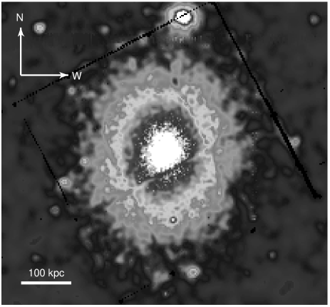
Figure 1: Adaptively smoothed X–ray image of AWM 4, combining data from the PN and MOS cameras.

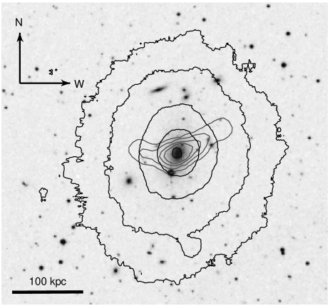
Figure 2: Digitized Sky Survey image of the core of AWM 4 with X–ray and radio contours superimposed. X–ray contours (black) are taken from our MOS images, while the radio contours (shown in grey) are from the VLA First 20cm survey. Higher resolution radio contours can be seen in Figure 8.

3 Results

Figure 1 shows an exposure and vignetting corrected mosaiced image of AWM 4, combining data from the PN and two MOS cameras. The image was smoothed using the sas task asmooth with smoothing scales chosen to achieve a signal-to-noise ratio of 10. The X-ray halo is highly extended and elliptical, with the major axis running approximately north-south. Ignoring the distortion introduced by the PN chip gaps, the cluster appears quite regular, with no major substructure. Several point-like sources are visible in the field, as well as the bright background Seyfert 1 galaxy J160452.8+240235 (Véron-Cetty & Véron, 2001), visible to the north of the cluster near a chip gap. The extent of the radio source associated with NGC 6051 can be seen in Figure 2. The two lobes extend well beyond the central galaxy, to at least 70 kpc eastward and 85 kpc to the northwest.

3.1 Two-dimensional surface brightness modeling

We created images in the 0.5-3.0 keV band for each detector, with associated background images, and exposure maps. We used the sas task calview to produce on-axis PSF images for each camera in this energy band. All images were binned to 4.4^′′ pixels. We then simultaneously fit these images using sherpa (running in ciao v2.3). As the data contain numerous pixels which have small numbers of (or zero) counts, we used the Cash statistic (Cash, 1979). This requires us to model the background, and we use flat models, with the normalisation free to vary independently for each camera. This will introduce some inaccuracies, as the background is not flat. However, the variation relative to the source is small, and using a background model allows us effectively to ignore small variations in the background data sets. The Cash statistic does not provide an absolute measure of the goodness of the fit, so we used the residual images and azimuthally averaged radial profiles to check the fit quality.

We initially fit a single beta model, which was reasonably successful, and allowed us to determine the position angle and ellipticity of the group halo. The background models were allowed to vary freely during fitting. However, it was clear from the radial profile that the fit did not successfully model the inner part of the halo, and we therefore introduced a second beta model, which we constrained to be circular. This produced a satisfactory model of the halo, with no major residuals. Parameters of these fits are given in Table 3. Radial surface brightness profiles for the two fits are shown in Figure 3.

Fit	rcore	$\beta_{fit}$	axis ratio	position angle	amplitude	rcore,2	$\beta_{fit,2}$	amplitude
	(kpc)			(degrees)		(kpc)
1 component	67.32${}^{+0.29}_{-2.42}$	0.672${}^{+0.011}_{-0.002}$	1.20$\pm$0.01	174.56${}^{+0.93}_{-0.94}$	7.702	-	-	-
2 component	96.74${}^{+19.13}_{-1.66}$	0.708${}^{+0.054}_{-0.005}$	1.22${}^{+0.04}_{-0.02}$	174.48${}^{+2.39}_{-2.01}$	4.155	33.58${}^{+20.58}_{-9.03}$	0.998${}^{+0.749}_{-0.347}$	7.657

Table 3: Parameters with 1$\sigma$ errors for the best fitting surface brightness models. Note that the 1-component fit, while adequate at high radii, is a poor fit in the core. Errors for each model were estimated with all parameters shown in the table free for perturbation. Position angle is measured anti-clockwise from north.

Figure 3: Radial surface brightness profiles for the 2-component (left) and 1-component (right) models. In both cases the data, which for the purpose of the profile is taken from the MOS 1 image, is marked by black points with (1$\sigma$) error bars. In the 1-component plot the fitted beta model and flat background model are marked by solid lines. In the 2-component plot the combined model is marked by a solid line, while the model components and the background are marked by dashed lines. Note that each model component has the background added to it in this plot, hence the inner beta model curves to meet the background at large radii.

Our models show a somewhat steeper profile than has previously been obtained assuming azimuthal symmetry. Fits to Einstein IPC data using a single beta model gave $\beta_{fit}$$\sim$0.6 and a core radius of $\sim$130 kpc (Jones & Forman, 1999), for a region of interest $\sim$960^′′ (590 kpc) in radius. Using ROSAT PSPC data, Finoguenov et al. (2001) found a similar slope, $\beta_{fit}$=0.62$\pm$0.02, and a rather smaller core radius, r_c=68.7$\pm$2.8 kpc. However, a small region in the center of the group was excluded in the ROSAT analysis, in order to avoid biases associated with a central cooling region. It seems possible that the differences between our fits and those from Einstein and ROSAT might arise from the poorer spatial resolution of the instruments used, the removal of the core of the group, and the differences in size of field used in the fits.

3.2 Spectral modeling

Given the estimate of the ellipticity and angle of the group halo, we were able to choose a region from which to extract an overall spectrum. We chose a region with minor axis 260^′′ (158 kpc) and ellipse parameters as in the 1-component surface brightness fit. We then extracted spectra for this region from all three cameras, and generated appropriate background files. The resulting spectra were simultaneously fitted using xspec (v11.2.0ab). We ignored energies less than 0.4 keV and greater than 8.0 keV, where the calibration of the EPIC instruments is known to be questionable. An example of the spectra and fitted model can be seen in Figure 4.

The three spectra were adequately modeled by both the MEKAL (Liedahl et al., 1995; Kaastra & Mewe, 1993) and APEC (Smith et al., 2001) hot plasma codes, leading us to believe that the X-ray emission of the group is dominated by the contribution of the gaseous halo. Multi-temperature models were not required, suggesting that the halo is roughly isothermal. $N_{\mathrm{H}}$ was held at the Galactic value (5$\times$10²⁰ cm²) in these fits. Details of the best fitting models are given in Table 4. The agreement between the APEC and MEKAL models is good, and the abundances of most elements are quite comparable. One noteworthy point is the difference in abundance between Si and Fe, with Si being more abundant than Fe at $>$90% significance. We note however that this would be affected were we measure abundance relative to the ratios of (Grevesse & Sauval, 1998), as discussed in Section 1.

Parameter	MEKAL	APEC
kT	2.56$\pm$0.06	2.55${}^{+0.05}_{-0.06}$
Zavg	0.33${}^{+0.14}_{-0.11}$	0.47${}^{+0.16}_{-0.14}$
O	0.16${}^{+0.12}_{-0.11}$	0.18${}^{+0.15}_{-0.13}$
Si	0.54${}^{+0.11}_{-0.10}$	0.57$\pm$0.11
S	0.26${}^{+0.13}_{-0.12}$	0.27$\pm$0.13
Fe	0.35${}^{+0.03}_{-0.04}$	0.36$\pm$0.04

Table 4: Best fit parameters for spectral fits to the integrated spectrum of AWM 4, extracted from a region of minor axis 260^′′ (158 kpc), major axis 312^′′ (190 kpc) and ellipse parameters taken from the 1-component surface brightness model. The ranges shown are the 90% error bounds for each parameter. Temperature (kT) is in keV, and all metal abundances are relative to solar. Z_avg is the average abundance of all metals not listed individually.

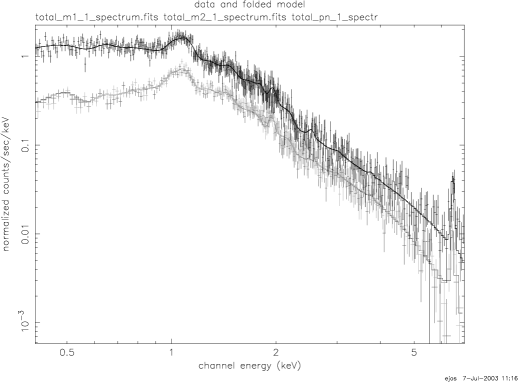
Figure 4: EPIC PN (upper, black), MOS1 and MOS 2 (lower, grey) spectra of AWM 4, as used in our overall spectral fit to the cluster.

We estimate the total luminosity within the region of interest in three energy bands from the best fit MEKAL model. The luminosities are Log $L_{\mathrm{X}}$=42.96 $\mbox{~{}erg}\mbox{~{}s}^{-1}$ (0.5-2 keV), Log $L_{\mathrm{X}}$=43.22 $\mbox{~{}erg}\mbox{~{}s}^{-1}$ (0.4-8 keV, the energy band used in fitting) and Log $L_{\mathrm{X}}$=43.31 $\mbox{~{}erg}\mbox{~{}s}^{-1}$ (0.1-12 keV). The relatively small change between the last two values suggest that the 0.1-12 keV luminosity is a good approximation of the bolometric X-ray luminosity.

3.2.1 Radial profiles

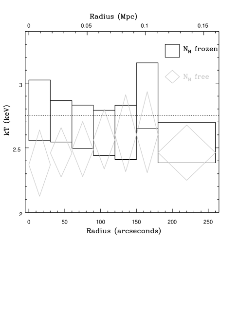
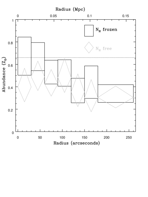
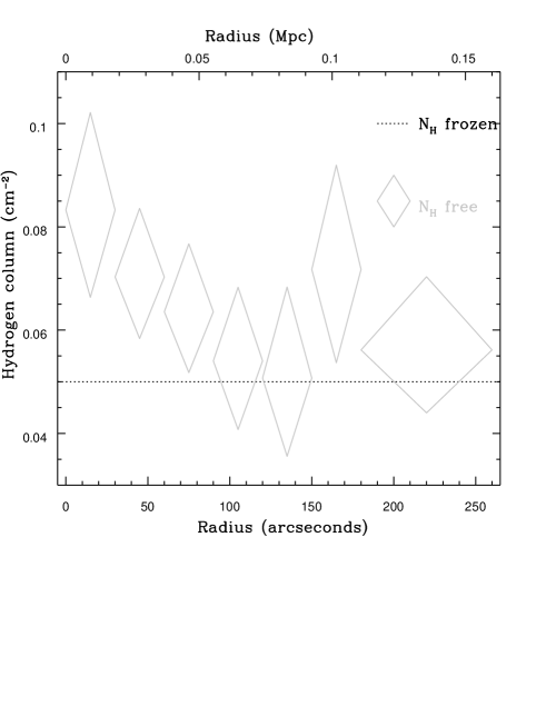
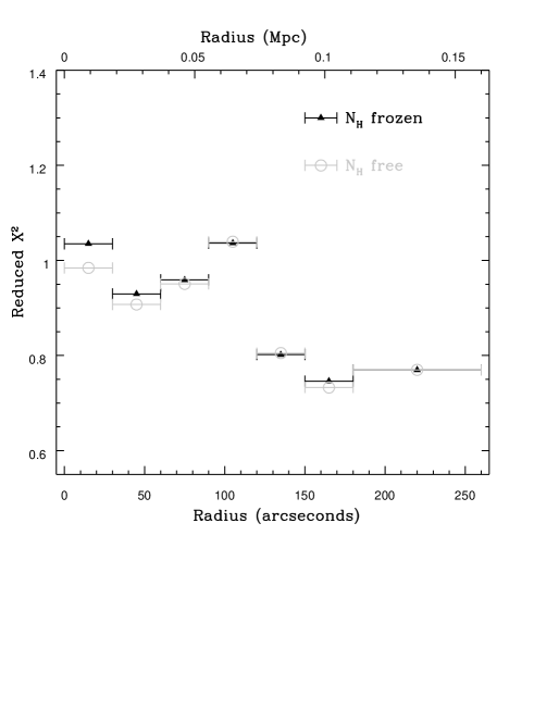
Figure 5: Radial profiles of projected temperature, abundance, hydrogen column and fit statistic (reduced $\chi_{\nu}^{2}$) for AWM 4. In each plot, numbers along the upper axis show radius in Mpc, while those on the lower axis show radius in arcseconds. All radii are for the minor axis of the elliptical region. Grey symbols refer to fits carried out with hydrogen column free to vary, black symbols to those where column is held at the Galactic value. All regions denote 90% errors. The dotted line in the $N_{\mathrm{H}}$ plot shows the Galactic column value. The dotted lines in the kT and abundance plots show the approximate values of these parameters measured by ASCA (Finoguenov et al., 2001).

Using elliptical annuli, we generated spectra in radial bins. Again, spectra for all three EPIC instruments were simultaneously fitted, using an absorbed MEKAL model. Fits with hydrogen column fixed at the Galactic value (5.00$\times$10²⁰ cm²), and with column free to vary were performed. The resulting profiles are shown in Figure 5.

The first and most important feature of these profiles is that the group appears to be isothermal. The temperature is consistent with that derived from ASCA (Finoguenov et al., 2001). The abundance shows some evidence of decline with increasing radius, but is consistent with the ASCA Fe abundance in all but the outermost bin. This is not unexpected, as the ASCAprofile has only 2 bins in the range we are interested in, values from which should be weighted averages of those we observe. The fits are statistically acceptable in all bins. The low fit parameters in the three outer bins reflect the reduced numbers of counts at larger radii. When the Hydrogen column is free to fit it varies by a factor of $\sim$1.7, but does not significantly improve the fits, except perhaps in the innermost bins. The two innermost bins are also where $N_{\mathrm{H}}$ has the largest effect on the fitted values of temperature and abundance, though the error regions are consistent.

If the fitted $N_{\mathrm{H}}$ in the three innermost bins is taken at face value, the excess hydrogen column above the measured Galactic value indicates a total hydrogen mass of 1.64$\times$10¹⁰$M_{\odot}$ within the cluster core. Unfortunately this cannot be ruled out by radio measurements. Only an upper limit on the neutral hydrogen mass is available from Hi measurements, $\leq$6.8$\times$10⁹$M_{\odot}$, and strong radio emission from NGC 6051 means that the error on this limit could be significant (Valentijn & Giovanelli, 1982). However, if there is intrinsic absorption then it must extend to a radius $>$55 kpc, approximately twice the $D_{\mathrm{25}}$ radius of the dominant galaxy. We cannot rule out an Hi cloud of this size, but as it seems unlikely, and its inclusion does not greatly improve our fits, we choose to assume that only Galactic absorption affects the data.

Our central bin is relatively large, with a radius of 30^′′ ($\sim$18.5 kpc), and it is possible that we would not resolve a small cooling region in the core of the dominant galaxy. NGC 6051 also hosts an AGN which, while not apparent in the surface brightness profile, might be contribute to the X-ray emission from the central bin. We therefore fitted additional models to the spectra from this bin, including 2-temperature plasma models, plasma + power law models, and cooling models such as VMCFLOW and CEVMKL. These were not successful. For the best fit two component models the power law or high temperature plasma component was always poorly constrained and made almost no contribution to the spectrum. The cooling models suggest that the gas has a very narrow range of temperatures and is certainly not cooling significantly. We therefore conclude that there is no significant cooling or temperature structure in the cluster core, and that the AGN in NGC 6051 must be heavily absorbed.

Using the same annuli we also fitted a deprojected spectral profile. The deprojection was carried out using the XSPEC projct model in combination with an absorbed MEKAL model. The hydrogen column was again held fixed at the Galactic value, and all metal abundances were tied. The resulting deprojected temperature and abundance profiles can be seen in Figure 6. As was to be expected, the errors are quite large, and the same general trends are seen in the projected and deprojected profiles. The temperature profile is consistent with isothermality, while the abundance profile declines with radius. The fits in the two outermost bins are somewhat better constrained than the inner four, so we performed further fits with the six bins grouped into two sets. The results of these fits are also shown in Figure 6 and the improvement in accuracy is clear. It is again clear that while temperature is consistent with isothermality, showing only a slight trend with radius, there is a decline in abundance at large radii.

We also fit projected radial spectra with the abundance of Fe and Si free to vary. All other metals were tied, but free to vary as a group. Hydrogen column was held fixed at the Galactic value. Given the lower numbers of counts at large radii, it was necessary to merge the two outermost bins to achieve a reliable fit. The results are shown in Figure 7. There is a marginal trend for a higher Si abundance in five of the six bins, but the difference is only significant (at the 90% level) in bin 4. Overall we cannot claim any significant difference in abundance between Fe, Si and other elements, and there is no trend with radius beyond the decline already noted. The Fe and Si abundances are consistent with the ASCA measurements of Finoguenov et al. (2001) in the core, but are a poorer match at larger radii. The outer bins are quite comparable to the abundances derived by Fukazawa et al. (1998), also from ASCA though these were measured at slightly larger radii than our data permit. Given the difficulties associated with ASCA analysis, particularly in a field containing a bright AGN, we consider the agreement acceptable.

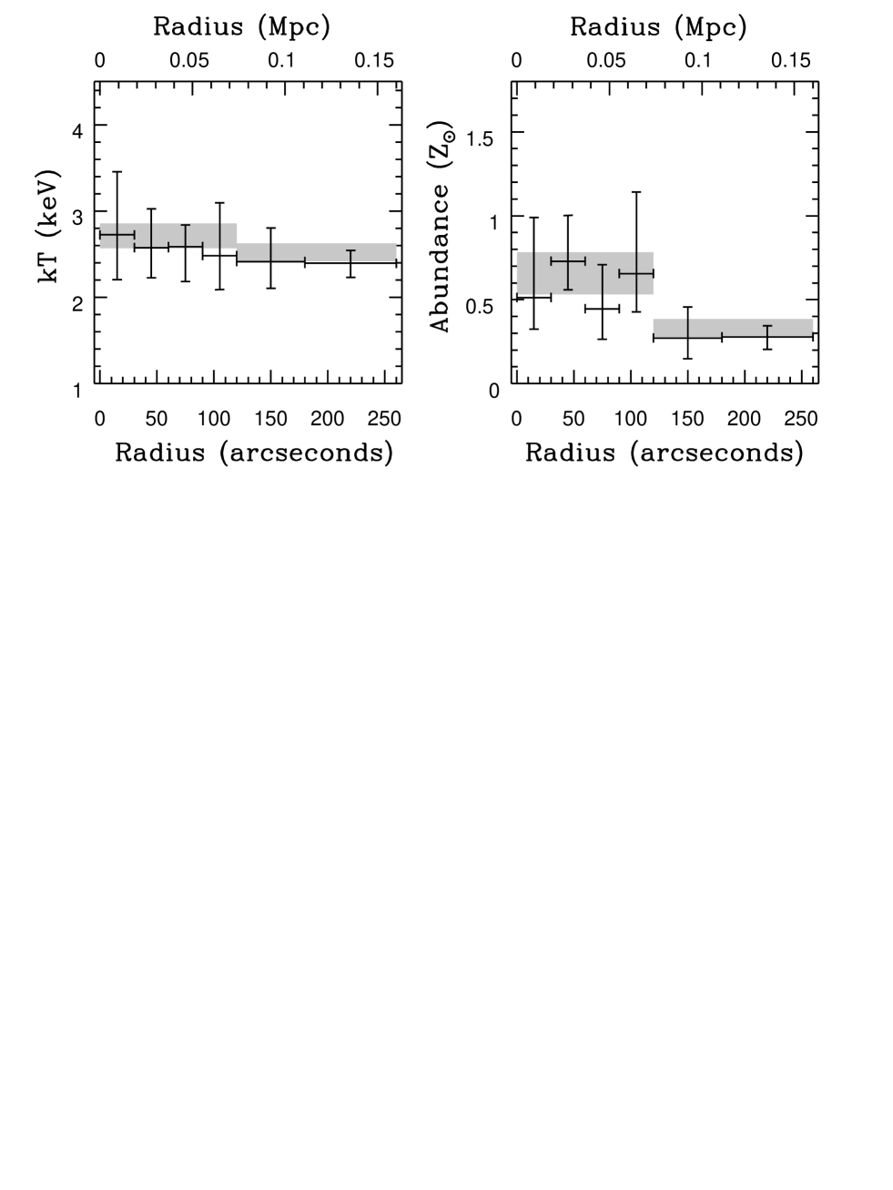
Figure 6: Radial profiles of deprojected temperature and abundance. Crosses mark free fits to the six bins, and shaded grey regions mark fit with the temperature and abundance tied in the inner four and outer two bins. In both cases the symbols show the 90% error range on the fitted parameters.

3.2.2 Spectral maps

In order to look for correlations between the temperature structure of the halo of AWM 4 and the radio lobes of NGC 6051, we prepared adaptively binned temperature and abundance maps of the cluster. Appropriately cleaned datasets for all three cameras, with point sources removed, were used to create the source spectra, and the background in each case was taken from similarly cleaned Read & Ponman (2003) datasets. It should be noted that in this case we did not use the “double subtraction” technique described in Section 2. This may lead to a bias toward lower temperatures in the temperature map. However, as the map uses spectra with relatively small numbers of counts compared to our large area spectra, this bias is likely to be small compared to the statistical errors.

As construction of a spectral map requires the extraction and fitting of a large number of spectra, we used the sas task evigweight to correct the observation and background datasets. This task calculates a statistical weight for each event in a dataset, effectively correcting the data to account for the telescope effective area, detector quantum efficiency and filter transmission. The corrected data therefore behave as if the EPIC instruments were “flat”, perfect detectors. This removes the need for the calculation of Ancillary Response Files (ARFs) for every spectrum, replacing them with a single on-axis ARF. Redistribution Matrix Files (RMFs), which contain information which allows the true energy of incident photons to be calculated, are still required. We used the pregenerated “canned” RMFs available from the XMM-Newton sas calibration webpage.

The spectral regions for the map were selected using the following method. A square region with side length $\sim$410^′′ was defined, centred on the peak of the X–ray emission. This region was divided into a 64$\times$64 grid of pixels, each 6.4^′′2. Each pixel had an associated spectral extraction region, with side length free to vary between 19^′′ and 60^′′. Note that this means that pixels in the map correspond to regions centred on, but larger than, the pixels themselves, and that these regions vary in size with the surface brightness of the cluster. The region size was optimised in each case to be as small as possible while including at least 1600 source counts, summed over all three EPIC cameras. Any pixel for which a 1200^′′2 region did not contain 1600 counts was ignored. For all pixels with at least 1600 counts, spectra were extracted for source and background in all three cameras. The spectra were grouped to have at least 30 counts per bin, and simultaneously fitted with an absorbed MEKAL model. The creation of source and background spectra, grouping and fitting were performed in isis v1.1.6 (Houck & Denicola, 2000). Hydrogen column was held fixed at the Galactic value (5$\times$10²⁰ cm^-2) and energies below 0.5 keV and above 8.0 keV were ignored. 90% errors on all fits were calculated, and any pixel with errors greater than 20% of the best fit temperature was not included in the map. The best fit value (or 90% bound value) from each fit is represented by the colour of the pixel in the final map, which can be seen in Figure 8. Blue pixels represent low values, red pixels high.

The map shows significant variation in temperature and abundance over the central part of the cluster. Probably the most obvious features are the regions of high temperature and high abundance extending to the northwest of the cluster center. These are not perfectly cospatial, with the high temperature gas lying slightly to the north of the high abundance gas. The high abundance region extends into the core of the cluster, with high abundance gas coincident with the central galaxy. The high temperature region does not extend into the core. There is also some moderate abundance gas to the east (left) of the core, which corresponds to a region of quite low temperatures. The radio contours marked on Figure 8 appear to correlate with some of the temperature structure. The eastern lobe lies in a region of low temperature gas. The western lobe extends through a region in which gas temperature decreases, and its northern edge corresponds to the southern limit of the high abundance, high temperature region. This may indicate that the radio lobes are interacting with the X-ray gas, a possibility which we shall explore further in a later section.

As the spectral maps use a somewhat different fitting technique to our other spectral fits, we carried out cross-checking to ensure the two methods agree. Using the extraction regions for a small number of map pixels, we extracted spectra and created ARFs, RMFs and “double background” spectra. We then fit these in xspec and compared the results to those found by the map fitting software. In all cases, the best fit parameters were the same to within the (admittedly large) margin of error. Using background spectra extracted from the Read & Ponman (2003) datasets with no correction for excess soft emission brought the fits into closer agreement, but did not significantly alter the result in each pixel. The maps only cover the brightest portion of the cluster core, so the contribution from the soft background component is not expected to be important.

As a further test, we selected regions in the spectral maps which appeared to show particular features and then extracted spectra for those regions as we would for our other spectral fits (generating ARFs and RMFs for each region, using “double background” spectra). All spectra were fitted using an absorbed MEKAL model with the hydrogen column fixed at the galactic value (5$\times$10²⁰ cm²). Spectra were grouped to 20 counts per bin and fit in the energy range 0.5-8.0 keV. Figure 9 shows the regions marked on the temperature map and on an adaptively smoothed image of the cluster. We compared the fits to these spectra with the range of temperatures and abundances found in the spectral maps. Table 5 shows the results of the fits.

Figure 7: Radial abundance profiles for Fe, Si and all other metals combined. 90% errors on the fitted parameters are shown. $N_{\mathrm{H}}$ was frozen at the Galactic value.

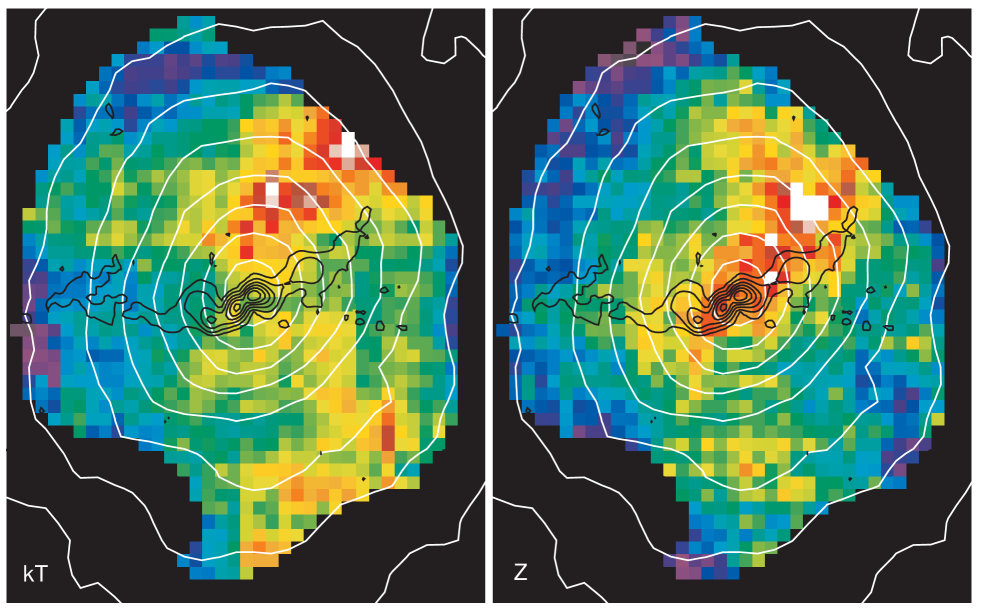
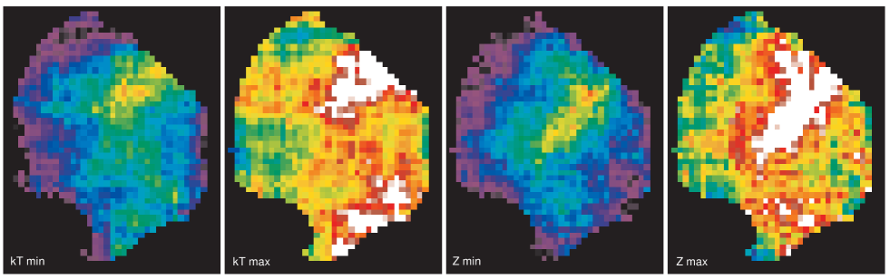
Figure 8: Adaptively binned temperature and abundance maps of AWM 4, based on spectra from all three EPIC instruments. The two upper panels show the best fit values, while the lower panels show the 90% error bounds. Each pixel represents and adaptively chosen square region containing a total of 1600 counts, summed over the three cameras. Pixels for which the (90%) error on the temperature is larger than 20% of the best fit value have been masked out of the images. White contours show X-ray surface brightness, black contours mark VLA-First 20 cm surface brightness. The maps are aligned so that north is toward the top of the page and east is to the left. The pixel size is 6.4^′′. The colour scale in all images is linear. In the temperature maps purple is $\sim$2.2 keV, blue 2.3-2.5, green 2.6-2.7, yellow 2.7-2.8, red 2.9-3.1 and white 3.2 keV and higher. In the abundance maps blue is 0.2-0.4 $Z_{\odot}$, green is 0.5-0.6, red is 0.75-0.95 and white is solar abundance.

	Radii		Map		sas v5.4.1			sas v6.0.0
Region	Inner	Outer	kT	Z	kT	Z	red. $\chi^{2}$/d.o.f.	kT	Z	red. $\chi^{2}$/d.o.f.
	(′′)	(′′)	(keV)	($Z_{\odot}$)	(keV)	($Z_{\odot}$)		(keV)	($Z_{\odot}$)
1	0	120	2.7-3.2	0.35-1.0	2.91${}^{+0.15}_{-0.14}$	$0.69^{+0.13}_{-0.12}$	0.943/283	2.97$\pm$0.16	0.78${}^{+0.17}_{-0.14}$	0.998/269
2	0	120	2.4-3.0	0.3-0.66	2.67$\pm$0.12	0.48${}^{+0.09}_{-0.08}$	1.088/325	2.69$\pm$0.13	0.44${}^{+0.10}_{-0.09}$	1.130/305
3	40	120	2.3-2.7	0.3-0.75	2.46${}^{+0.21}_{-0.18}$	0.44${}^{+0.13}_{-0.10}$	1.048/207	2.64${}^{+0.16}_{-0.15}$	0.51${}^{+0.16}_{-0.11}$	0.984/212
4	14	130	2.6-3.1	0.3-0.8	2.82${}^{+0.13}_{-0.12}$	0.50${}^{+0.10}_{-0.09}$	1.048/328	2.82${}^{+0.14}_{-0.13}$	0.50${}^{+0.10}_{-0.11}$	1.062/309
5	48	95	2.55-2.75	0.5-0.7	2.74${}^{+0.58}_{-0.41}$	0.80${}^{+0.54}_{-0.33}$	1.031/61	2.78${}^{+0.46}_{-0.33}$	0.57${}^{+0.45}_{-0.23}$	0.857/63
6	63	110	2.4-2.8	0.4-0.7	2.87${}^{+0.55}_{-0.43}$	0.55${}^{+0.36}_{-0.24}$	0.969/71	2.74${}^{+0.36}_{-0.33}$	0.41${}^{+0.29}_{-0.20}$	0.901/71

Table 5: Best fit parameters for fits to spectra extracted from the regions shown in Figure 9, using sas v5.4.1 and sas v6.0.0. All fits were performed with hydrogen column fixed at the Galactic value, and counts grouped into bins with a minimum of 20 counts. Only energies between 0.5 and 8.0 keV were used in the fits. The maximum and minimum radius of each region from the surface brightness peak are given in columns 2 and 3. Columns 4 and 5 show the approximate range of values seen in the temperature and abundance maps. Columns 6, 7 and 8 show results from fits to spectra extracted using sas v5.4.1 calibration, columns 9, 10 and 11 show results produced using sas v6.0.0. 90 per cent errors are shown for fitted parameters.

In regions 1-4, the fits are well constrained and agree well with the values found in the map. Regions 5 and 6 are less well constrained, and although the best fit temperature and abundance agree with those found in the map to within the margin of error, the agreement is not particularly good. Region 5 has a temperature at the high end of the range found in the map, and a best fit abundance greater than the value found in the map. Region 6 has a similar problem with temperature. However, both of these regions have relatively low numbers of counts, around 500 in each of the MOS cameras. They are also physically small, not much larger than the PSF, and region 5 lies on a PN chip gap. We therefore do not believe that these discrepancies are serious, and consider the spectral maps to be acceptably accurate and reliable.

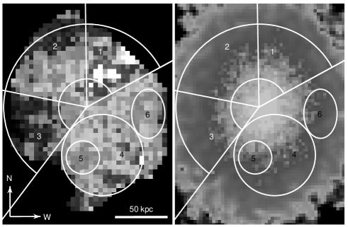
Figure 9: left: Temperature map of the core of AWM 4, as shown in Figure 8. right: Adaptively smoothed mosaiced image of AWM 4, using data from both MOS and PN cameras. Both images show the regions used to extract spectra for comparison between the map spectral fits and those used for the integrated spectra and spectral profiles. Region 4 is a large circle with a smaller circle, region 5, excluded. Further details are given in the text.

As stated in Section 1, we performed our analysis using sas v5.4.1. However, sas v6.0.0 has since been released. A major calibration improvement was incorporated in this release, correcting the telescope vignetting functions of the EPIC instruments. Lumb et al. (2003) demonstrated that the optical axes of the telescopes were not perfectly aligned with their boresights, as had been assumed, meaning that objects apparently on axis were in fact slightly removed from the true axis of the telescopes. As it seems possible that our spectral maps could be altered by this improvement in calibration, we reprocessed the data for AWM 4 using sas v6.0.0, and regenerated the spectral maps. Comparison showed that the improved vignetting correction made little or no difference to the final maps, with the various features appearing unchanged. As a further test, we extracted spectra and responses for the six regions described in the previous paragraph. The results of fits to these spectra are given in Table 5. The fits are all in reasonable agreement with those found for the sas v5 spectra, and with the spectral map. Region 5, which contains the smallest number of counts, has a slightly higher temperature than the map (though with large errors), but the abundance is in better agreement with the map than was the case with the sas v5 spectra. We therefore conclude that while the changes to the vignetting functions may well produce minor changes in the spectral fits to each map pixel, the features observed in the map are likely to be real rather than products of poor calibration.

3.3 Three-dimensional properties

Given the well defined surface brightness profile and near isothermal temperature profile of the cluster, we are able to use our models to estimate some of the 3-d properties of AWM 4. Even the temperature map only shows a 15 per cent variation between the hottest (region 1) and coolest (region 3) areas. We use software provided by S. Helsdon, which uses our surface brightness and temperature models to infer the gas density profile. We use the 2-component surface brightness model shown in Table 3, and assume an isothermal temperature profile with $T$=2.6 keV. This temperature was determined by fitting a constant model to our deprojected temperature profile. Using the projected profile would not affect the choice of $T$ significantly. The density profile is normalised to reproduce the X–ray luminosity of the cluster, determined from our best fitting MEKAL model of the cluster halo. Given this density profile, we can use the well known equation for hydrostatic equilibrium,

$$M_{tot}(<r)=-\frac{kTr}{\mu m_{p}G}\left(\frac{d{\rm ln}\rho_{gas}}{d{\rm ln}r}+\frac{d{\rm ln}T}{d{\rm ln}r}\right),$$ (1)

to calculate the total mass within a given radius. From the gas density and total mass, we can calculate parameters such as gas fraction, cooling time and entropy, where entropy is defined to be

$$S=\frac{T}{n_{e}^{\frac{2}{3}}}.$$ (2)

Errors on the parameters are estimated based on the measured errors in temperature, surface brightness, etc, using a montecarlo technique. We generate 10000 realisations of the profiles and then determine the 1$\sigma$ upper and lower bounds for each parameter at any given radius. Figure 10 shows some of the parameters calculated.

The total mass profile indicates a slightly higher mass than that calculated from the velocity dispersion of the galaxy population (Koranyi & Geller, 2002), but is well within the errors on this optical estimate. Previous mass estimates based on X-ray observations also agree fairly well with our findings. Jones & Forman (1999) and White et al. (1997) estimate the mass based on Einstein data. The former find masses of $\sim$10¹⁴ h^-1$M_{\odot}$ within 0.5 Mpc and 2.6$\times$10¹⁴ h^-1$M_{\odot}$ within 1 Mpc, while the latter find a mass of 1.24$\times$10¹⁴ h^-1$M_{\odot}$ within 1 Mpc. Using ROSAT data, dell’Antonio et al. (1995) find a mass of 5.87$\times$10¹³ h^-1$M_{\odot}$ within 0.42 Mpc. The estimates are quite consistent with each other, at least to within a factor of 2, and also match our gravitating mass profile fairly well. We find a mass of $\sim$9$\times$10¹³ h^-1$M_{\odot}$ within 0.5 Mpc. The gas mass also appears to be quite comparable to other estimates. Jones & Forman (1999) find $M_{gas}$ = (1.95$\pm$0.18)$\times$10¹² h^-2.5$M_{\odot}$ within 0.5 Mpc and (6.71$\pm$0.69)$\times$10¹² h^-2.5$M_{\odot}$ within 1 Mpc, White et al. (1997) estimate $M_{gas}$ = 6.5$\times$10¹² h^-2.5$M_{\odot}$ within 1 Mpc and dell’Antonio et al. (1995) find 3.6$\times$10¹² h^-2.5$M_{\odot}$ within 0.42 Mpc. We find $M_{gas}\simeq$2.5$\times$10¹² h^-2.5$M_{\odot}$ within 0.5 Mpc.

If we assume a virial radius of $\sim$1.2 Mpc (see Section 4.3 for discussion of this choice), the gas fraction at 0.1$\times R_{virial}$ is $\sim$2 per cent, very similar to that found for other systems of similar temperature (Sanderson et al., 2003). The gas fraction at larger radii is somewhat low, but given the extrapolation required to reach the virial radius, both for our data and that used in other studies, some degree of error must be expected. Entropy at 0.1$\times R_{virial}$ is also quite comparable to that found in other systems (Ponman et al., 2003). Following (Pratt & Arnaud, 2003), we have plotted the $S\propto r^{1.1}$ law predicted by numerical modelling of shock heating in a spherical collapse (Tozzi & Norman, 2001) and normalized to the entropy of a 10 keV cluster from Ponman et al. (2003). It is clear that the entropy profile is in close agreement with this prediction, with the profile flattening only within $\sim$0.1 Mpc ($\sim$0.08$\times R_{virial}$). This is very similar to the behaviour reported for A1983 and A1413 by Pratt & Arnaud. However, the cooling time is rather long, 2$\times$10⁹ yr within NGC 6051, a factor of 10 longer than in other relaxed clusters. This suggests that some process has heated the gas or is maintaining its temperature, an issue we will return to in Section 4.

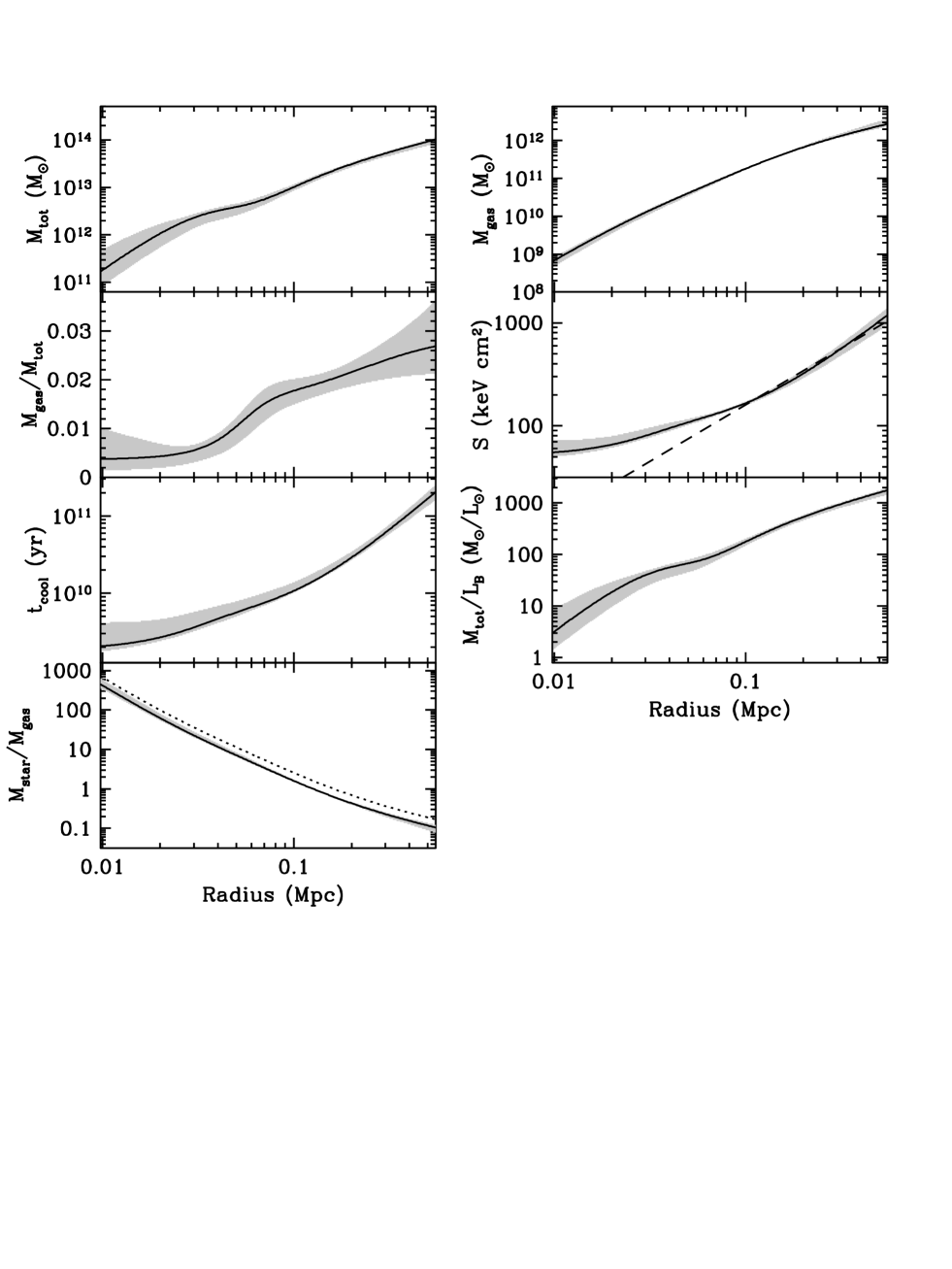
Figure 10: Total mass, gas mass, gas fraction, entropy, cooling time, mass-to-light ratio and stellar mass to gas mass ratio for AWM 4. 1$\sigma$ errors are marked by the grey regions. The profiles are based on data measured to $\sim$160 kpc, but we have extrapolated our models out to 0.5 Mpc. The dashed line in the plot of entropy shows the $S\propto r^{1.1}$ behaviour expected from shock heating. Stellar mass and optical light contributions in the last two plots are from NGC 6051 only. In the stellar mass to gas mass ratio plot, we assume that the mass-to-light ratio of stars in NGC 6051 is either 5 $M_{\odot}/L_{\odot}$ (solid line) or 8 $M_{\odot}/L_{\odot}$ (dotted line). Note that we only include the contribution of NGC 6051 to optical luminosity, so the true mass-to-light ratio of the cluster probably never exceeds 200 $M_{\odot}/L_{\odot}$. Errors are plotted for a stellar mass-to-light ratio of 5 only, so as to avoid confusion.

3.4 Metal masses and supernova enrichment

Given the abundances measured in Section 3.2 and the gas mass profile calculated in Section 3.3, we can estimate the masses of different elements in the intra-cluster medium (ICM). We use our best fitting APEC model of the cluster as a whole and the MEKAL fits to the six radial bins shown in Figure 7. The resulting masses are given in Table 6.

Spectral	Mass ($M_{\odot}$)
Bin	Fe	Si	S	O
Total	8.03$\times$106	9.54$\times$106	2.07$\times$106	7.38$\times$107
1	1.02$\times$105	1.55$\times$105	-	-
2	4.68$\times$105	4.56$\times$105	-	-
3	6.28$\times$105	5.87$\times$105	-	-
4	8.56$\times$105	1.33$\times$106	-	-
5	1.50$\times$106	1.03$\times$106	-	-
6	2.75$\times$106	3.72$\times$106	-	-

Table 6: Mass (in solar units) of Fe, Si, S and O for our best fitting spectral model of the cluster, and for six radial bins. Bin 1 is in the cluster centre, bin 6 is the outermost.

We can also use these masses to estimate the numbers of SNIa and SNII needed to enrich the ICM. We assume yields of Si and Fe for type II supernovae of y_Fe=0.07$M_{\odot}$ and y_Si=0.133$M_{\odot}$ (Finoguenov et al., 2000), and from type Ia supernovae y_Fe=0.744$M_{\odot}$ and y_Si=0.158$M_{\odot}$ (Thielemann et al., 1993). For the cluster as a whole, out to a radius of 260 kpc, we estimate that $\sim$42% of the Fe and $\sim$7% of the Si in the halo was injected by type Ia supernovae. In general the spectral profile suggests that SNIa dominate Fe production in the inner part of the cluster, with $\sim$55-57% of the Fe in bins 2 and 3 being produced by SNIa while 20-30% of the Fe in bins 5 and 6 is produced by this type of supernova. However, the high Si value found for the central bin reverses this trend, suggesting that only $\sim$22% of Fe in this bin was produced in SNIa. We note that the large errors on the Si abundance in this bin make the result somewhat uncertain, however, and that the innermost spectrum is poorly fit with a single temperature model, making the derived abundances less certain. It is therefore likely that the abundances in this bin are in fact compatible with a relatively high fraction of type Ia supernovae.

It has been suggested that more complex models of supernova enrichment, involving two (or more) types of SNIa and revised elemental yields for SNII (e.g., Finoguenov et al., 2002), can produce a more accurate picture of the enrichment history of groups and clusters. In AWM 4, it is notable that the total mass of O and S for the system do not fit into the simple scheme of enrichment presented above, and would suggest a different ratio of supernovae types if we were to use them instead of Si. However, attempts to fit all four elements simultaneously using models including multiple types of SNIa were not successful, primarily because of the large mass of O. This may indicate that the masses derived from the integrated spectrum are not accurate, which would not be surprising given the variation in abundance with radius. We believe that the abundances measured in radial bins are a more accurate measure of the true abundance, but unfortunately the spectra from these bins do not support measurement of more elements, restricting us to the simple supernova models discussed above.

4 Discussion

4.1 Temperature and Abundance structure

The fits presented in Section 3.2 show that the inner $\sim$150 kpc of AWM 4 are relatively isothermal, with a mean temperature of $\sim$2.5 keV. There is a possible slight rise in temperature toward the core of the group, but the trend for increasing abundance toward the center is much stronger. Metallicity rises from 0.3 $Z_{\odot}$ at 150 kpc to $\sim$0.7 $Z_{\odot}$ in the inner parts of NGC 6051. However, these fits use spectra integrated over relatively large areas. The spectral maps shown in Section 3.2.2 use spectra extracted from rather smaller regions, and show considerably more structure than the azimuthally averaged radial spectral profiles. The errors bounds on the values in the maps, and the fits we carried out to check the accuracy of the maps, suggest that much of this structure is real and significant. This does not indicate that the radial profiles are incorrect, but shows the effect of azimuthal averaging on the spectra. The spectral maps correspond to the four inner bins of the radial profiles, and the error bounds on the values in each bin are quite comparable to the range of temperatures and abundances seen in the maps. It is clear though that without the maps we would miss some important structure in the cluster.

The regions shown in Figure 9 were chosen to include some of the features which are visible in the spectral maps. These can be describes as follows. Region 1 contains the high temperature and high metallicity emission which extends to the northwest of the cluster core. Both temperature and abundance show “ridges” of high values, but the peak of the two ridges does not coincide; the highest abundance region runs from the core of NGC 6051 to the northwest, while the peak temperature runs parallel to it but slightly further north, and does not enter the galaxy core. Region 3 is somewhat cooler than most of the rest of the map, and lies to the east of the core, along the line of the eastern radio jet. Region 2 lies to the north of the core, between regions 1 and 3, and has fairly average temperature and abundance. Region 4 covers the area south of the core, and contains some areas of high temperature and moderate abundance. In the eastern part of region 4, we have separated out a smaller region (5) where the temperature is quite low. Region 6 is an area of moderate to low temperature and abundance to the west of the core.

Regions 5 and 6 both have considerably poorer statistics than the other four regions, as they are smaller and contain fewer counts. Region 5 in fact lies over a chip gap in the PN camera, which reduces the number of available counts considerably. This lack of counts in the PN may be at least partially responsible for the cool feature which region 5 was chosen to highlight, and the rather large errors suggest that the feature should be treated with some caution. However, region 6 does not contain chip gaps or regions removed because of point source emission and although the temperature errors for the fit to this region are comparable to those for region 5, the abundance error is slightly smaller. We therefore consider region 6 to be reliably fitted.

4.1.1 Interaction of the radio jets with the ICM

The three main features of the map are the high temperature/abundance areas in region 1, the low temperatures in region 3 and the moderate/high abundances in region 4. Regions 1 and 2 appear to be correlated with the position of the radio jets originating from NGC 6051. To the east, the radio jets points toward and extends into the cool gas of region 3. To the west, the jet extends along the southern boundary of region 1, coincident with the edge of the ridge of high abundance and slightly to the south of the highest temperatures. One explanation of these features are that they are caused by the interaction of the radio jets with the X-ray emitting plasma of the cluster halo.

Chandra observations of massive clusters which contain powerful radio sources have shown that the interaction between jets and surrounding gas can be powerful and complex. Perhaps the best cases are the Perseus cluster (Fabian et al., 2002) and M87 in the Virgo cluster (Young et al., 2002). In Perseus, the radio emission from the radio jets corresponds with areas of low X-ray emission in the inner halo. These are thought to be cavities in the X-ray plasma hollowed out by the pressure of the radio-emitting plasma from the AGN jets. The X-ray gas at the edges of the cavities is cool, indicating that the expansion of the bubble of radio plasma inside has not been rapid enough to cause strong shocks. However, very deep imaging shows density waves in the ICM which are likely to be mild shocks and sound waves caused by the creation of the cavities (Fabian et al., 2003). In M87, cavities are again visible to some extent, but X-ray emission is also enhanced along the radio jets and at the hot spots in the radio lobes. Numerous other features visible in the radio emission correspond to bright areas in the X-ray, again suggesting that the radio plasma can locally compress the ICM, raising its emissivity and surface brightness.

In AWM 4, the cavities seen in more massive clusters may provide an explanation for the cool feature in region 3. The eastern radio jet may have created a cavity in the X-ray halo. If so, the hotter gas which would usually occupy this region would have been displaced, so that we see only the slightly cooler gas in front of and behind it. We see no sign of such a cavity in the X-ray images of the cluster, nor in the residual images which result from subtracting our best fitting surface brightness models from this image. However, the density and (line of sight) depth of the ICM in AWM 4 is considerably smaller than in massive clusters such as Perseus and Virgo, and so we might expect such a cavity to stand out less clearly. AWM 4 is also more distant, the radio source in NGC 6051 is less powerful and we are using a relatively short XMM-Newton observation, with poorer spatial resolution than is available from Chandra, all factors which would make such a feature more difficult to detect. Another possibility is that region 3 is cooler because it contains cool gas drawn out from the galaxy core by the action of the jets, as has been suggested for the regions around the jets of M87 (Böhringer et al., 2001), but the average to low abundance measured in this region argues against this.

The western radio jet might be responsible for the high temperatures in region 1, if it is capable of heating the gas through strong shocks. In order to estimate the shock strength required, we use the standard Rankine-Hugoniot jump conditions (e.g., Landau & Lifshitz, 1959) to estimate the Mach number of the shock from the temperature difference between shocked and unshocked gas. Regions 6 and 2 seem to be relatively unaffected by the radio source, so either could be used to give the temperature of the unshocked plasma. However, as well as being small, region 6 is where we would expect to see a cavity if the radio source was symmetrical, so we have chosen to use region 2. The temperature difference between regions 1 and 2 (0.24 keV) could be produced by a shock of Mach number $\mathcal{M}=1.09$. This would correspond to a density increase across the shock front of a factor of $\sim$1.2, and a corresponding increase in X-ray surface brightness of $\sim$1.4. As the cluster halo is elliptical, with its major axis running roughly north-south, this change is less obvious than it would be if there were a shock front extending due west or east. We estimate that the surface brightness difference between regions 1 and 2 owing to the shape of the halo is a factor of $\sim$1.15, so the increase from any shock will be only marginally above this. We do in fact see a difference between the two regions of a factor of 1.2, and the error associated with the estimate is large enough that we cannot be certain that the gas has been shock heated. It should also be noted that if the shock is not moving in the plane of the sky (i.e. the radio jet does not lie in this plane) then our estimate of the expected change in surface brightness should be lowered. We calculate that an angle of only 15${}^{\hbox{${}^{\circ}$}}$ would be sufficient to make the density jump indistinguishable from that observed.

There are problems with the hypothesis of a shock. The most important is that we do not see any evidence of such a shock to the east, in or around region 3. As we have already mentioned, the interaction of jets with the ICM of more massive clusters does not seem to be accompanied by shock heating, so if this is occurring in AWM 4 it would be an interesting case for further investigation. Similarly, shock heating would not provide an obvious explanation of the high abundances seen along the northern edge of the western jet. The northern jet of Centaurus A has been shown to intersect an Hi cloud, compressing the gas and triggering star formation (Graham, 1998). A degree of star formation in the ICM of AWM 4 could in principle inject metals into the gas through supernovae and stellar winds, but given the observed abundances (as high as solar) it seems unlikely that sufficient numbers of stars could be formed without being detected in the optical.

4.1.2 Movement in the plane of the sky

One further possibility which should be considered is that either NGC 6051 or other galaxies in the cluster have a significant velocity in the plane of the sky. From the relative velocities of the galaxies in the line of sight, the cluster appears to be relaxed, and the recession velocity of NGC 6051 agrees well with the mean velocity of the cluster. However, the cluster is quite extended to both north and south, so it is possible that galaxies might have significant velocities which we cannot measure. If so, a galaxy moving through the cluster core at relatively high speeds might create a gaseous wake through either ram-pressure (Gunn & Gott, 1972) or viscous stripping (Nulsen, 1982). A galaxy moving on a near-radial orbit from south to north or northwest might produce features which would pass through regions 4 and 1. We would expect such a wake to have high abundance, as the gas would have been enriched by stellar winds and supernovae in the galaxy. We would also expect the gas to be relatively cool, as even in early-type galaxies with X-ray emitting halos, temperatures greatly in excess of 1 keV are rare (Brown & Bregman, 1998; Matsushita et al., 2000). This is a problem, as we observe temperatures of 2.5 keV and above, in general hotter than the surrounding medium. Alternatively, NGC 6051 could be moving, a possibility which is supported by the angle between the radio jets. Movement of the galaxy to the south or southwest might produce such an angle, as the pressure of the ICM prevents the jet from moving at the same velocity as the galaxy. It is more difficult to imagine what we would expect to observe were this the case, but it seems possible that the hotter gas to the north of the jets could have been shock heated by the jets before the galaxy moved south to its current position. As a final option, we note that if the galaxy were moving southeast instead of south, the high abundance ridge extending from the core to the northwest might be explained as a tail of enriched gas much like that seen in Abell 1795 (Markevitch et al., 2001). In A1795 this gas is cooler than its surroundings, but in AWM 4 it would have been affected by the eastern radio jet, and possibly heated. Movement of NGC 6051 in either direction does not explain the hot gas in region 4, and as we cannot measure movements in the plane of the sky, these possibilities must remain speculative.

4.2 Abundance - comparison with other systems

A number of other groups and poor clusters have been observed with XMM-Newton and have high quality abundance measurements available. The reflection grating spectrometers (RGS) provide the greatest precision in measurement, as individual line strengths can be modeled. However, the EPIC cameras also provide excellent abundance estimates, and allow the variation of metallicity with radius to be measured.

Systems for which high quality EPIC observations are available include NGC 1399 (Buote, 2002) in Fornax, NGC 5044 (Buote et al., 2003a, b) and M87 in the Virgo cluster (Matsushita et al., 2003). All three of these systems differ from AWM 4 in that they show evidence of multi-phase gas in their cores and are best fit by models with at least two temperature components. However, provided their spectra are sufficiently well described by these models (and providing we have accurately modeled our spectra) it is possible to compare the abundances and their trend with radius. Our findings can be summarised as follows; for the integrated spectrum we find that Si is the most abundant element (of those we fit individually), followed by Fe, S and O. All are subsolar, and all but Si have abundances $<$0.5$Z_{\odot}$. Radial profiles suggest that abundance increases toward the core of the group.

M87 shows a similar trend with radius, but considerably higher abundances. Si, S and Fe peak at almost twice solar, with Si slightly more abundant than Fe and S. We note that Matsushita et al. (2003) use the abundance ratios of Feldman (1992), which produce slightly higher Fe abundances than those of Anders & Grevesse (1989), which we use. Were the authors to use the Anders & Grevesse abundances, Fe abundance would be reduced with respect to Si, a situation much like that which we observe in AWM 4. O is considerably less abundant, with a peak value of $\sim$0.7$Z_{\odot}$. At radii $<$1^′ the profiles turn over and decrease in the galaxy core. This may be caused by rapid cooling through line emission of gas in the high density environment of the cluster core, which will preferentially remove gas with high abundances. However, at the distance of M87, 1^′$\simeq$4.63 kpc, too small a distance for us to resolve in AWM 4. Alternatively, it may be a product of incorrect abundance estimates, caused by the multiphase nature of the gas in the inner core.

The analysis of NGC 1399 shows it to have very supersolar Fe and Si, with abundances increasing in the galaxy core. Si has a peak value of $\sim$1.7$Z_{\odot}$. Once again, Fe is measured using an abundance ratio which differs from that which we use, but corrected to our standard the peak Fe abundance is $\sim$1.5$Z_{\odot}$. NGC 5044 is much like M87, with Fe and Si showing solar or slightly supersolar peak abundances, and abundance rising to a peak before falling in the core. S has a peak abundance of $\sim$0.8$Z_{\odot}$ and does not drop in the inner bins, and O has a low abundance ($\sim$0.2$Z_{\odot}$) at all radii.

For Iron and Silicon, we can calculate the mass of metals found in each system, allowing a direct comparison. For M87,abundance and gas mass profiles are both based on XMM-Newton analysis (Matsushita et al., 2002, 2003), as are the abundances in the other two systems (Buote, 2002; Buote et al., 2003b). The gas mass profile for NGC 1399 is taken from the ROSAT HRI study of Paolillo et al. (2002), and for NGC 5044 we use a profile based on ROSAT PSPC analysis (Sanderson et al., 2003). All three galaxies have high quality abundance measurements to at least 50 kpc radius, and this is the radius within which we calculate metal masses. Table 7 shows the masses of Fe and Si.

System	Fe mass	Si Mass
	($Z_{\odot}$)	($Z_{\odot}$)
NGC 1399	4.0$\times$105	3.4$\times$105
NGC 5044	1.8$\times$106	1.5$\times$106
M87	2.0$\times$106	2.5$\times$106
AWM 4	1.2$\times$106	1.2$\times$106

Table 7: Mass of Fe and Si within the central 50 kpc of each system.

The most obvious differences between these results and ours is the high abundances found in NGC 5044 and M87, and the low metal masses in NGC 1399. The three galaxies have similar optical luminosities to NGC 6051, suggesting that the stellar component in the core of each system is of comparable mass. This suggests that enrichment of the ICM by supernovae should be similar, yet we find differences of at least a factor of two. One possible explanation could be that in the rich Virgo cluster numerous smaller galaxies have passed through the cluster core and have been stripped of their gas either by ram-pressure or tidal forces. This enriched gas is then left in the surroundings of the dominant galaxy, where we observe it. This seems less likely in the case of NGC 5044, however, as this group is poorer than AWM 4; the group has 9 members (Garcia, 1993) compared to 28 in AWM 4 (Koranyi & Geller, 2002). An alternative is the model suggested by Böhringer et al. (2004) in which, during periods of relative stability, the cluster dominant galaxy builds up its own metal rich ISM and a surrounding region of partially enriched mixed ISM/ICM gas. In this model only cluster mergers disrupt this structure and thoroughly mix the gas, so the degree of enrichment is dependent on the time since the last major merger, and the differences we see between systems would reflect differences in their merger histories. This can also be considered as the age of the cool inner core, as during the periods between mergers gas will radiatively cool and presumably be reheated. This model may well be substantially correct, though our results from AWM 4 suggest that AGN activity may also produce gas mixing (on a smaller scale than cluster mergers), reducing the observed abundance peak in the cluster core.

Another alternative is that the multi-phase gas in the three systems discussed above is a symptom of a cooling flow in which the gas is poorly mixed. If the high abundance gas produced by supernovae and galaxy winds does not mix well but instead remains in small clumps, then the high abundance gas will cool much faster than the gas surrounding it. Morris & Fabian (2003) show that such a model can produce very large abundances in the core, surrounding a small low abundance region in which most of the high abundance gas has cooled out of the X-ray regime. In AWM 4, the action of the AGN might have prevented such cooling by reheating gas in the core, or by acting to mix the gas more thoroughly. However, we note that this model is not supported by detailed modeling of EPIC and RGS spectra (Peterson et al., 2003; Kaastra et al., 2004). A final possibility is that the AGN in NGC 6051 is sufficiently effective in mixing the gas that even without abundance inhomogeneities it has suppressed the abundance gradient in the cluster core. Models of rising bubbles (designed to study the interaction of AGN and ICM around M87) Churazov et al., 2001) suggest that the movement of bubbles out through the halo can entrain material and draw it out from the core regions to larger radii. Entrained gas will likely fall back into the core, as it is denser than the surrounding material, but this might offer opportunities for mixing the gas and suppressing the abundance gradient. The strongest argument against this possibility is the abundance gradient in M87. The interaction between radio jets and ICM in that system is clear, but the abundance gradient is still strong, arguing that the gas does not mix. Clearly more detailed modeling of the processes of heating and gas motions produced by AGN activity is required before these issues can be explored further.

4.3 Comparison with MKW 4

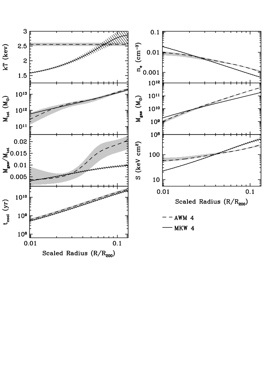
Figure 11: Profiles of X-ray temperature, density, total mass, gas mass, gas fraction, entropy and cooling time for AWM 4 and MKW 4, using data from this paper and O’Sullivan et al. (2003). The profiles are normalised to $R_{\mathrm{200}}$ to correct for the differing masses and sizes of the two clusters. AWM 4 is marked by a dashed line, with the 1$\sigma$ error region marked in grey. MKW 4 is marked by a solid line, with the error region hatched. On some plots the 1$\sigma$ errors are smaller than the line width.

AWM 4 contrasts markedly with MKW 4, a poor cluster of similar mass also recently observed by XMM-Newton (O’Sullivan et al., 2003) and Chandra (Fukazawa et al., 2004). MKW 4 is relatively cool at large radii, with a temperature of 1.6 keV at 250 kpc (Helsdon & Ponman, 2000). The temperature rises to a peak at 100 kpc, then falls again toward the core, to a central temperature of only $\sim$1.4 keV. Abundance within this cooling region is considerably higher than at comparable radii in AWM 4, up to $\sim$1.4$Z_{\odot}$ within the innermost 20 kpc. The abundance of Si and S in this inner region is well in excess of that of Fe, demonstrating that the gas in the inner core has been enriched by supernovae and has remained undisturbed for some time. MKW 4 is not, however, well described by a steady state cooling flow model. Spectral fitting using the EPIC instruments suggests that there is little or no gas at low temperatures, and the RGS data suggests a minimum temperature of $\sim$0.5 keV.

Although the general trend of the temperature profile in MKW 4 seems clear, there is some discrepancy between results for the peak temperature. Our XMM-Newton analysis in a previous paper (O’Sullivan et al., 2003) suggests a peak temperature of $\sim$3 keV. This is in reasonable agreement with results from a ROSAT observation (Helsdon & Ponman, 2000), which found the temperature to be $\sim$2.4 keV at $\sim$45-80 kpc, and poorly defined but above 3 keV at $\sim$80-125 kpc. However, results from ASCA (Finoguenov et al., 2000) contradict these, and the analysis of XMM and Chandra data by Fukazawa et al. (2004) finds a peak temperature of only $\sim$2 keV. One possible explanation of for this is that the background used in our analysis of the XMM data for MKW 4 was incorrect, causing over-subtraction at low energies and overestimation of temperatures. It also seems possible that the opposite is true of the Fukazawa et al. analysis. We have therefore decided to consider both versions of the temperature profile in our comparison with AWM 4. The model fit to our XMM temperature profile is described in O’Sullivan et al. (2003). We fitted the combined Chandra and XMM-Newton temperature data from Fukazawa et al. with a ’Universal’ temperature profile of the form described by Allen et al. (2001), though not normalized to the R₂₅₀₀ overdensity radius. This fit has an outer temperature of 1.76${}^{+0.07}_{-0.06}$ keV, core temperature of 1.35${}^{+0.03}_{-0.05}$ keV, core radius of 8.68${}^{+0.88}_{-1.72}$ kpc, and slope parameter $\eta$=4.63${}^{+3.28}_{-2.23}$. We note that model produces a flat temperature profile with kT=1.76 keV outside $\sim$35 kpc, and so can be considered a very conservative alternative to our XMM-only model.

Figure 11 shows a comparison of some of the 3-dimensional model properties of the two clusters, based on our XMM analysis. We have scaled the models using the $R_{\mathrm{200}}$ radius of the clusters (the radius within which the average density of the cluster is 200 times the critical density of the universe, equivalent to the virial radius). For MKW 4, we use $R_{\mathrm{200}}$=0.97 $h_{\mathrm{75}}$^-1 Mpc (see O’Sullivan et al., 2003, for a discussion of this value). Sanderson et al. (2003) use ROSAT and ASCA data to estimate $R_{\mathrm{200}}$ for AWM 4, and find $R_{\mathrm{200}}$=1.44${}^{+0.32}_{-0.27}$ $h_{\mathrm{75}}$^-1 Mpc. Extrapolating from our surface brightness models and assuming a constant temperature, we estimate $R_{\mathrm{200}}$=1.18 $h_{\mathrm{75}}$^-1 Mpc, similar to the value we would obtain based on the work of Navarro et al. (1995), who found $R_{\mathrm{200}}$=1.17 $h_{\mathrm{75}}$^-1 Mpc. There are potential problems with using any of these estimates. Estimates based on an isothermal temperature profile will not account for any temperature gradient at larger radii, while the ASCA and ROSAT analysis assumed a central cooling region and therefore may not model the inner halo accurately. However, the estimates are in broad agreement, and we choose to use the estimate based on the XMM-Newton data, noting the inherent uncertainty.

A second comparison, using the Fukazawa et al. temperature profile, produced very similar results. As expected, gas density and gas mass, which are dependent primarily on the surface brightness profile, were essentially unchanged, as was the cooling time. The total mass profile was slightly shallower at large radii, with the mass at the outer boundary of the plot falling by a factor of $\sim$2. The maximum entropy also falls by a factor of $\sim$3, agreeing almost exactly with the entropy calculated for AWM 4. However, neither of these changes significantly alters our understanding of the behaviour of the system. Gas fraction shows the largest change, and we show all three gas fraction profiles in Figure 12. The most obvious change is that when using the Fukazawa et al. temperature profile for MKW 4, gas fraction is found to rise outside 0.04$\times$$R_{\mathrm{200}}$, producing a maximum value of 1.8% compared to $\sim$1% if our temperature profile is used. This brings it into closer agreement with AWM 4, but we note that in both versions of the profile, MKW 4 has a significantly different gas fraction profile from that of AWM 4 between $\sim$0.05 and 0.1$\times$$R_{\mathrm{200}}$. We believe this comparison shows that, with the possible exception of gas fraction, the profiles shown in Figure 11 can be directly compared with confidence in their accuracy. We therefore proceed with this comparison, but exercise caution regarding the results for gas fraction.

Several important differences in the structure of the two clusters can be seen in the profiles. MKW 4 has a steeper gas density profile than AWM 4 (at least over the range covered by these models), with a larger mass of gas within $\sim$0.02$\times$$R_{\mathrm{200}}$. It also has a higher total mass in the core, though the total mass profiles at larger radii are quite similar. The gas in the inner region has a significantly shorter cooling time and lower entropy than is seen in AWM 4. The gas fraction profile suggests that while the two clusters have comparable gas fractions within $\sim$0.03$\times$$R_{\mathrm{200}}$, in AWM 4 the rise in gas fraction outside this radius is steeper than in MKW 4, and that AWM 4 may have a considerably higher gas fraction than MKW 4 at large radii. Gas fraction almost certainly rises to match that of AWM 4 outside the radius of our analysis; if the Fukazawa et al. temperature profile is used, the two clusters come into agreement at $\sim$0.2$\times$$R_{\mathrm{200}}$; if our temperature model is used, the turn over in temperature produces a lower gas fraction, but when the profile levels off at larger radii, as the ROSAT results show it does, the fraction will likely rise again.

The similarity in mass outside the core suggests that these two systems are fundamentally quite similar. The difference in mass in the core is most likely caused by the difference in mass of the two dominant ellipticals. Assuming a stellar mass-to-light ratio of 5 $L_{\odot}/M_{\odot}$ NGC 4073, the dominant galaxy of MKW 4, has a mass of 5.12$\times$10¹¹ $M_{\odot}$, compared to 2.88$\times$10¹¹ $M_{\odot}$for NGC 6051. Our X-ray based mass profiles do not exactly match these values estimated from the optical data, but the difference between the two is clear.

The other major differences in the profiles can largely be explained as a consequence of the different temperature profiles of the two clusters. Gas in the core of MKW 4 has been able to cool, leading to the observed low entropy and short cooling time. In comparison, gas in the core of AWM 4 has been heated, lowering the density, flattening the inner entropy profile and “puffing up” the halo. The gas fraction profile suggests that the heating may have effectively moved gas outward, building up a low density core and a steeper density gradient at larger radii. We cannot determine whether AWM 4 may have an inherently higher gas fraction than MKW 4 as we do not have sufficiently deep observations to model the two galaxies out to their virial radii, but it seems possible that this may be the case to some degree. Alternatively the two could have similar overall gas fractions at large radii, but with MKW 4 having a larger core region in which the gas fraction is low. If the steep rise in the gas fraction profile of AWM 4 is caused by AGN heating and movement of gas outward, this could indicate that the process lasted longer and was more effective in MKW 4. However, as we cannot discriminate between these possibilities with the data available, we restrict ourselves to the conclusion that the combination of cooling in MKW 4, heating in AWM 4 and the difference in central galaxy mass produces the differences in core gas mass and density.

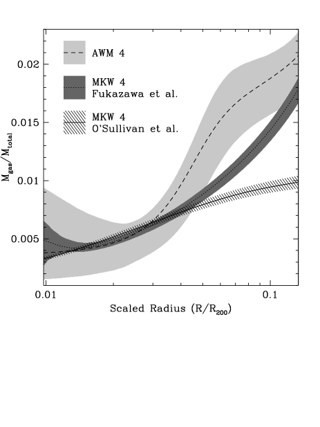
Figure 12: Gas fraction profiles for AWM 4 and MKW 4. The MKW 4 profiles were determined using model fits to either the Fukazawa et al. (2004) XMM+Chandra temperature profile or the O’Sullivan et al. (2003) XMM-only profile, which has a higher peak temperature.

MKW 4 is probably still in the process of developing a cooling flow, as it does not yet show any sign of gas cooler than 0.5 keV. If the gas was hotter in the past, the most likely source of heating is an AGN in NGC 4073, which has since become quiescent. If this is the case, then the differences we see between the two clusters are largely the product of the AGN activity in their dominant galaxies; it happens that we are observing them at different phases of their duty cycle. In NGC 6051 the AGN has been active for some time and has heating the surrounding ICM, in the process probably removing its own fuel source. In NGC 4073, we see the opposite, with the AGN quiescent for a long period and perhaps soon to reactivate as cooling provides it with material to accrete. This is a fine example of the influence of the ICM on the cluster dominant galaxy and vice versa.

We can estimate the energy output required to produce the isothermal profile observed in AWM 4, assuming that it once had a temperature profile such as that seen in MKW 4. The total energy required is $\sim$9$\times$10⁵⁸ erg. If the AGN has an active period of 100 Myr, this means that a power output of $\sim$3$\times$10⁴³ $\mbox{~{}erg}\mbox{~{}s}^{-1}$ is required. Böhringer et al. (2002) estimate the kinetic energy output of the AGN in M87, NGC 1275 and Hydra A to be in the range 1.2$\times$10⁴⁴-2$\times$10⁴⁵ $\mbox{~{}erg}\mbox{~{}s}^{-1}$ based on the bubbles visible in the ICM of these clusters (see also McNamara et al., 2000; Nulsen et al., 2002). We have estimated the current power output of the AGN in NGC 6051 from the flux detected from the radio emission in and around NGC 6051. Radio fluxes have been measured between 26.3 MHz and 10.55 GHz (Neumann et al., 1994; Wright & Otrupcek, 1990; Viner & Erickson, 1975), and from these we calculate a spectral index of -0.9$\pm$0.05, fairly typical for an FR-I radio galaxy. We estimate the power in this frequency range to be $\sim$9.4$\times$10⁴⁰ $\mbox{~{}erg}\mbox{~{}s}^{-1}$. However, as Fabian et al. (2002) demonstrate for 3C 84 in the Perseus cluster, this can only be considered a lower limit on the actual jet power. Based on the cavities observed in the Perseus cluster core, it is estimated that the power of the jets is 10^44-45 $\mbox{~{}erg}\mbox{~{}s}^{-1}$, compared to a total emission in the radio band of 10^40-41 $\mbox{~{}erg}\mbox{~{}s}^{-1}$. Our system is less powerful and we do not see cavities in the X-ray emission, but is seems reasonable to expect the jet power to be at least$\sim$10⁴³ $\mbox{~{}erg}\mbox{~{}s}^{-1}$.

There are numerous other suggested sources of heating in galaxy clusters, including star formation and galaxy winds, conduction of heat inward from the outer halo, shock heating during the merger of a sub-cluster, and AGN activity. In the case of AWM 4, the first three of these can be dismissed relatively quickly. Conduction can certainly be ruled out, as the deprojected temperature profile shows an increasing temperature toward the core. A recent merger is equally unlikely, as the cluster is relaxed with no strong substructure. Similarly, there is little evidence of recent star formation in the central galaxy, and to provide the energy necessary to heat the halo, star formation would have had to have been extensive and powerful. Given the strong extended radio source hosted within NGC 6051, it seems clear that AGN heating is the most likely cause of the roughly isothermal temperature profile we observe.

5 Summary and Conclusions

AWM 4 is at first glance a good example of a relaxed cluster, with no significant substructure visible in X-ray images of its halo. Spectral fitting shows that the cluster core is reasonably well described by a single temperature plasma model with kT=2.5-2.6 keV and abundance $\sim$0.5$Z_{\odot}$. Radial spectral profiles show that the cluster is close to isothermal out to a radius of $\sim$160 kpc. Abundance rises from $\sim$0.3$Z_{\odot}$ at 160 kpc to $\sim$0.7$Z_{\odot}$ in the cluster core. The highest abundances coincide with the position of NGC 6051 and are presumably the product of enrichment by supernovae within this galaxy.

Our XMM-Newton analysis has revealed some new aspects to the cluster, many of which appear to be related to the powerful AGN hosted by NGC 6051. The abundances we observe for the cluster are rather low compared to other systems which have been observed by XMM-Newton. Possible explanations of this include mixing of the cluster gas, driven by the activity of the AGN. Spectral mapping of the cluster reveals a number of features whose abundances and temperatures diverge from the mean values for the cluster. The eastern radio jet of 4C+24.36 coincides with a region of low temperatures which may indicate a cavity in the cluster X-ray halo. The western jet coincides with the southern edge of a region of high abundance and high temperature. The high temperatures may be caused by shock heating of the gas caused as the radio jet compresses the X-ray plasma. However, the high abundances are more difficult to explain, as is a region of enhanced temperature and abundance to the south of the galaxy core. These may indicate enrichment of the ICM through stripping of galaxies in the cluster, possibly including NGC 6051. The velocity dispersion of the galaxies in the cluster does not indicate any substructure or outlying members, but the cluster is elongated along a north-south axis and the radio source, which appears to have a wide angle tail structure, suggests motion. Unfortunately we cannot determine motions in the plane of the sky.

Using the best fitting surface brightness profile of the cluster and assuming it to be approximately isothermal, we have modeled the three dimensional properties of the cluster X-ray halo and potential well. The gas mass and total gravitating mass we estimate agree with previous estimates, both from older X-ray observations and based on the galaxy population. We find that although the cluster entropy is in the expected range at 0.1$\times$$R_{\mathrm{200}}$, the entropy in the cluster core is somewhat higher than in comparable systems, and the cooling time is long. The gas fraction profile also shows a strong increase at 30-70 kpc. We interpret these factors, in combination with the lack of a cooling core in this apparently relaxed system, as indications that AGN activity has reheated the gas in the cluster core. We estimate the power available from the AGN to be sufficient for this task, and suggest that the current temperature profile and large-scale radio jets indicate that the AGN has been active for some time, and may perhaps be nearing the end of its active period. The lack of ongoing cooling implies that the fuel available for the AGN must soon run out, leading to dormancy and the reestablishment of cooling in the inner cluster halo.

Acknowledgments
We are very grateful to S. Helsdon for the use of his 3-d gas properties software, and to the referee, Alexis Finoguenov, for a thorough reading of the paper and numerous useful suggestions. We would also like to thank A. Read and B. Maughan for their advice on XMM analysis, and the use of their software. The authors made use of the NASA and Lyon Extragalactic Databases, and were supported in part by NASA grants NAG5-10071 and GO2-3186X.

References

- Albert et al. (1977) Albert C. E., White R. A., Morgan W. W., 1977, ApJ, 211, 309
- Allen et al. (2001) Allen S. W., Schmidt R. W., Fabian A. C., 2001, MNRAS, 328, L37
- Anders & Grevesse (1989) Anders E., Grevesse N., 1989, Geo. et Cosmo. Acta, 53, 197
- Arnaud et al. (2002) Arnaud M., Majerowicz S., Lumb D., Neumann D. M., Aghanim N., Blanchard A., Boer M., Burke D. J., Collins C. A., Giard M., Nevalainen J., Nichol R. C., Romer A. K., Sadat R., 2002, A&A, 390, 27
- Böhringer et al. (2001) Böhringer H., Belsole E., Kennea J., Matsushita K., Molendi S., Worrall D. M., Mushotzky R. F., Ehle M., Guainazzi M., Sakelliou I., Stewart G., Vestrand W. T., Dos Santos S., 2001, A&A, 365, L181
- Böhringer et al. (2004) Böhringer H., Matsushita K., Churazov E., Finoguenov A., Ikebe Y., 2004, A&A, 416, L21
- Böhringer et al. (2002) Böhringer H., Matsushita K., Churazov E., Ikebe Y., Chen Y., 2002, A&A, 382, 804
- Brown & Bregman (1998) Brown B., Bregman J., 1998, ApJ, 495, L75
- Buote (2002) Buote D. A., 2002, ApJ, 574, L135
- Buote et al. (2003a) Buote D. A., Lewis A. D., Brighenti F., Mathews W. G., 2003a, ApJ, 594, 741
- Buote et al. (2003b) Buote D. A., Lewis A. D., Brighenti F., Mathews W. G., 2003b, ApJ, 595, 151
- Cash (1979) Cash W., 1979, ApJ, 228, 939
- Churazov et al. (2001) Churazov E., Brüggen M., Kaiser C. R., Böhringer H., Forman W., 2001, ApJ, 554, 261
- dell’Antonio et al. (1995) dell’Antonio I. P., Geller M. J., Fabricant D. G., 1995, AJ, 110, 502
- Fabian et al. (2002) Fabian A. C., Celotti A., Blundell K. M., Kassim N. E., Perley R. A., 2002, MNRAS, 331, 369
- Fabian et al. (2003) Fabian A. C., Sanders J. S., Allen S. W., Crawford C. S., Iwasawa K., Johnstone R. M., Schmidt R. W., Taylor G. B., 2003, MNRAS, 344, L43
- Fabian et al. (2000) Fabian A. C., Sanders J. S., Ettori S., Taylor G. B., Allen S. W., Crawford C. S., Iwasawa K., Johnstone R. M., Ogle P. M., 2000, MNRAS, 318, L65
- Feldman (1992) Feldman U., 1992, Physica Scripta, 46, 202
- Finoguenov et al. (2001) Finoguenov A., Arnaud M., David L. P., 2001, ApJ, 555, 191
- Finoguenov et al. (2000) Finoguenov A., David L. P., Ponman T. J., 2000, ApJ, 544, 188
- Finoguenov et al. (2002) Finoguenov A., Matsushita K., Böhringer H., Ikebe Y., Arnaud M., 2002, A&A, 381, 21
- Fukazawa et al. (2004) Fukazawa Y., Kawano N., Kawashima K., 2004, ApJ, 606, L109
- Fukazawa et al. (1998) Fukazawa Y., Makishima K., Tamura T., Ezawa H., Xu H., Ikebe Y., Kikuchi K., Ohashi T., 1998, PASJ, 50, 187
- Garcia (1993) Garcia A. M., 1993, A&AS, 100, 47
- Graham (1998) Graham J. A., 1998, ApJ, 502, 245
- Grevesse & Sauval (1998) Grevesse N., Sauval A. J., 1998, Space Sci. Rev., 85, 161
- Gunn & Gott (1972) Gunn J. E., Gott J. R. I., 1972, ApJ, 176, 1
- Helsdon & Ponman (2000) Helsdon S. F., Ponman T. J., 2000, MNRAS, 315, 356
- Houck & Denicola (2000) Houck J. C., Denicola L. A., 2000, in ASP Conf. Ser. 216: Astronomical Data Analysis Software and Systems IX ISIS: An Interactive Spectral Interpretation System for High Resolution X-Ray Spectroscopy. ASP, San Francisco, p. 591
- Jansen et al. (2001) Jansen F., Lumb D., Altieri B., Clavel J., Ehle M., Erd C., Gabriel C., Guainazzi M., Gondoin P., Much R., Munoz R., Santos M., Schartel N., Texier D., Vacanti G., 2001, A&A, 365, L1
- Jones & Forman (1999) Jones C., Forman W., 1999, ApJ, 511, 65
- Kaastra & Mewe (1993) Kaastra J., Mewe R., 1993, A&AS, 97, 443
- Kaastra et al. (2004) Kaastra J. S., Tamura T., Peterson J. R., Bleeker J. A. M., Ferrigno C., Khan S. M., Paerels F. B. S., Piffaretti R., Branduardi-Raymont G., Böhringer H., 2004, A&A, 413, 415
- Koranyi & Geller (2002) Koranyi D. M., Geller M. J., 2002, AJ, 123, 100
- Kriss et al. (1983) Kriss G. A., Cioffi D. F., Canizares C. R., 1983, ApJ, 272, 439
- Landau & Lifshitz (1959) Landau L., Lifshitz E., 1959, Fluid mechanics. Oxford: Pergamon Press
- Liedahl et al. (1995) Liedahl D. A., Osterheld A. L., Goldstein W. H., 1995, ApJ, 438, L115
- Lumb et al. (2003) Lumb D. H., Finoguenov A., Saxton R., Aschenbach B., Gondoin P., Kirsch M., Stewart I. M., 2003, Experimental Astronomy, 15, 89
- Markevitch et al. (2001) Markevitch M., Vikhlinin A., Mazzotta P., 2001, ApJ, 562, L153
- Marty et al. (2002) Marty P. B., Kneib J. P., Sadat R., Ebeling H., Smail I., 2002, proc. SPIE, 4851, 208
- Matsushita et al. (2002) Matsushita K., Belsole E., Finoguenov A., Böhringer H., 2002, A&A, 386, 77
- Matsushita et al. (2003) Matsushita K., Finoguenov A., Böhringer H., 2003, A&A, 401, 443
- Matsushita et al. (2000) Matsushita K., Ohashi T., Makishima K., 2000, PASJ, 52, 685
- McNamara et al. (2000) McNamara B. R., Wise M., Nulsen P. E. J., David L. P., Sarazin C. L., Bautz M., Markevitch M., Vikhlinin A., Forman W. R., Jones C., Harris D. E., 2000, ApJ, 534, L135
- Morris & Fabian (2003) Morris R. G., Fabian A. C., 2003, MNRAS, 338, 824
- Navarro et al. (1995) Navarro J. F., Frenk C. S., White S. D. M., 1995, MNRAS, 275, 720
- Neumann et al. (1994) Neumann M., Reich W., Fuerst E., Brinkmann W., Reich P., Siebert J., Wielebinski R., Truemper J., 1994, A&AS, 106, 303
- Nulsen (1982) Nulsen P. E. J., 1982, MNRAS, 198, 1007
- Nulsen et al. (2002) Nulsen P. E. J., David L. P., McNamara B. R., Jones C., Forman W. R., Wise M., 2002, ApJ, 568, 163
- O’Sullivan et al. (2003) O’Sullivan E., Vrtilek J. M., Read A. M., David L. P., Ponman T. J., 2003, MNRAS, 346, 525
- Paolillo et al. (2002) Paolillo M., Fabbiano G., Peres G., Kim D.-W., 2002, ApJ, 565, 883
- Peterson et al. (2003) Peterson J. R., Kahn S. M., Paerels F. B. S., Kaastra J. S., Tamura T., Bleeker J. A. M., Ferrigno C., Jernigan J. G., 2003, ApJ, 590, 207
- Ponman et al. (2003) Ponman T. J., Sanderson A. J. R., Finoguenov A., 2003, MNRAS, 343, 331
- Pratt & Arnaud (2003) Pratt G. W., Arnaud M., 2003, A&A, 408, 1
- Pratt et al. (2001) Pratt G. W., Arnaud M., Aghanim N., 2001, in Neumann D. M., Tranh Thanh Van J., eds, Clusters of Galaxies and the High Redshift Universe Observed in X-rays: XMM-Newton observations of galaxy clusters; the radial temperature profile of A2163. p. in press
- Read & Ponman (2003) Read A. M., Ponman T. J., 2003, A&A, 409, 395
- Sanderson et al. (2003) Sanderson A. J. R., Ponman T. J., Finoguenov A., Lloyd-Davies E. J., Markevitch M., 2003, MNRAS, 340, 989
- Schombert (1987) Schombert J. M., 1987, ApJS, 64, 643
- Smith et al. (2001) Smith R. K., Brickhouse N. S., Liedahl D. A., Raymond J. C., 2001, ApJ, 556, L91
- Thielemann et al. (1993) Thielemann F.-K., Nomoto K., Hashimoto M., 1993, in Prantzos N., Vangioni-Flam E., Casse M., eds, , Origin and Evolution of the Elements. Cambridge Univ. Press
- Tozzi & Norman (2001) Tozzi P., Norman C., 2001, ApJ, 546, 63
- Véron-Cetty & Véron (2001) Véron-Cetty M.-P., Véron P., 2001, A&A, 374, 92
- Valentijn & Giovanelli (1982) Valentijn E. A., Giovanelli R., 1982, A&A, 114, 208
- Viner & Erickson (1975) Viner M. R., Erickson W. C., 1975, AJ, 80, 931
- White et al. (1997) White D. A., Jones C., Forman W., 1997, MNRAS, 292, 419
- Wright & Otrupcek (1990) Wright A., Otrupcek R., 1990, in PKS Catalog (1990) Parkes Catalog, 1990, Australia telescope national facility.. p. 0
- Young et al. (2002) Young A. J., Wilson A. S., Mundell C. G., 2002, ApJ, 579, 560