HI Narrow Self–Absorption in Dark Clouds: Correlations with Molecular Gas and Implications for Cloud Evolution and Star Formation

Abstract

We present the results of a comparative study of HI narrow self–absorption (HINSA), OH, ¹³CO, and C¹⁸O in five dark clouds. We find that the HINSA generally follows the distribution of the emission of the carbon monoxide isotopologues, and has a characteristic size close to that of ¹³CO. This confirms earlier work (Li & Goldsmith, 2003) which determined that the HINSA is produced by cold HI which is well mixed with molecular gas in well–shielded regions. The OH and ¹³CO column densities are essentially uncorrelated for the sources other than L1544. Our observations indicate that the central number densities of HI are between 2 and 6 cm^-3, and that the ratio of the hydrogen density to total proton density for these sources is 5 to 27$\times 10^{-4}$. Using cloud temperatures and the density of atomic hydrogen, we set an upper limit to the cosmic ray ionization rate of 10^-16 s^-1. We present an idealized model for HI to H₂ conversion in well–shielded regions, which includes cosmic ray destruction of H₂ and formation of this species on grain surfaces. We include the effect of a distribution of grain sizes, and find that for a MRN distribution, the rate of H₂ formation is increased by a factor of 3.4.

Comparison of observed and modeled fractional HI abundances indicates ages for these clouds, defined as the time since initiation of HI $\rightarrow$ H₂ conversion, to be 10^6.5 to 10⁷ yr. Several effects may make this time a lower limit, but the low values of n_HI we have determined make it certain that the time scale for evolution from a possibly less dense atomic phase to almost entirely molecular phase, must be a minimum of several million years. This clearly sets a lower limit to the overall time scale for the process of star formation and the lifetime of molecular clouds.

1 INTRODUCTION

The study of atomic hydrogen in dense interstellar clouds has a long history. Very early measurements of dark clouds indicated no correlation of atomic hydrogen and dust opacity (Bok, Lawrence, & Menon, 1955). Subsequent measurements in fact showed an anticorrelation between the HI column density and extinction (e.g. Garzoli & Varsavsky, 1966). These pioneering observations of the Taurus region were followed by a broader survey of dust clouds by Heiles (1969) in which a number of spectra showing “fluctuations” were found, but one object showed clear evidence for “self–absorption”: a narrow absorption feature superimposed on a wider emission line. In this source in Taurus, the velocity of the HI self–absorption agreed with that of the OH emission.

Since that time, a number of large–scale and focused studies of HI in dark clouds have been carried out (e.g. Knapp, 1974; Heiles & Gordon, 1975; Wilson & Minn, 1977; McCutcheon, Shuter, & Booth, 1978; Myers et al., 1978; Bowers, Kerr, & Hawarden, 1980; Minn, 1981; Batrla, Wilson, & Rahe, 1981; Shuter, Dickman, & Klatt, 1987; van der Werf, Goss, & Vanden Bout, 1988; Feldt & Wendker, 1993; Montgomery, Bates, & Davies, 1995). With improved sensitivity and higher angular and spectral resolution, most of these studies identify self–absorption features. The inherent ambiguity between a temperature fluctuation in the emitting region and a distinct, colder, foreground source responsible for the absorption makes it difficult to distinguish between these two quite different situations for an arbitrary line of sight (e.g. Gibson, Taylor, Higgs, & Dewdney, 2000; Kavars et al., 2003), and it is still only for relatively nearby clouds that the location of the cold atomic hydrogen can be identified with certainty.

A key element in pinpointing the location of cold HI is its association with molecular emission, and the greatest difference between early and current observations of HI self–absorption is the recognition that optically–identified dust clouds are cold (T $\simeq$ 10 K), dense (n $\geq$ 10³ cm^-3) primarily molecular regions. The availability of reasonably well–understood tracers which are surrogates for the largely–unobservable H₂ means that determining the HI to H₂ abundance ratio in nearby dark clouds is now practical. These regions are of interest in their own right, as they contain the dense cores in which low mass star formation can occur, and in regions such as the Taurus molecular cloud, these are the only regions in which star formation appears to be occurring. Additionally, because the visual extinction of these dark clouds is sufficient to make photodestruction of H₂ unimportant in their central regions, they are ideal laboratories for comparative studies of the atomic and molecular forms of hydrogen under relatively simple conditions.

A recent survey of dark clouds using the Arecibo telescope revealed that over 80% of the clouds in Taurus exhibit HI narrow self–absorption (Li & Goldsmith, 2003), which we gave the acronym HINSA. The atomic hydrogen responsible was shown to be associated with molecular material traced by OH, C¹⁸O  and ¹³CO  on the basis of (1) the agreement in velocities, (2) the close agreement of nonthermal line widths, and (3) the low temperature implied by the depth of the HI features and the small values of the nonthermal contribution to the line width. Mapping data for only one cloud was available, which showed reasonable agreement between the column densities of cold HI, and OH, and the integrated intensity of C¹⁸O.

We have continued and extended this work, and in the present paper report observations of four clouds: L1544, B227, L1574, and CB45. In Section 2 we present the observations of HI absorption, OH, C¹⁸O  ¹³CO  and CI emission. In Section 3, we discuss the spectra and determination of the column densities of the species we have observed. We also present the maps of these tracers in each of the sources. In Section 4 we present and discuss correlations of the column densities of different tracers. In Section 5 we derive the number densities of the species and determine the HI to H₂ ratio for each of the clouds. In Section 6 we present models for the time dependence of the atomic and molecular hydrogen density. Comparison of models and our data allows us to draw conclusions about the lifetime of these clouds in Section 7.

2 OBSERVATIONS

The HI and OH data were obtained using the 305 m radio telescope of the Arecibo Observatory. The data were obtained in four observing sessions between November 2002 and May 2003. The telescope was calibrated as described by Li & Goldsmith (2003) and both the HI and OH data, which were obtained simultaneously using the “L-wide” receiver, have been corrected for the main beam efficiency of 0.60. The elliptical beam has FWHM beam dimensions of 3^′.1 by 3^′.6. We observed using total power “on source” observations only, and removed the receiver noise and system bandpass by fitting a low–order polynomial to the spectrometer output. For these observations, the autocorrelation spectrometer was configured to have three subcorrelators with 1024 lags each covering 0.391 MHz centered on frequencies of the HI, OH(1665 MHz) and OH(1667 MHz) transitions. A fourth subcorrelator with 1024 lags covering a 0.781 MHz bandwidth was centered on the HI line, and was used for removing the instrumental baseline when wider emission features were encountered. The nominal channel spacing for the HI observations was 0.08 km s^-1, but data were typically smoothed to a velocity resolution of 0.16 km s^-1.

The receiver temperature was typically 30 K at 1420, 1665, and 1667 MHz, but the total system temperature was more than double this value when observing 21–cm emission lines. The integration time per position was 1 minute. This was sufficient to give good signal to noise for the HI absorption features, and also satisfactory OH 1667 MHz emission spectra.

Observations of ¹²CO, ¹³CO, and C¹⁸O were obtained using the Five College Radio Astronomy Observatory 13.7 m radio telescope , during April and May 2003 and January 2004. The 32 pixel Sequoia receiver was configured to observe ¹³CO and C¹⁸O simultaneously for most of the data taking. The autocorrelation spectrometer for each isotopologue had a bandwidth of 25 MHz and 1024 lags, corresponding to a channel spacing in velocity of 0.067 km s^-1at 110 GHz. We mapped each source using “on the fly” data taking, covering a region determined by the HI observations obtained previously. The angular size of the maps ranged from 12^′ to 27^′. System temperatures were typically 200 K for ¹³CO and C¹⁸O  and 450 K for ¹²CO. The integration time per sample point was nominally 10 s. The oversampled data was convolved to a circular Gaussian having the same solid angle as the Arecibo beam, corresponding to a FWHM equal to 3.3 ^′. We smoothed the data in velocity to the same 0.16 km s^-1 resolution used for the HI and OH. Additional data on ¹²CO for the source L1544 were obtained to be able to make accurate corrections for the optical depth of the ¹³CO emission. All FCRAO data were corrected for appropriate main beam efficiencies, which are 0.49 for ¹³CO and C¹⁸O  and 0.45 for ¹²CO.

We obtained the data on atomic carbon (CI) using the Submillimeter Wave Astronomy Satellite (SWAS; Melnick et al., 2000). Observations having total integration time of 1 hour per position were obtained using position switching to a reference position selected to have very weak or undetectable ¹²CO J$\rightarrow$0 emission. The data have been corrected for the main beam efficiency of 0.90. The SWAS beam size is relatively large (3^′.5 x 5^′.0 at the 492 GHz frequency of the CI line) and combined with low intensities of this transition in dark clouds, we were only partially successful in being able to delineate the distribution of CI relative to that of the other species studied. These results are further discussed in Section 3.

3 COLUMN DENSITIES, SPECTRA, AND DISTRIBUTIONS

Determination of the distances to dark clouds such as those in the present study presents considerable difficulties. L1544 is associated with the Taurus dark cloud, for which the distance given here is the average of various techniques described by Elias (1978). B227 is at a galactic latitude of -0.46^o, and is located in a complex region of considerable extinction. Arquilla (1984) observed the same cloud as studied here, and with a B-V color excess technique, derived a distance of 600 pc but there is obviously a large uncertainty. Tomita, Saito & Ohtani (1979) studied the dark nebula L1570 which is often (e.g. Clemens & Barvainis, 1988) used interchangeably with B227, but there is a difference of over 8^′ between the Arquilla and Tomita et al. positions. The latter authors, using star counts derived a distance 300 pc, but again with significant uncertainty. Earlier, Bok & McCarthy (1974) gave an “adopted” distance of 400 pc for B227. We here adopt a distance of 400 pc. L1574 and CB45 are lumped together by Kawamura et al. (1998) and are assigned the 300 pc distance of the not too distant L1570 determined by Tomita, Saito, & Ohtani (1979), which we adopt here. The source coordinates and distances we have adopted are given in Table 1.

3.1 Cold HI

The column density of the cold, relatively quiescent atomic hydrogen was found by assuming an excitation temperature of 10 K, and solving for the optical depth of the absorbing gas as described in Li & Goldsmith (2003). The maximum values of $\tau_{coldHI}$ are modest, ranging from 0.34 for L1574r to 0.69 for L1574b. As discussed in the earlier paper, the effect of foreground HI is primarily to reduce the apparent value of the 21–cm absorption optical depth. We have corrected the optical depth as described in Li & Goldsmith (2003), with values of p determined from the distances given in Table 1. The correction was less than 15 %. The corrected optical depth and the line width of the gaussian fit to the absorption profile together yield the column density of cold absorbing gas using equation 18 of Li & Goldsmith (2003).

We present the peak main beam temperature T_mb at the positions of maximum emission of each cloud in Table 2. The values given are the peak antenna temperatures divided by the main beam efficiency.

3.2 OH

The OH emission is almost certainly optically thin. The peak main beam temperatures are typically 0.5 K, except in L1544 where the line is a factor of three stronger. The modest A–coefficient (7.8$\times 10^{-11}$ s^-1; Destombes et al., 1977) and typical collisional rate coefficients ($\geq$ 2$\times 10^{-11}$ cm³ s^-1; Dewangan, Flower, & Alexander, 1987; Offer & van Dishoeck, 1994) result in a critical density $\leq$ 4 cm^-3, so that the excitation temperature even in these cold clouds will be close to the kinetic temperature. We use equation 15 of Li & Goldsmith (2003) to calculate the OH column densities from the integrated intensities.

3.3 Carbon Monoxide Isotopologues

The C¹⁸O 1-0 line is relatively easy to excite and the excitation temperature of this line is again expected to be close to the kinetic temperature. In our sample, the C¹⁸O antenna temperatures are sufficiently small compared to the $\simeq$ 10 K kinetic temperatures to justify the assumption of low optical depth. We employ equation 18 of Li & Goldsmith (2003) to derive the total column density, assuming LTE and an excitation temperature of 10 K for all sources except L1544 (disucssed below). The ¹³CO emission is also optically thin in all sources except L1544, where the positions of stronger emission near the center of the cloud have optical depth of order unity. The comparison of ¹³CO and C¹⁸O emission (discussed further below) is consistent with the generally optically thick ¹³CO except in the central region of L1544.

In order to assess and correct the situation for this cloud, we obtained a map of the ¹²CO emission from L1544. We derived the excitation temperature from the main beam temperature, assuming that the emission is optically thick. Values for this source ranged from 9.5 K to 13 K, a few K warmer than typical for dark clouds. These excitation temperatures were used to compute the C¹⁸O column densities. We assumed that the ¹³CO has the same excitation temperature, and from its main beam temperature, we derived the actual optical depth and corresponding column density. The maximum ratio between the actual and the “thin” optical depths is a factor of 1.75, so the effect of the saturation on the ¹³CO is relatively modest and confirms the appropriateness of assuming low optical depth for the C¹⁸O and for the ¹³CO in clouds other than L1544.

In Table 3 we give the column densities for the cold HI, OH, ¹³CO, and C¹⁸O at the peak HINSA positions of the clouds observed. We also give the column density of H₂ obtained from that of the carbon monoxide isotopologues using the expressions of Frerking, Langer, & Wilson (1982) for Taurus. The molecular hydrogen column densities for each cloud derived using ¹³CO and C¹⁸O agree quite well.

3.4 Uncertainties in Determination of the Column Densities

The dominant contributions to the uncertainties in the integrated intensities of the various spectral lines observed in this study are quite different. For the cold HI, this issue is discussed at length in Li & Goldsmith (2003); for the HINSA, there are two major contributors. The first is the foreground correction, which requires knowledge of the local HI distribution and the distance to the cloud for evaluation. This correction contributes at most 15% for the present sample of clouds. The second contributor is the fitting of the background spectrum, which adds about 10% for narrow absorption lines. The derived column density is inversely proportional to the assumed gas kinetic temperature. The arguments in Li & Goldsmith (2003) indicate that in these clouds, the HI responsible for the absorption is in cold gas traced by the carbon monoxide. The kinetic temperature is assumed to be 10 K, but the uncertainty is about 30%. The total uncertainty for HINSA is thus on the order of 50%, with the statistical errors making a negligible contribution.

For the much weaker OH lines, statistical errors are more important, especially in the outer portions of the clouds. The column density is only very weakly dependent on the kinetic temperature, and the emission is almost certainly optically thin. As discussed in (Li & Goldsmith, 2003) ignoring the background can produce a systematic underestimate of the OH column density by a factor $\simeq$ 2, which has not been corrected here. For the carbon monoxide isotopologues, the uncertainty in the kinetic temperature dominates the determination of the column density (again except for the cloud edges). Assuming LTE, the column density changes by approximately 15% if the kinetic temperature varies from a nominal value of 10 K to 7 K or 15 K. As discussed above, for the central positions of L1544 the ¹³COis slightly optically thick. The correction, which has been included, depends itself on the kinetic temperature, and we estimate that this introduces an additional uncertainty of 25%, but only for this source. We estimate that there is a factor of approximately 3 uncertainty in the H₂ column densities due to variations in the fractional abundance of the carbon monoxide isotopologues and uncorrected excitation and radiative transfer effects.

3.5 Spectra

In Figure 1 we show the spectra of four species at the reference position for each of the four clouds we have studied. As discussed in detail by Li & Goldsmith (2003), the C¹⁸O and ¹³CO lines agree well in velocity and nonthermal line width with the OH emission and HINSA features. We here see, particularly evident for CB45, the close agreement of the complex absorption profile of the HINSA with the profiles of the three emission lines observed in the direction of this cloud. This strongly supports the contention that the cold HI is sampling the same region of space as the emission from the species studied here. The HI spectrum in the direction of B227 is complex, with various peaks and dips. Only the one of these, which is the narrowest and most clearly defined absorption feature, is associated in velocity with detectable molecular emission. This illustrates the difficulty of determining through HI spectroscopy alone whether any particular HI feature is a result of a variation in the temperature of the emitting region or, if a dip, is due to absorption by cold gas in the foreground.

In the direction of L1574 there are two narrow HI absorption features; each is quite well localized and has a very distinct morphology. The velocity of the “blue” feature shown here at the (0,9) position, the location of its maximum emission intensity, is 0 km s^-1, while the velocity of the “red” feature, which peaks at the (0,0) position, is 3.5 km s^-1. In what follows we will refer to the cloud defined by the 0 km s^-1 feature as L1574b and that defined by the 3.5 km s^-1 feature as L1574r. While the emission from L1574b overlaps that of L1574r, there is no clear indication of any physical connection, so we consider these to be two independent clouds at essentially the same distance along the line of sight.

Figure 1: Spectra of different species in the four clouds included in this study. L1544 and B227 spectra are at the nominal central position of each cloud while the offsets for L1574 and CB45 are in minutes of arc offset relative to the central position. The offset position for L1574 corresponds to the peak of the 0 km s^-1 feature and is denoted L1574b. The spectra in for each position are arranged such that the HI lines, having the greatest intensity, are plotted after scaling by factor 1.0. The ¹³CO lines are plotted after scaling by a factor of 5 for L1544, 20 for B227, 25 for L1574, and 10 for CB45, and are the strongest after those of HI . The OH(1667) spectra are plotted as dotted lines after scaling by factors 15 for L1544, 50 for B227, 25 for L1574, and 40 for CB45, and fall below those of ¹³CO. The C¹⁸O lines are plotted after scaling by factors 5 for L1544, 20 for B227, 25 for L1574, and 10 for CB45, and are the weakest spectral features.

3.6 Maps of Distributions

In Figures 2 through 5 we show the HINSA cold–HI column density (color) and ¹³CO and C¹⁸O column densities (contours) in the four clouds. The millimeter data have been smoothed to approximate the spatial resolution of the Arecibo telescope, as described previously. Comparison of the distributions of the molecular emission, particularly the carbon monoxide isotopologues, reinforces the conclusion of Li & Goldsmith (2003) that the HI producing the narrow self–absorption features is in the cold, well–shielded interiors of these molecular clouds.

In general the morphology of the molecular emission and HI absorption are quite similar. This is particularly evident if one compares the atomic hydrogen with the ¹³CO in L1544 and L1574. In the latter cloud, we see very good agreement in both of the velocity components. The emission from CB45 peaks far from the (0,0) position, which is taken from Clemens & Barvainis (1988). Systematic mapping around the nominal central position revealed the local maximum found within a few arcminutes of the (0,0) position, but indicated an extension to the north. Following this up led to the far stronger maximum centered at the (-3,18) position, which is close to the center of the HINSA absorption, although we see in Figure 5 that the HI is concentrated in two features located on either side of the C¹⁸O emission maximum.

The exact peak of the C¹⁸O is offset from the strongest HINSA feature in two of the four sources, but only by a small fraction of the size of the cloud. We thus feel that (1) the general distributions are very similar; (2) the strongest molecular emission coincides quite closely with the strongest absorption by cold HI; and (3) there is no indication of any limb brightening or other suggestion that the cold HI producing the HINSA is not well mixed with the molecular gas. As discussed by Li & Goldsmith (2003), this may be due in part to the reduced absorption coefficient of HI as the temperature increases, and thus we cannot exclude the possibility that there is significant warm HI in an envelope or photon dominated region (PDR) surrounding the molecular cloud. However, based on comparison of line profiles and distributions of line intensities, the narrow line HI absorption we are studying here is best interpreted as being produced by cold HI which is well mixed with the molecular gas.

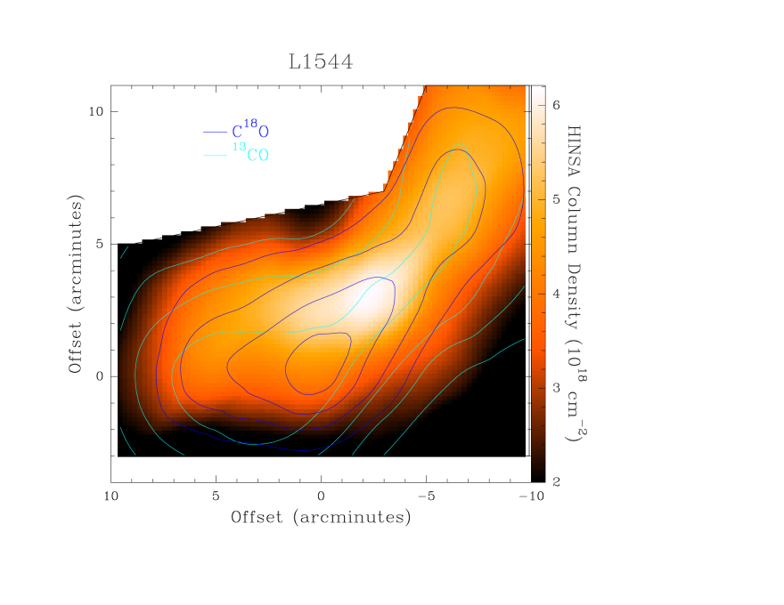
Figure 2: Maps of the cold HI column density producing narrow absorption features (HINSA in color; scale on right), contours of column densities of ¹³CO (blue), and of C¹⁸O (magenta) in L1544. The contours are at 30, 50, 70, and 90% of maximum values, which are $7.0\times 10^{15}$ cm^-2 for ¹³CO and $1.2\times 10^{15}$ cm^-2 for C¹⁸O.

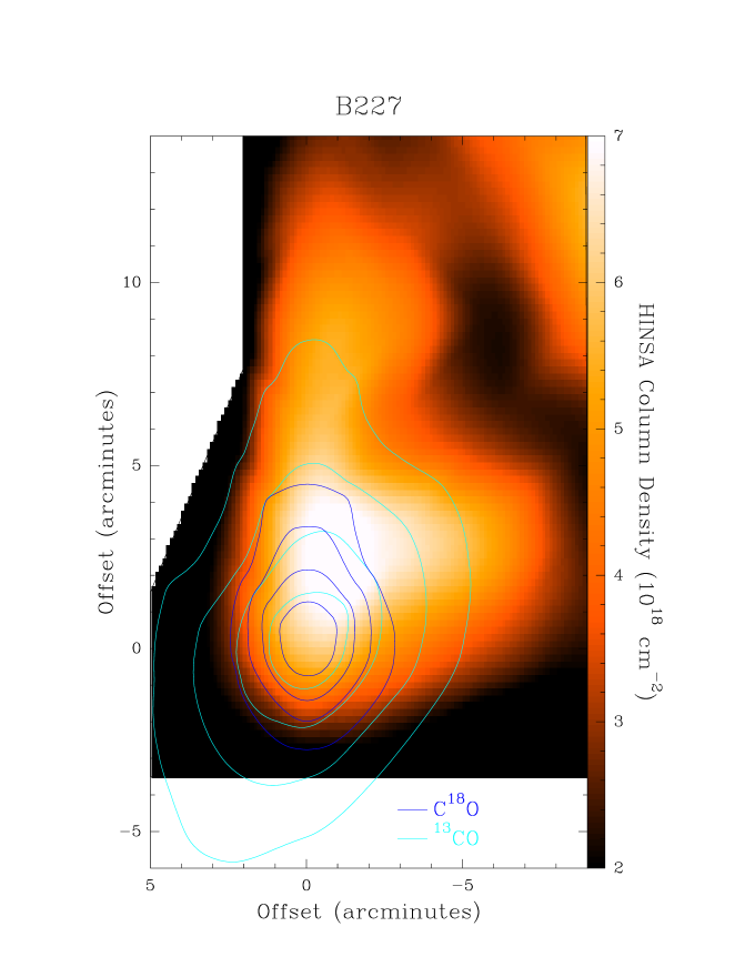
Figure 3: HINSA, ¹³CO and C¹⁸O column densities for B227. The color scale and relative contours are the same as in Figure 2. The maximum value of the column density is $3.1\times 10^{15}$ cm^-2 for ¹³CO and $0.26\times 10^{15}$ cm^-2 for C¹⁸O.

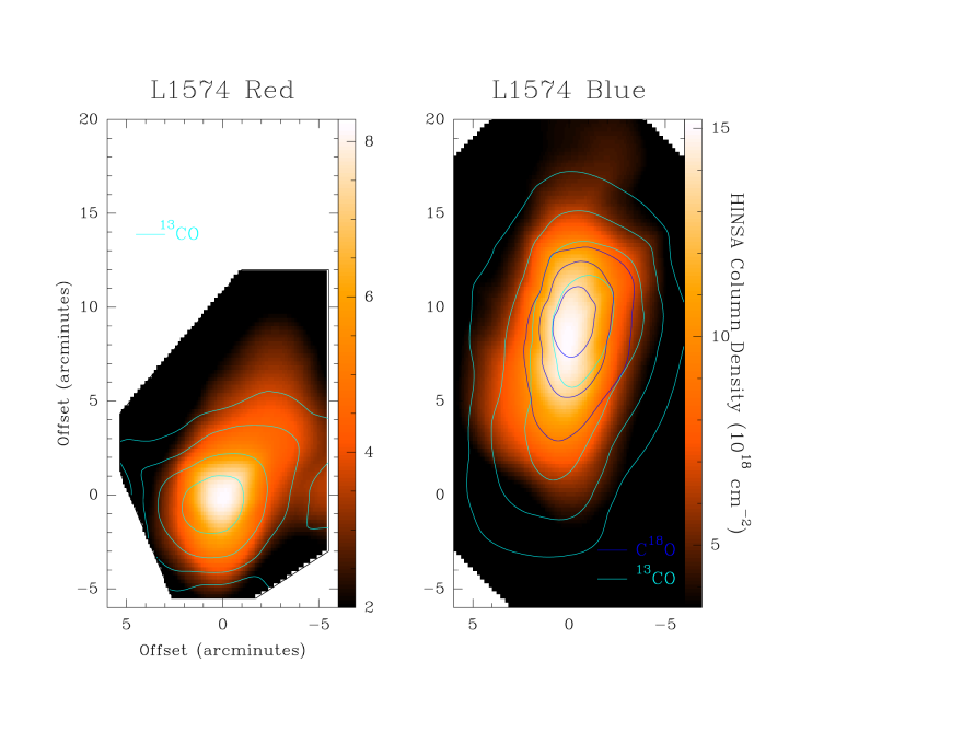
Figure 4: HINSA, ¹³CO and C¹⁸O column densities for L1574. The color scale and relative contours are the same as in Figure 2. For L1574b (velocity = 0 km s^-1), the maximum values of the column density are $3.6\times 10^{15}$ cm^-2 for ¹³CO and $0.51\times 10^{15}$ cm^-2 for C¹⁸O. For L1574r (velocity = 3.5 km s^-1), the maximum ¹³CO column density is $0.94\times 10^{15}$ cm^-2.

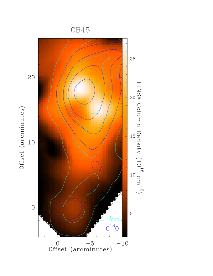
Figure 5: HINSA, ¹³CO and C¹⁸O column densities for CB45. The color scale and contours are the same as in Figure 2. The maximum values of the contours are $6.2\times 10^{15}$ cm^-2 for ¹³CO and $0.68\times 10^{15}$ cm^-2 for C¹⁸O.

3.7 CI

The only source sufficiently extended for its distribution to be probed by SWAS is L1544. In Figure 6 we show the integrated intensity of CI and the column densities of ¹³CO and cold HI (HINSA) along a cut in Right Ascension through the center of L1544. As indicated by the two–dimensional maps presented above, the ¹³CO and the cold HI basically track each other. The CI, however, shows a much less centrally–peaked distribution. Its intensity has dropped by a factor of less than two from the center to the edge of the map, while the ¹²CO and cold HI have diminished by a factor $\simeq$ 5. While the optical depth of CI may not be negligible, this data is strongly suggestive that the CI is predominantly in a relatively extended structure, and that the dense core with associated large column density seen in most molecular species does not dominate the CI emission from this dark cloud. This picture is supported by the relatively large line widths of the CI. As discussed in Li & Goldsmith (2003), these are generally much broader than those of HINSA or the carbon monoxide isotopologues. As shown in Figure 7 of that paper, the ¹³CO and HINSA line widths, which are largely nonthermal, are well correlated, while the CI line widths are essentially uncorrelated with those of HINSA and molecular species. In the case of L1544 our improved data here give a CI FWHM line width of typically 1.5 km s^-1. Comparison with the $\simeq$ 0.5 km s^-1 FWHM line widths of C¹⁸O and ¹³COindicates that the more extended region in which the CI is abundant has a larger turbulent velocity dispersion than does the region in which the molecular emission and HINSA absorption are produced.

Figure 6: Cut through the center of L1544 showing column density of ¹³CO (divided by a factor 1$\times 10^{15}$), the column density of cold HI producing the narrow HINSA feature (divided by a factor 1$\times 10^{18}$), and the integrated intensity of the CI ³P₁ – ³P₀ transition (multiplied by a factor of 4). The CI emission is clearly more spatially extended than the molecular emission or the HI absorption.

4 CORRELATIONS OF COLUMN DENSITIES

4.1 Carbon Monoxide Isotopologues

In order to trace as well as possible the molecular content of these clouds, we have compared the emission from ¹³CO and C¹⁸O. We see from Figure 7, where we plot N(¹³CO)/N(C¹⁸O) as a function of the C¹⁸O column density, that this ratio decreases systematically as N(C¹⁸O) increases, or as we move from the outer to the inner portions of the clouds. As mentioned above, the ¹³CO emission in the central part of L1544 suffers from moderate saturation, and we have corrected the optical depth and column density for this effect, as discussed above in Section 3.

Figure 7: Ratio of the ¹³CO to the C¹⁸O column density as a function of N(C¹⁸O). There is no data for the red component of L1574 as C¹⁸O has not been reliably measured in the 3.5 km s^-1 component of the cloud. The points for L1544 have been corrected for saturation as discussed in the text.

It is possible that the strong dependence of N(¹³CO)/N(C¹⁸O) on the column density of C¹⁸O is a result of uncorrected saturation in the more abundant species, but this seems unlikely for the following reasons. First, the L1544 data after correction for modest saturation (a factor $\leq$ 2 for the most saturated positions) agrees well with that of the other sources. Second, the line temperatures at the central positions having the strongest emission in the three other sources (Table 2), are significantly below the expected kinetic and J = 1$\rightarrow$0 excitation temperatures. Thus, saturation appears unlikely for the central positions of the three other sources, and very unlikely for the outer parts of these clouds. Third, the actual values of the ¹³CO to C¹⁸O ratio at the central positions of L1544, CB45, and L1574b (the peak of the blue velocity component at offset (0,9) relative to the cloud center) are all in the range 6 – 10, while the center of B227 has a ratio of 12.6. These values are basically consistent with the expected oxygen and carbon isotopic ratios (Langer & Penzias, 1990, 1993).

Our interpretation is that the ¹³CO to C¹⁸O ratio is being increased by isotope–selective processes operative in the outer parts of these dark clouds. Processes include chemical isotopic fractionation (e.g. Watson, Anicich, & Huntress, 1976) and isotope–selective photodissociation (e.g. Bally & Langer, 1982). The chemical isotopic fractionation is particularly effective in cold regions, but requires the presence of significant fraction of carbon in ionized form to operate. The isotope–selective photodissociation relies on reduced rates for this process resulting from self–shielding in line destruction channels. Studies including both processes indicate that chemical isotopic fractionation will be the dominant mechanism increasing the ¹³CO to ¹²CO ratio and the ¹³CO to C¹⁸O ratio at visual extinctions between 0.5 and 1 mag, if the gas temperature is $\simeq$ 15 K (Chu & Watson, 1983; van Dishoeck & Black, 1988). Both may work to increase the ¹³CO to C¹⁸O ratio and both become more effective in regions of reduced extinction where either the abundance of ionized carbon or the rate of photodestruction of carbon monoxide isotopologues is greater.

Plotting the ratio as a function of N(¹³CO) also shows a strong inverse correlation, similar to those of Langer et al. (1989) for a single cloud, B5. Those authors found a maximum of the ¹³CO to C¹⁸O ratio of approximately 30, close to the peak in Figure 7. We do not, however, find the drop in the column density ratio seen at the very outer edge of the cloud found by Langer et al. (1989). We feel that the results presented here suggest that ¹³CO is the superior probe of column density in the outer portions of these clouds. This is because the fractionation enhances the abundance of ¹³CO  and thus compensates for the overall drop in the molecular abundances in the outer portions of the cloud resulting from photodestruction. The good correlation of ¹³CO with visual extinction in the outer parts of clouds is further confirmation of this fortuitous cancellation of opposing effects.

4.2 OH

We have obtained OH emission spectra simultaneously with those of atomic hydrogen, and in Figure 8 we present a comparison between the OH column density and that of ¹³CO. For the sources other than L1544 there is no clear correlation, and while there is some segregation of the various clouds in terms of their total ¹³CO column density, there is no distinction to be made among them in the column density of OH. While a detailed explanation is beyond the scope of this paper, it does suggest that a large fraction of the OH emission resides in a “skin” of material in each cloud, and thus once a certain minimum column density (or visual extinction) is reached, the amount of OH present along the line of sight is essentially independent of the total column density. N(OH) shows a large scatter which may reflect the environment, the cloud density, or some combination of effects.

L1544 is the single cloud which the column densities of the two species are clearly correlated. The column densities are related as $<$N(OH)$>$ = 10${}^{-1.6}<$N(¹³CO)$>$ and N(OH) $\propto$ [N(¹³CO)]^0.6-0.7. The difference in behavior between this cloud the others observed may be related to its higher density and/or the more evolved state of this source.

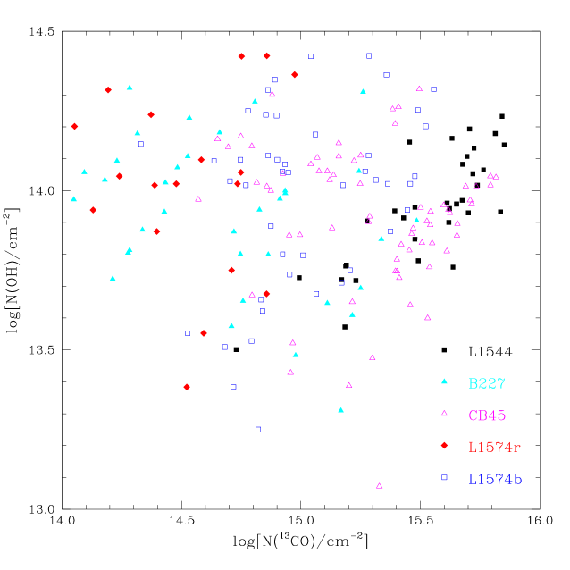
Figure 8: Column density of OH plotted as a function of the column density of ¹³CO. The ¹³CO data for L1544 have been corrected for saturation as discussed in the text.

4.3 Carbon Monoxide and Cold HI

In Figure 9 we show the correlation of the column densities of ¹³CO and cold HI in the four sources included in this study.

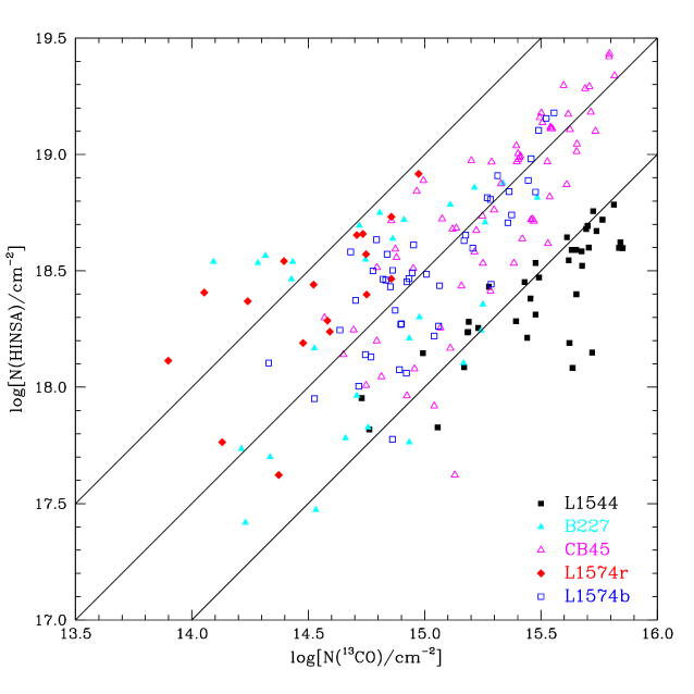
Figure 9: Plot of the column density of cold HI (HINSA) versus that of ¹³CO. The ¹³CO data for L1544 have been corrected for saturation. The three diagonal lines are not fits but represent ratios N(HINSA)/N(¹³CO) = 10^4.0 (highest), 10^3.5, and 10^3.0 (lowest).

Although there are some outlying points, it is clear that the column density of cold HI is highly correlated with that of ¹³CO. It is also clear that there is some difference in the ratio of the two column densities from one cloud to another. L1544 has the lowest ratio, $\simeq$ 650, B227, CB45, and L1574b are fit quite well by a ratio of 3100, and L1574r, by a ratio of 6300. Converting the ¹³CO column densities to total molecular column densities is complicated by the varying extinction that probably characterizes these different lines of sight. For reference, if we take a characteristic ratio N(¹³CO)/N(H₂) =  1.4$\times 10^{-6}$ (the value for Taurus from Frerking, Langer, & Wilson, 1982, omitting the offset term), the highest line in Figure 9 correponds to a ratio N(HI)/N(H₂) = 0.014, and the lowest line to a ratio a factor of 10 smaller.

Thus, while there is approximately a factor of 10 difference in N(HINSA)/N(¹³CO) between the cloud with the smallest and that with the largest value of this ratio, there is a clear correlation within each cloud which covers a range of $\simeq$ 20 in the column density of either species, and for the ensemble of clouds, covering a range of 100 in column density.

The values for the fractional abundance of HI that we have obtained are close to but somewhat larger than expected in a steady–state, and the implications of this are discussed in Section 7.

5 ATOMIC AND MOLECULAR DENSITIES

In order to extract the maximum value from the data about atomic hydrogen in molecular clouds, it is helpful to determine the actual number densities of different species. To do this, we model the density of HI, C¹⁸O, and ¹³CO in each cloud as a triaxial Gaussian, characterized by a peak value and three widths. We determine the two widths on the plane of the sky from the extent of the emission between half power points along two perpendicular axes. These are taken along (albeit imperfect) axes of symmetry for L1544, and along the directions of Right Ascension and Declination for the other three clouds.

The use of a Gaussian is reasonable given the column density distributions and the moderate dynamic range of our data. Given the $\simeq$ 3^′ angular resolution, we do not see any strong central peaking characteristic of the power law distributions often found for cloud cores; the small, dense regions are presumably significantly beam diluted in the present study. A Gaussian function makes it relatively easy to model the significant asymmetry seen to be characteristic of our sources, which is difficult to do with a power law density distribution. Using the distances given in Table 1, we obtain the FWHM source dimensions given in Table 4. The FWHM along the line of sight is taken to be the geometric mean of the two measured dimensions. The central density of species X is then given by

$$n_{cen}(X)=\frac{0.94N_{cen}(X)}{\Delta z_{FWHM~{}LOS}(X)}\>\>.$$ (1)

The HINSA and ¹³CO sizes for L1544 are lower limits due to incomplete coverage of the emission. This cloud is immersed in a region of lower column density (Snell, 1981) which extends to the northwest. The more extended maps suggest that the half power dimensions in this direction are only slightly greater than our limits. We see that the cloud dimensions in HINSA and ¹³CO emission are comparable, which suggests that these two species are coextensive. This is consistent with the fact that the ¹³CO nonthermal line widths are relatively close to those of HINSA (Li & Goldsmith, 2003).

The regions of C¹⁸O emission are smaller than those of HINSA or ¹³CO, but by a factor less than two. The C¹⁸O line widths are correspondingly smaller than those of HINSA. Thus, while the two molecular tracers both delimit regions comparable in size to that of the cold HI, it appears that the ¹³CO is probably the better tracer for comparison with the atomic hydrogen to determine fractional abundances. The central densities given in column 5 of Table 4 are intended to be representative of the central portion of the cloud, but given the moderate angular resolution of our observations and the fairly gradual fall–off of the densities, it is characteristic of a significant fraction of the cloud volume.

In order to determine the H₂ densities in the centers of the cloud, we have to adopt fractional abundances for C¹⁸O and ¹³CO; these inevitably are somewhat uncertain. In particular, depletion of carbon monoxide isotopologues onto dust grains, while not so evident as for some other species, is a potential problem for the densest, most quiescent regions of dark cloud cores (e.g. Caselli et al., 1999; Bacmann et al., 2002; Bergin et al., 2002; Tafalla et al., 2002; Redman et al., 2002). However, all of these studies indicate that significant depletion of rare isotopologues of carbon monoxide is restricted to the central, densest regions of clouds.

The map of CCS emission in L1544 (Ohashi et al., 1999) shows an elliptically shaped region approximately 1^′.5 by 3^′ in extent. There is evidently a central region in which is molecule is significantly depleted, but it is between 1^′ and 1^′.5 in diameter. A similar–sized region is heavily depleted in L1498 (Willacy, Langer, & Velusamy, 1998). For more distant clouds, regions of similar physical size (1.3 – 3 $\times$10¹⁷ cm) would appear smaller. These “depletion zones” are heavily beam diluted (by a factor $\simeq$ 10 in the single beam looking at the center of the cloud), and would of course be irrelevant for the vast majority of positions we have studied.

The region over which depletion has a major impact can also be seen in terms of the density required for significant depletion, which is $10^{5}$ – $10^{6}$ cm^-3 (Bacmann et al., 2002; Tafalla et al., 2002). This is basically two orders of magnitude greater than the average densities we find, consistent with the depletion being confined to a small portion of the line of sight as well as of the 3^′.3 beam. Using empirically determined density profiles, Tafalla et al. (2002) find that characteristic radii within which this density is attained are $\simeq$ 10¹⁷ cm, or 1^′.

The depletion rate is the rate of collisions which result on sticking to a grain. For molecules, the sticking coefficient $S$ is taken to be unity (Burke & Hollenbach, 1983), while for HI (see Section 6.1 below), $S$ = 0.3. The depletion rate is proportional to the sticking coefficient and inversely proportional to the square root of the particle’s mass (e.g. Draine, 1985). The depletion time scale is the inverse of this rate, which gives

$$\frac{\tau_{CO~{}depletion}}{\tau_{HI~{}depletion}}=1.6\>\>.$$ (2)

Scaling the results of Section 6.1 for molecular hydrogen formation to atomic hydrogen depletion and then to carbon monoxide depletion, we obtain $\tau_{CO~{}depletion}$ = 2.1$\times 10^{9}$/n${}_{H_{2}}$ yr. This is consistent with the results of Caselli et al. (1999) and Bacmann et al. (2002), that $\tau_{CO~{}depletion}$ $\simeq$ 10⁴ yr for n${}_{H_{2}}$ = 10⁵ cm^-3. The relatively short time scale for molecular depletion is thus a result of the very high densities in the cloud cores which overall have shorter evolutionary time scales than those characteristic of the lower density clouds in which they are embedded.

The modest effect of the depletion on determining the column density even in the beam including the cloud core is illustrated by the result of Caselli et al. (1999) who derive that the “missing mass” of H₂ from depletion of tracers is 2.3 solar masses in L1544. The column density in the central 3^′.3 beam assuming undepleted abundance of C¹⁸O is 4 solar masses. Thus, we could be underestimating the H₂ column density by as much as 50% in this direction. This would have the effect of decreasing the HI to H₂ abundance ratio in this (and possibly other) core directions, but would not change to an appreciable degree the correlation of HI and H₂ or the implications of the ratios determined.

Using the molecular hydrogen column densities and the source sizes, we derive the central densities of atomic and molecular hydrogen given in Table 5. We see that the atomic hydrogen densities are between 2 and 6 cm^-3. The density of molecular hydrogen derived from C¹⁸O is on the average a factor 1.7 larger than that derived from ¹³CO. As discussed above, the ¹³CO is probably a better tracer of the large–scale distribution of gas, but is more likely to miss material in the central region of the cloud due to uncorrected saturation. The results from both tracers are in reasonable agreement and we should have results from both in mind for comparison of the fraction of atomic gas measured here with that predicted from models presented in the following section.

6 TIME–DEPENDENT MODELING OF THE ATOMIC TO MOLECULAR HYDROGEN RATIO

6.1 Rate Equation for H₂ Formation

In order to calculate the gas phase abundances of atomic and molecular hydrogen, we need to model the grain surface production H₂. For the present study, we assume that all dust grains are spherical particles, differing only in their size. This neglects the changes in grain density and structure that could be a consequence of processes which initially formed the dust grains, or modified them by accretion or coagulation. But since the effects of grain evolution, particularly on the surface properties of grains which are critical for H₂ formation and molecular depletion are so uncertain, this simplification seems a reasonable starting point.

The basic equation giving the formation rate of H₂ molecules on the surfaces of grains of a single type, e.g. grains having a specified cross section and number density (Hollenbach, Werner, & Salpeter, 1971), is

$$R_{H_{2}}=\frac{1}{2}S_{HI}\epsilon_{H_{2}}n_{HI}<v_{HI}>\sigma_{gr}n_{gr}~{}.$$ (3)

$R_{H_{2}}$ has units of cm^-3 s^-1, $S_{HI}$ is the probability of a hydrogen atom which hits a grain sticking to it, and $\epsilon_{H_{2}}$ is the probability of a hydrogen molecule being formed by recombination of two hydrogen atoms and then being desorbed from the grain. The atomic hydrogen density in the gas is $n_{HI}$ (cm^-3), the mean velocity of these atoms is $<v_{HI}>$ (cm s^-1), while the number density of grains having cross section $\sigma_{gr}$ (cm²) is $n_{gr}$ (cm^-3).

The sticking coefficient, estimated to be 0.3 by Hollenbach & Salpeter (1971), has been studied in a quantum mechanical treatment by Leitch–Devlin & Williams (1985). These last authors considered physisorption and chemisorption on plausible grain surfaces of graphite, silicate, and graphite covered with a monolayer of water. The values of $S_{HI}$ found range from 0.9 to very small values. Given the uncertainties in grain composition and binding mechanisms, it appears reasonable to adopt the value $S_{HI}$ = 0.3.

For grain surfaces with binding sites of a single type, there is an inherent competition between thermal desorption and H₂ formation. If the binding is very strong, atoms on the surface will not desorb, but they will not be mobile, so the H₂ formation rate will be low. On the other hand, if the binding is very weak, the mobility will be high, but so will be the rate of thermal desorption, and again, the rate of formation of H₂ will be reduced. This has led to the concern that the formation rate of molecular hydrogen will be large only over a very narrow range of grain temperature, a result which would certainly be problematic given the wide range of temperatures characterizing clouds in which significant fractions of molecular hydrogen are found.

Cazaux & Tielens (2002) circumvented this problem by postulating two types of binding sites on individual grains - physisorption sites with relatively weak binding, and chemisorption sites characterized by 10 to 100 times stronger binding. At the temperatures of dense molecular clouds, there will always be atoms in chemisorption sites, because the thermal desorption time scale far exceeds any other. Thus, any hydrogen atom hitting the grain and sticking will end up in a physisorption site, from which it can tunnel to a chemisorption site where it finds a partner. The barrier between the two types of sites is moderate (E/k = 200 K), so that the effective mobility is high. Cazaux & Tielens (2002) show that for grain temperatures between 6 K and 30 K, $\epsilon_{H_{2}}$ is unity, and drops gradually to 0.2 for a grain temperature of 100 K. We adopt here $\epsilon_{H_{2}}$ = 1.0.

The grain mass per unit volume implied by the single type of grain assumed in equation 3 is given by

$$n_{gr}m_{gr}=\frac{n_{gas}<m_{gas}>}{GDR}~{},$$ (4)

where $m_{gr}$ is the mass of a grain, $n_{gas}~{}(\simeq n_{H_{2}}+n_{HI}+n_{He})$ is the total volume density of gas particles, $<m_{gas}>$ is the average mass of a particle in the gas, and $GDR$ is the gas to dust ratio by mass. The average mass per gas particle is

$$<m_{gas}>=\frac{(2n_{H_{2}}+n_{HI}+4n_{He})m_{p}}{n_{gas}}~{},$$ (5)

where $m_{p}$ is the mass of the proton. With this, we can write

$$n_{gr}\sigma_{gr}=n_{gas}\sigma_{gr}\frac{<m_{gas}>}{m_{gr}GDR}~{}.$$ (6)

The mass of a grain can be written $m_{gr}=\rho_{gr}V_{gr}$, where $\rho_{gr}$ is the density of a grain and $V_{gr}$ is its volume. Since we have no clear evidence that the grain density varies systematically with grain size, we adopt a single value of the grain density (typically $\simeq$ 2 gm cm^-3) for grains of all sizes. Associating $\rho_{gr}$ with the other grain parameters assumed to be independent of grain size, we can rewrite the H₂ formation rate as

$$R_{H_{2}}=\frac{S_{HI}\epsilon_{H_{2}}<v_{HI}><m_{gas}>}{2\rho_{gr}~{}GDR}\frac{\sigma_{gr}}{V_{gr}}n_{gas}n_{HI}~{}.$$ (7)

For grains of a single size, the H₂ formation rate is proportional to the ratio of the grain cross section to its volume. We can write the H₂ formation rate as

$$R_{H_{2}}=k_{H_{2}}n_{gas}n_{HI}\>\>,$$ (8)

where all of the other factors in equation 7 have been subsumed into

$$k_{H_{2}}=\frac{S_{HI}\epsilon_{H_{2}}<v_{HI}><m_{gas}>}{2\rho_{gr}GDR}\frac{\sigma_{gr}}{V_{gr}}\>\>.$$ (9)

For a single “standard” grain species of radius $a_{s}$, $\sigma_{gr}/V_{gr}$ = $3/4a_{s}$.

In Appendix A, we evaluate the effect of a grain size distribution on the rate coefficient for H₂ formation. With the simplest assumptions that all grains have the same density, and that the sticking coefficient and formation efficiency are independent of grain size, the effect of a power law distribution of grain radii can be analyzed straightforwardly, and for the Mathis, Rumpl, & Nordsieck (1977; hereafter MRN) size distribution, we find the particularly simple result given by equation A12 that $k_{H_{2}}$ depends only on the maximum and minimum values of the grain size distribution.

Defining the total proton density in atomic and molecular hydrogen as

$$n_{0}=n_{HI}+2n_{H_{2}}\>\>,$$ (10)

and including a standard helium abundance of 0.098 relative to hydrogen in all forms, we can write

$$n_{gas}<m_{gas}>=(1+\frac{4n_{He}}{n_{0}})m_{p}n_{0}=1.39m_{p}n_{0}\>\>,$$ (11)

which gives

$$R_{H_{2}}=k^{\prime}_{H_{2}~{}MRN}n_{HI}n_{0}\>\>,$$ (12)

with

$$k^{\prime}_{H_{2}~{}MRN}=\frac{S_{HI}\epsilon_{H_{2}}<v_{HI}>1.39m_{p}}{2\rho_{gr}GDR}\frac{3}{4a_{s}}\frac{a_{s}}{\sqrt{a_{max}a_{min}}}\>\>.$$ (13)

The final fraction represents the correction due to the grain size distribution, being equal to unity for any single grain size. Substituting standard values for the relevant parameters, and normalizing to them, we find

$$k^{\prime}_{H_{2}}=3.5\times 10^{-18}\frac{(\frac{S_{HI}}{0.3})(\frac{\epsilon_{H_{2}}}{1.0})({\frac{T}{10K}})^{0.5}}{(\frac{\rho_{gr}}{2gcm^{-3}})(\frac{GDR}{100})(\frac{a_{s}}{1.7\times 10^{-5}cm})}\frac{a_{s}}{\sqrt{a_{max}a_{min}}}~{}cm^{3}s^{-1}\>\>.$$ (14)

Based on the discussion in Appendix A, and the values for a Mathis, Rumpl, & Nordsieck (1977) grain size distribution with $a_{min}$ = 25 Å, $a_{max}$ = 10,000 Å, and $a_{s}$ = 1,700 Å, we find that the effect of the grain size distribution is to increase the formation rate coefficient by a factor of 3.4. We thus take a nominal value for $k^{\prime}_{H_{2}}$ = 1.2$\times 10^{-17}$ cm³s^-1.

The numerous factors which enter into the H₂ formation rate coefficient inevitably result in a relatively large uncertainty in this parameter. The range of values for the sticking coefficient $S_{HI}$ and the H₂ formation efficiency $\epsilon_{H_{2}}$ for “traditional” grains have been discussed earlier in this section. The grain density for grains of standard composition can vary by a factor $\simeq$ 1.5, and a similar variation in the gas to dust ratio is entirely plausible, although data in dark clouds is very sparse. The upper and lower limits on the grain size distribution enter as $(a_{max}a_{min})^{-0.5}$, but these quantities could easily differ from our adopted values by a factor $\simeq$ 2. It is also not clear whether very small grains would be effective for producing molecular hydrogen as their surface properties are likely very different from grains studied theoretically or measured in the laboratory. Combining the uncertainties in the various factors, $k^{\prime}_{H_{2}}$ may differ from its nominal value by a factor of 5. This directly impacts the H₂ formation time scale and the steady–state HI density, both of which vary as ${k^{\prime}_{H_{2}}}^{-1}$.

6.2 Time Dependence of HI and H₂ Densities

An idealized scenario for the evolution of the abundance of HI and H₂ consists of a cloud in which the hydrogen is initially entirely in atomic form, maintained in this state by photodestruction. At t = 0 the extinction is suddenly increased so that photodestruction in the bulk of the cloud volume (regions with visual extinction greater than $\simeq$ 0.5 mag) can be neglected. This is justified since the photodissociation rate of H₂ drops dramatically as a function of increasing column from the cloud surface, due to effective self–shielding (e.g. van Dishoeck & Black, 1988; Draine & Bertoldi, 1996).

To model the evolution of this cloud, we assume that the only destruction pathway for molecular hydrogen is cosmic ray ionization , which is assumed to occur at a rate $\zeta_{H_{2}}$ s^-1. The value of $\zeta_{H_{2}}$ in dense clouds has been found to lie in the range $10^{-18}$ to $10^{-16}$ s^-1 (Caselli, Walmsley, Terzieva, & Herbst, 1998), but in other studies has been more narrowly defined to be equal to $5\times 10^{-17}$ s^-1 (Bergin et al., 1999), and $(5.2\pm 3.6)\times 10^{-17}$ s^-1 (van der Tak & van Diskhoeck, 2000). This is consistent with results of Doty et al. (2002) from detailed modeling of the source AFGL2591.

A much higher ionization rate, $\zeta_{H_{2}}$ = $1.2\times 10^{-15}$ s^-1 found in diffuse clouds (McCall et al., 2003), can possibly be reconciled with the above if there is a component of the cosmic ray spectrum which penetrates diffuse but not dense clouds. Doty, Schöier, & van Dishoeck (2004) suggest that the much higher rate which they derive for IRAS 16293-2422 is actually being dominated by X–ray ionization from the central star, and that the true cosmic ray ionization rate is much lower. We here adopt the average of the values obtained by van der Tak & van Dishoeck, $\zeta_{H_{2}}$ = 5.2$\times 10^{-17}$ s^-1.

We assume that the evolution of the cloud takes place at a constant density, and write the equation expressing the time dependence of the molecular hydrogen (denoting the formation rate coefficient simply by $k^{\prime}$) as

$$\frac{dn_{H_{2}}}{dt}=k^{\prime}n_{HI}n_{0}-\zeta_{H_{2}}n_{H_{2}}\>\>.$$ (15)

Defining the fractional abundance $x_{i}$ (of atomic and molecular hydrogen) as the density of species $i$ divided by the total proton density, we find that

$$\frac{dx_{2}}{dt}=k^{\prime}x_{1}n_{0}-\zeta_{H_{2}}x_{2}\>\>.$$ (16)

Substituting equation 10 we can rewrite this as

$$\frac{dx_{2}}{dt}=k^{\prime}n_{0}-(2k^{\prime}n_{0}+\zeta_{H_{2}})x_{2}\>\>.$$ (17)

The solution is the time dependence of the fractional abundance of molecular hydrogen, given by

$$x_{2}(t)=\frac{k^{\prime}n_{0}}{2k^{\prime}n_{0}+\zeta_{H_{2}}}[1-exp(-t/\tau_{HI\rightarrow H_{2}})]\>\>.$$ (18)

The fractional abundance of atomic hydrogen is 1 – 2$x_{2}$, and hence is given by

$$x_{1}(t)=1-\frac{2k^{\prime}n_{0}}{2k^{\prime}n_{0}+\zeta_{H_{2}}}[1-exp(-t/\tau_{HI\rightarrow H_{2}})]\>\>.$$ (19)

The time constant for HI to H₂ conversion is given by

$$\tau_{HI\rightarrow H_{2}}=\frac{1}{2k^{\prime}n_{0}+\zeta_{H_{2}}}\>\>.$$ (20)

The steady–state molecular and atomic gas fractions can be found from equations 18 and 19, but in the limit of present interest $k^{\prime}n_{0}$ $\gg$ $\zeta_{H_{2}}$ we obtain

$$\tau_{HI\rightarrow H_{2}}=\frac{1}{2k^{\prime}n_{0}}\>\>.$$ (21)

The steady–state values for the constituents of the gas are then

$$x_{2}\rightarrow\frac{1}{2}~{}{\rm or}~{}n_{H_{2}}\rightarrow\frac{n_{0}}{2}\>\>,$$ (22)

and

$$x_{1}\rightarrow\frac{\zeta_{H_{2}}}{2k^{\prime}n_{0}}~{}{\rm or}~{}n_{HI}\rightarrow\frac{\zeta_{H_{2}}}{2k^{\prime}}\>\>.$$ (23)

This limit thus corresponds to our having essentially molecular gas, but the implication of equation 23 is that there is a constant density of atomic gas given by

$$n_{HI}(t\gg\tau_{HI\rightarrow H_{2}})\equiv n_{HI}^{*}=\frac{\zeta_{H_{2}}}{2k^{\prime}}~{}.$$ (24)

In Figure 10 we show the evolution of the atomic hydrogen fractional abundance as a function of time, for clouds in which the total proton density is fixed. From the discussion in Section 6.1 and Appendix A, we have adopted $k^{\prime}$ = $1.2\times 10^{-17}$ cm³s^-1 and $\zeta_{H_{2}}$ = $5.2\times 10^{-17}$ s^-1. This yields an equilibrium atomic hydrogen density $n_{HI}^{*}$ equal to 2.2 cm^-3. Equation 24 is not at all new; it was given by Solomon & Werner (1971), but their use of a much higher value of $\zeta_{H_{2}}$ resulted in an estimate of the equilibrium abundance of atomic hydrogen equal to 50 cm^-3, a value clearly ruled out by our data.

Figure 10: Time dependence of the fractional abundance of atomic hydrogen for clouds of fixed total proton density (in cm^-3). The curves of different total proton densities are logarithmically spaced at intervals of 0.25. The results for five sources studied here, located in terms of the atomic hydrogen to total proton density ratio and total proton density, are also included. The four sources with satisfactory solutions are indicated by open circles. B227, for which the fractional HI abundance is very close to the steady state value, is indicated by an arrowed box at the youngest age reasonably consistent with the data.

7 DISCUSSION AND IMPLICATIONS FOR CLOUD EVOLUTION

7.1 Cloud Age Based on Time–Dependent HI Fraction

For the nominal values we have adopted, the simple form of $\tau_{HI\rightarrow H_{2}}$ given by equation 21 will apply for n₀ $\gg$ $n^{*}$ = 2.2 cm^-3. In this limit, which is certainly relevant for dense clouds, the time constant is

$$\tau_{HI\rightarrow H_{2}}=\frac{8.3\times 10^{16}}{n_{0}}\ s=\frac{2.6\times 10^{9}}{n_{0}}\ yr\>\>.$$ (25)

Assuming that the clouds we have studied are characterized by densities determined from the ¹³CO observations, n₀ = 2 to 6 $\times 10^{3}$ cm^-3, and $\tau_{HI\rightarrow H_{2}}$ = 0.5 to 1.3 $\times 10^{6}$ yr. Using the larger densities from C¹⁸O reduces this characteristic timescale by a factor $\simeq$ two . As seen in Figure 10, the fact that the clouds observed have HI fractional abundances relatively close to steady–state values immediately indicates that the time elapsed since initiation of HI to H₂ conversion must be several times greater than $\tau_{HI\rightarrow H_{2}}$ or at least a few million yr. This “age” applies to the bulk of the molecular cloud as traced in ¹³CO and HINSA . For four of the five clouds studied, we obtain a unique solution for the elapsed time. This quantity, which we denote $\tau_{cloud}$, is defined by the total proton density (twice the molecular hydrogen density obtained from the ¹³CO column density and source size), and the fractional abundance of atomic hydrogen. While keeping in mind the uncertainty of the “age” as determined here, for these four dark clouds, this quantity lies in the range $10^{6.5}$ yr $\leq$ $\tau_{cloud}$ $\leq$ $10^{7}$ yr. The fractional abundance of atomic hydrogen in B227 is almost exactly the steady state value, and choosing a minimum time when this quantity will have dropped to close to this value leads to $\tau_{cloud}$ $\geq$ $10^{7}$ yr.

These relatively great cloud ages would pose a problem if there were clear evidence that these clouds were dynamically evolving. To evaluate this possibility, we have used the gaussian density distribution and the parameters derived above. Using the results from Appendix B and the masses and line widths given in Table 6, we calculate the potential and kinetic energies, ignoring surface effects, the external medium, and any contribution of the magnetic field. The clear result is that these clouds are close to virial equilibrium, with the possible exception of L1544, for which the numbers are particularly uncertain due to the incompletely defined extent of the cloud, but which appears to have $-\mathcal{U}$ noticeably larger than $2\mathcal{T}$. While this does not define the evolutionary path these clouds have followed, it does suggest that it is entirely plausible that they have spent several million years evolving to their present state .

In fact, we feel that these values for cloud ages must, for a number of reasons, be considered as lower limits. First, it is unlikely that the evolution of these clouds proceeds at constant density. Typical models of interstellar cloud evolution indicate that the path followed starts with lower–density atomic clouds and proceeds to higher density. This is not a requirement, in that if, for example, a compressive event initiates the process by compressing the gas and increasing the visual extinction, the density could immediately be increased to something like its final value, but in fact, no atomic clouds with even the moderate densities given in Table 5 have been observed. If cloud evolution includes an increase in the density occurring simultaneously with the HI to H₂ conversion, then much of the evolution will have taken place at lower densities than those now observed, and the time scale will be correspondingly longer. However, if the clouds were much more turbulent in the past and the turbulence were on a scale that affected the velocities of hydrogen atoms colliding with grains (see footnote 7), then the lower collision rate and H₂ formation rate resulting from the lower density would be partially offset by the higher HI–grain velocities.

Second, we may consider what happens if the column density is not sufficient to make photodestruction of H₂ insignificant in the central regions of these clouds. To first order, we can consider photodestruction of H₂ simply as adding to the cosmic ray destruction rate in equation 15. While formally increasing the time constant (equation 20), for clouds of high density, $\tau_{HI\rightarrow H_{2}}$ is unaffected, as long as n₀ $\gg$ [$\zeta_{CR}$ + $\zeta_{PHOTO}]/2k^{\prime}$. The models of Draine & Bertoldi (1996) suggest that the H₂ photodestruction rate will be comparable to the cosmic ray destruction rate adopted here for a column density of H₂ $\simeq$ $10^{21}$ cm^-2. Thus, while there could be a modest contribution from photodissociation to the total H₂ destruction rate, it will not be enough to change the time constant. However, the photodestruction will increase the steady–state abundance of HI. The fact that the values we have measured are only modestly above those expected solely from cosmic ray destruction of H₂ indicates that the effect is modest. If photodestruction plays a significant role, our solutions become lower limits to $\tau_{cloud}$ since they would, in effect, be steady–state values.

Third, as discussed in Section 5, we may have underestimated the column densities of molecular hydrogen, and hence n₀, along the lines of sight to the cores of these clouds. This may result in our having modestly overestimated n_HI/n₀ in these directions. This would have the effect of making the clouds look “younger” than they actually are.

Fourth, we must consider the possibility that there is not a reservoir of chemisorbed hydrogen atoms on the grain as postulated by (Cazaux & Tielens, 2002, 2004). Then, if the gas phase HI density and thus the adsorption rate is sufficiently low, one can reach a situation in which $<$N_HI$>$, the average number of hydrogen atoms on the grain, is less than unity. A newly–adsorbed incident atom may not find another atom with which to combine, and the H₂ formation rate will be reduced. This issue has been discussed by Biham et al. (1998) and Katz et al. (1999), and is consistent with laboratory measurements (e.g. Vidali et al., 1998). There is some concern whether the laboratory measurements are really applicable to the surfaces of interstellar grains, so that it seems appropriate to be cautious about the relevance of the measurements. If this picture is correct, the rate of H₂ formation for small grains is also reduced since $<$N_HI$>$ will also be less than unity. These effects combine to reduce the overall H₂ formation rate, particularly at relatively late times in the cloud evolution, when n_HI $\leq$ 100 cm^-3.

Additional support for our deteriming the minimum age of dark molecular clouds comes from modeling of the thermal evolution of gas which is in the process of converting hydrogen from atomic to molecular form. Each hydrogen molecule formed releases a few eV of energy into the gas. The exact value is uncertain due to unknown distribution of the 4.5 eV molecular binding energy between grain heating, internal energy of the H₂ (which is radiated from the cloud), and kinetic energy of the H₂, which eventually is thermalized (Flower and Pineau des Forêts, 1990). Under steady state conditions and high densities as we have seen in Section 6.2, the density of atomic hydrogen is $\simeq$ few cm^-3. This density of HI results from the balance between formation of HI via cosmic ray destruction of H₂ and destruction of HI by formation of HI on grains. In this situation, the heating from H₂ formation can be considered as a part of the cosmic ray heating, as it is the latter which supplies the energy to break the molecular bonds.

Early in the evolution of a cloud from atomic to molecular form, if we assume that the beginning of the process is characterized by a sharp increase in density to something approximating its current value, then the heating rate from H₂ formation is much larger, by a factor n₀/n${}_{HI}^{*}$ $\simeq$ 10³ (Goldsmith & Langer, 1978). The conversion of atomic to molecular hydrogen thus results in a reheating of the cloud (which had been cooling after the initial compression), to a temperature $\simeq$ 100 K (Flower and Pineau des Forêts, 1990). This reheating phase lasts for a time approximately equal to the characteristic HI $\rightarrow$ H₂ conversion time (equation 20), which is plausibly on the order of a million years. The fact that we see dark clouds which have obviously cooled to temperatures an order of magnitude below that sustained by the initial formation of molecular hydrogen is a further indication that the initiation of the molecular cloud phase must have taken place a minimum of a few million years in the past.

7.2 Other Effects and Concerns

Although the time–dependent evolution of the HI fractional abundance in the scenario developed above seems plausible, there are a number of other processes which may affect the abundance of atomic hydrogen and thus confuse this picture. One such effect is turbulent diffusion, in which the enhanced ability of material to move over significant distances increases the effect of concentration gradients (Xie, Allen, & Langer, 1995). Turbulent diffusion has been applied by Willacy, Langer, & Allen (2002) to the case of atomic hydrogen in dark clouds. Their results suggest that a quite modest values of the turbulent diffusion constant, K $\leq$ $5\times 10^{21}$ cm³ s^-2 are sufficient to produce atomic hydrogen densities in the centers of clouds similar to what we measure. This is not surprising, in the sense that our values are equal to or modestly greater than those expected for steady–state conditions with no turbulent diffusion.

It appears that while these values of K may be physically plausible, they are significantly smaller than those required for this model to reproduced various other chemical abundances in dark clouds. It is also the case that the atomic hydrogen column densities predicted by this model are significantly in excess of those that we observe. Thus, it is premature to say that the present observations indicate, in any significant way, that turbulent diffusion plays a very significant role. The results of Willacy, Langer, & Allen (2002) for the density of HI in the center of the model cloud are for $5\times 10^{6}$ yr of evolution of the cloud, and it is plausible that the timescale we have derived above still is relevant for reducing the HI density in the centers of dark clouds to the low values we have obtained.

A related model suggests large–scale circulation of gas in the cloud (Chièze & Pineau des Forêts, 1989). In this model, parcels of gas are exchanged between the outer, relatively unshielded portions of the cloud, and the interior. These authors analyzed the effect on a number of molecular species, but did not consider HI. However, it is reasonable that the effect would be to increase the HI density inside the cloud, as is the case for other species which are typically abundant only in regions of small visual extinction. While suggestive, it is difficult to make any quantitative comparisons with this model as no results for atomic hydrogen are reported.

We should consider the correlation between cold HI and molecular column density presented earlier in Figure 9. It is evident that in the context of a steady–state for HI production and destruction, the HI column density is proportional to the line of sight extent of the cloud, since the number density of atomic hydrogen is a constant. In this sense it is very different than the column density of e.g. ¹³CO, which is the integral of the number density of that species along the line of sight. For the HI, the extent of the cloud is be defined by two factors. The first of these is the size of the region in which the HI number density is more or less constant. Evidently, the fractional abundance of the HI will increase dramatically in the portion of the cloud with low extinction, but outside of some radius, the number density will become insignificant. The second factor is basically observational: since the absorption coefficient for HI varies inversely as the temperature, atomic hydrogen in the outer layers of the cloud is much less detectable than that in the cold interior. This effect is significant as the outer layers of the cloud even with standard radiation field can be at temperatures $\simeq$ 100 K, an order of magnitude higher than those in the cloud center.

It is appropriate here to follow up on this issue of warm HI surrounding that which we feel is well–mixed with the molecular material. Models of basically static clouds embedded in a much warmer, diffuse interstellar medium and irradiated by an interstellar radiation field (ISRF) have envelopes (“onion skins”) of ionized hydrogen, and neutral hydrogen, and ionized carbon, and neutral carbon (e.g. Abgrall et al., 1992; Le Bourlot et al., 1993). The self–shielding of the H₂ results in its abundance rising when the visible optical depth $\tau_{v}$ reaches 10^-4, and becoming comparable to that of HI for $\tau_{v}$ = 10^-1. The temperature will be 30 K and 100 K, for enhancement factors of the radiation field relative to the standard ISRF of 1 and 10, respectively.

The HI halos seen in emission around molecular clouds (e.g. Wannier, Lichten, & Morris, 1983; Andersson, Roger, & Wannier, 1992) correspond to these warm cloud edges where the fractional abundance of H₂ is dropping significantly. However, as discussed earlier, the very narrow line widths and low minimum line intensities that we are dealing with here indicate that we are observing much cooler and also less turbulent gas. The smaller spatial extent of HINSA absorption compared to the CI emission as well as its narrower line width (Section 3.7) is additional strong evidence that the HINSA column density is not significantly affected by the warm neutral/ionized cloud halos .

The cold HI and molecular column densities, as indicated by Figure 9 (as well as by the maps of their distributions), are quite well correlated. Given the very different distributions expected from theoretical models, this appears somewhat surprising, but may reflect to some degree the basic geometry of the clouds. While there is clearly a significant density gradient, these regions have a basically convex geometry in three dimensions, so that lines of sight with large column density do encompass larger dimensions with sufficient material to provide a significant contribution to the column of cold HI. More complete models including the spatial and temporal evolution of atomic and molecular hydrogen, as well as other species, will be necessary to assess how accurately the atomic to molecular abundance ratio in the centers of these clouds can be used to determine their age.

7.3 Upper Limit on the Cosmic Ray Ionization Rate

We can utilize our measurement of the atomic hydrogen density to set a useful upper limit on the cosmic ray ionization rate in reasonably well–shielded dense clouds. From equation 24 we can write the cosmic ray ionization rate in terms of the steady state atomic hydrogen density and the H₂ formation rate as

$$\zeta_{H_{2}}=2k^{\prime}_{H_{2}}n_{HI}^{*}\>\>.$$ (26)

The HI density we have measured is an upper limit to the steady state density of atomic hydrogen, since processes such as turbulent diffusion, imperfect shielding against photodissociation, and time–dependent cloud evolution all work to increase the atomic hydrogen density. As discussed in Section 6.1, the uncertainties in k${}^{\prime}_{H_{2}}$ are substantial, but an upper limit to k${}^{\prime}_{H_{2}}$ equal to 6$\times 10^{-17}$ cm³ s^-1 is reasonable. If we interpret our observations as giving n_HI = 4 cm^-3 as the upper limit to n${}_{HI}^{*}$, we find that $\zeta_{H_{2}}\leq 5\times 10^{-16}$ s^-1.

Our data, in common with many other observations of dark clouds, constrain the cosmic ray flux through the heating provided to dark clouds. In regions with visual extinction greater than a few magitudes, cosmic rays are expected to be the dominant heating source for the interstellar gas. At densities $\leq$ 10⁴ cm^-3 gas–dust coupling has only a very minor effect on the gas temperature, which is determined by the balance between cosmic ray heating and molecular line cooling (Goldsmith, 2001). The latter varies as the gas temperature to the 2.4 power for n${}_{H_{2}}$ = 10³ cm^-3 and 2.7 power for n${}_{H_{2}}$ = 10⁴ cm^-3

The minimum gas temperature is obtained with no depletion of coolant species, and for n${}_{H_{2}}$ in the range 10³ to 10⁴ cm^-3, we find that $T_{gas}$ = $T_{0}g^{0.4}$, where $g$ is the scaling factor for the cosmic ray heating rate relative to a reference value 10^-27 n${}_{H_{2}}$ erg cm^-3 s^-1. $T_{0}$ is equal to 10 K for n${}_{H_{2}}$ = 10³ cm^-3 and 13 K for n${}_{H_{2}}$ = 10⁴ cm^-3.

For our adopted cosmic ray ionization rate $\zeta$(H₂) = 5.2$\times$10^-17 s^-1, and taking $\Delta$Q = 7 eV as the average energy transferred to the gas per cosmic ray ionization in a region of low fractional ionization (Cravens & Dalgano, 1978), we obtain a heating rate $\Gamma$ = 5.8$\times$10^-28n${}_{H_{2}}$ erg cm^-3 s^-1. This heating rate corresponds to g = 0.58, which yields gas temperatures $T_{gas}$ = 8.0 K for n${}_{H_{2}}$ = 10³ cm^-3 and 10.5 K for n${}_{H_{2}}$ = 10⁴ cm^-3. These are in good agreement with the temperatures of clouds, 8 K to 10 K determined in many studies using ¹²CO (e.g. Li & Goldsmith, 2003), and ammonia (Tafalla et al., 2002). These temperatures are also in excellent agreement with the low central temperatures inferred from modeling preprotostellar cores (Evans et al., 2001).

To be consistent with measured values of the kinetic temperature, we cannot have $g$ substantially greater than unity. Taking a reasonable upper limit to be g = 1 yields $\Gamma_{cr}$ $\leq$ 1$\times 10^{-27}$n${}_{H_{2}}$ erg cm^-3 s^-1, and gives gas temperatures $T_{gas}$ = 10 K for n${}_{H_{2}}$ = 10³ cm^-3 and 13 K for n${}_{H_{2}}$ = 10⁴ cm^-3. A cosmic ray heating rate significantly greater than this value thus seems unlikely to characterize the dense regions in dark clouds. The much higher values that are sometimes inferred (e.g. McCall et al., 2003; Liszt, 2003) may be the result of local conditions or of more diffuse compared to denser regions, since it is relatively more difficult to depress the heating rate than to enhance it. The low temperature of molecular clouds such as those observed here also suggests that the upper limit for the cosmic ray ionization rate derived above may well be overly generous and that the actual value of $\zeta_{H_{2}}$ does not significantly exceed 10^-16 s^-1.

8 SUMMARY

We have carried out a study of four dark interstellar clouds to define better the location of the cold atomic hydrogen relative to the molecular component within these regions. The HI is traced through observations of narrow self absorption features (HINSA), which are seen against the general Galactic background. The molecular clouds are traced by observations of OH (Arecibo) and ¹³CO and C¹⁸O obtained at FCRAO. For comparisons between atomic and molecular species, our results are limited to regions $\geq$ 3^′ in size, and thus refer to moderate–scale structure of these clouds. The most quiescent well–shielded central regions, in which molecular depletion may be significant, are heavily beam–diluted in this study and thus are unlikely to be affecting our conclusions.

The extent of the cold HI is close to, but somewhat smaller than that of the ¹³CO, and larger than the size of the C¹⁸O  emitting region. This is consistent with results previously obtained by Li & Goldsmith (2003), in which the nonthermal line widths of the species follow this same ordering. The column density of cold HI is moderately well correlated with that of ¹³CO, which is consistent with the general impressions of the maps of the different species, and which further indicates that the atomic hydrogen we are observing is not in outer envelopes of these clouds, but is predominantly in well-shielded cold regions, again consistent with the low temperatures for the HINSA–producing gas derived by Li & Goldsmith (2003).

The mapping of ¹³CO and C¹⁸O isotopologues reveals that the ratio of the column density of these species rises sharply at the edges of the clouds. This is unlikely to be a result of any radiative transfer effect, but rather suggests that the abundance ratio is enhanced in regions of low extinction. This effect is consistent with chemical isotopic fractionation, which has been predicted to be significant where the abundance of ionized carbon is significant, but the temperature is still quite low. The enhancement of the ¹³C in carbon monoxide offsets the drop in the abundance of this molecule in the outer regions of clouds due to photodestruction. The result is that the size of the region over which the abundance of ¹³CO relative to H₂ remains relatively uniform is increased, and we feel that this isotopologue is to be preferred as a tracer of the large–scale cloud structure, although saturation effects in regions of largest column density must be considered.

Using the HINSA and ¹³CO data, we model these clouds and obtain the central densities of atomic hydrogen and H₂. The central densities of H₂ are 800 to $\simeq$ 3000 cm^-3, and those of cold HI are between 2 and 6 cm^-3. The ratio of the atomic hydrogen to total proton densities ranges from 0.5 to 3 $\times 10^{-3}$. The values of n${}_{H_{2}}$ from C¹⁸O are a factor of two larger than those from ¹³CO, and the fractional abundances of HI a corresponding factor lower. These absolute and fractional HI abundances are close to, but somewhat larger than those expected for steady–state balance between HI production by cosmic ray ionization of H₂, and production of this molecule by grain surface recombination of HI. The effect of a power law grain size distribution on the formation rate of H₂ molecules has been evaluated, and for a MRN distribution with reasonable upper and lower limits, we find that that H₂ production rate is increased by a factor of 3.4 over that for standard grains of radius 1700 Å.

A number of processes including mass exchange and turbulent diffusion may be playing a role in determining the abundance of atomic hydrogen in dark clouds, but it is not certain whether their contribution is significant. We assume that these clouds have been evolving at constant density since the time that the atomic to molecular transition was initiated by some process which suddently increased the visual extinction and eliminating photodestruction of H₂. In this idealized picture, the HI to H₂ ratio drops monotonically with time, and the time constant for the conversion is given by $\tau_{HI\rightarrow H_{2}}=2.7\times 10^{9}/n_{0}$ yr, where n₀ is the total proton density. For the central densities of these sources, the time constants are $\simeq$ $10^{6}$ yr, and the ages of these clouds are 3 to 10 million years. The relatively low fractional abundance of atomic hydrogen makes it extremely unlikely that the time since the compressive event starting the atomic to molecular transition is significantly less than this, since photodestruction and the other processes mentioned above increase the HI abundance, and thereby require that the grain surface production of H₂ be quite close to completion. The conversion of atomic to molecular hydrogen sets a quite large lower limit to the time scale for the “molecularization” of dense clouds, and thus for the overall process of star formation.

Appendix A Effect of Grain Size Distribution on H₂ Formation Rate

In order to investigate the effect of a grain size distribution, we start from equation 3. For a grain size distribution, again assuming other quantities are independent of grain size, we use equation 9, but must take the appropriate grain cross section and grain volume averaged over the grain size distribution . We can write the formation rate coefficient for a grain size distribution as

$$k_{H_{2}}=\frac{S_{HI}\epsilon_{H_{2}}<v_{HI}><m_{gas}>}{2\rho_{gr}GDR}\frac{\Sigma_{gr}}{V_{gr}}\>\>.$$ (A1)

Assuming a distribution of spherical grains, and taking the relative number of grains having radius between $a$ and $a+da$ to be $n(a)da$, we have

$$\Sigma_{gr}=\int n(a)\sigma(a)da~{},$$ (A2)

and

$$V_{gr}=\int n(a)V(a)da~{}.$$ (A3)

We assume a power law grain size distribution having the form

$$n(a)=n(a_{min})(\frac{a}{a_{min}})^{-\alpha}~{},$$ (A4)

where $a_{min}$ is the minimum grain radius and $a_{max}$ is the maximum grain radius ($a_{min}\leq a\leq a_{max}$). The power law exponent, $\alpha$, is 3.5 in MRN model, but is here left as a free parameter. The total density of grains (cm^-3) is given by

$$n_{tot}=\int n(a)da=\int^{a_{max}}_{a_{min}}n(a_{min})(\frac{a}{a_{min}})^{-\alpha}da~{}.$$ (A5)

Evaluating equation A5, we find

$$n(a_{min})=\frac{1-\alpha}{R^{1-\alpha}-1}\frac{n_{tot}}{a_{min}}~{},$$ (A6)

where $R$ is the ratio of maximum to minimum grain radius:

$$R=\frac{a_{max}}{a_{min}}~{}.$$ (A7)

The ratio of the integrated grain cross section to integrated grain volume is

$$\frac{\Sigma_{gr}}{V_{gr}}=\frac{3}{4a_{min}}\left[\frac{4-\alpha}{3-\alpha}\right]\frac{R^{3-\alpha}-1}{R^{4-\alpha}-1}~{}.$$ (A8)

The effect of grain size distributions characterized by different values of $\alpha$ on $\Sigma_{gr}/V_{gr}$ is shown as a function of $R$ in Figure 11.

In the limit of no grain size distribution (R $\rightarrow$ 1) we recover the expected result for spherical grains of a single radius, $a_{s}$,

$$\left.\frac{\Sigma_{gr}}{V_{gr}}\right|_{a=a_{s}}=\frac{3}{4a_{s}}~{}.$$ (A9)

We can consider various values of $a_{max}$ and $a_{min}$ by treating $a_{min}$ and $R$ as free parameters, but it is helpful to normalize to the cross section to volume ratio for a single grain size, which gives us

$$\frac{\Sigma_{gr}}{V_{gr}}\left/\frac{3}{4a_{s}}\right.=\frac{a_{s}}{a_{min}}\left[\frac{4-\alpha}{3-\alpha}\right]\frac{R^{3-\alpha}-1}{R^{4-\alpha}-1}~{}.$$ (A10)

Equations A8 and A10 are general, but of particular relevance to suggested astronomical grain size distributions, these expressions are well–behaved for all values of $\alpha\geq 0$, including e.g. 3 and 4.

Figure 11: Effect of grain size distribution with $n(a)\propto a^{-\alpha}$ on the ratio of the integrated grain cross section to the integrated grain volume. The H₂ formation rate is directly proportional to this ratio. The vertical axis is normalized to the value of $\Sigma_{gr}/V_{gr}$ for grains of a single radius $a_{min}$.

For a fixed value of $a_{min}$, $\Sigma_{gr}/V_{gr}$ decreases as $R$ increases. For $R$ $\gg$ 1, the ratio varies as $R^{-1}$ for 0 $\leq$ $\alpha$ $\leq$ 2.5, and has a logarithmic dependence for $R$ = 3.0 and 4.0. The MRN grain size distribution is characterized by $\alpha$ = 3.5. In this case, we find that, for all $R$,

$$\left.\frac{\Sigma_{gr}}{V_{gr}}\left/\frac{3}{4a_{min}}\right.\right|_{\alpha=3.5}=R^{-0.5}~{}.$$ (A11)

This particularly simple result facilitates assessing the impact of this grain size distribution. The unnormalized ratio of the integrated grain cross section to integrated grain volume can be written

$$\left.\frac{\Sigma_{gr}}{V_{gr}}\right|_{\alpha=3.5}=\frac{3}{4}\frac{1}{\sqrt{a_{max}a_{min}}}~{},$$ (A12)

indicating that for this value of $\alpha$, the H₂ formation rate is inversely proportional to the geometric mean of the extremes of the grain size distribution.

In order to interpret the effect of the grain size distribution quantitatively, we need to consider specific values of the “standard” single grain size, $a_{s}$, along with the specifics of the GSD defined by $a_{min}$ and $R$, in addition to $\alpha$. Normalizing relative to the single–sized grains, we find

$$\left.\frac{\Sigma_{gr}}{V_{gr}}\left/\frac{3}{4a_{s}}\right.\right|_{\alpha=3.5}=\frac{a_{s}}{a_{min}}R^{-0.5}=\frac{a_{s}}{\sqrt{a_{max}a_{min}}}~{}.$$ (A13)

The ratio of integrated grain cross section to integrated grain volume relative to the ratio for grains of a single radius is thus determined by the ratio of that single grain radius to the geometric mean of the maximum and minimum grain radii. A smaller grain has a larger surface to volume ratio, so a grain size distribution including grains that are all smaller than the standard grain, will have $\Sigma_{gr}/V_{gr}$ larger than $3/4a_{s}$. It is more meaningful to compare grain size distributions with the constraint $a_{min}$ $\leq$ $a_{s}$ $\leq$ $a_{max}$, so that for $R\rightarrow 1$, $(\Sigma_{gr}/V_{gr})/(3/4a_{s})$ $\rightarrow a_{s}/a_{min}=1$. Note that as long as $a_{min}$ $\leq$ $a_{s}$ $\leq$ $a_{max}$, the normalized grain cross section per unit grain volume is independent of the reference grain size $a_{s}$.

There is a vast and ever–expanding literature on the subject of the range of grain sizes in interstellar clouds. These should be considered relative to the “standard” dust grain size, which is based on fitting behavior of the extinction in the visible region of the spectrum (Spitzer, 1978, ch 7). A representative value of $a_{s}$ is 1700 Å.

The more diverse dust grain population includes grains having radii as small as 10 Å  which are transiently heated to $\simeq$ 10³ K in reflection nebulae by absorption of a single photon (Sellgren, 1984). The infrared emission of small grains is also seen from the edges of molecular clouds exposed to fairly standard interstellar radiation field (Beichman et al., 1988). The need for small grains (radius 5–20 Å) to explain diffuse infrared emission in a number of galaxies in addition to the Milky Way was emphasized by Rowan–Robinson (1992). Specific spectral features seen in the infrared led to recognition that the population of small grains may include polycyclic aromatic hydrocarbon (PAH) molecules (e.g.  Leger & Puget, 1984; Omont, 1986; Ryter, Puget, & Pérault, 1987; Puget & Léger, 1989), although very small grains may well have a significant graphite component (Désert et al., 1986).

There has been increasing evidence that a larger–than–standard grain size component exists in dense regions of the interstellar medium. The earliest indications of “grain growth” in these regions came from visual/infrared photometry (Carrasco, Strom, & Strom, 1973) and the wavelength dependence of polarization (Carrasco, Strom, & Strom, 1973; Brown & Zuckerman, 1975; Serkowski, Mathewson, & Ford, 1975; Whittet & van Breda, 1978; Breger, Gehrz, & Hackwell, 1981). Large grains (radius $\simeq$ 5000 Å) have been invoked to reproduce the spectral properties of reflection nebulae (Pendleton, Tielens, & Werner, 1990) and 30 $\mu$m (3$\times$10⁵ Å) radius grains added to a dust model to explain the emission observed at millimeter wavelengths (Rowan–Robinson, 1992).

Grain growth has also been inferred from the dependence of the long–wavelength (millimeter and submillimeter) spectral index of the dust emissivity on the column density and volume density in molecular clouds (Woody et al., 1989; Walker, Adams, & Lada, 1990; Goldsmith, Bergin, & Lis, 1997; Visser et al., 1998). These observations indicate that the frequency dependence (characterized by power law exponent $\beta$) of the grain emissivity or optical depth in dense regions of molecular clouds has $\beta$ less than 2, the standard value characteristic of grains in the general interstellar medium (e.g. Kogut et al., 1996). The observations of Stepnik et al. (2003) suggest that grain coagulation in a dense filament in the Taurus complex has resulted in a deficiency of small grains together with an enhancement of the submillimeter wavelength emissivity. Grain coagulation is a very complex and imperfectly understood process (see Draine 1985 and references therein), but can result in fluffy and highly non–spherical grains (Wright, 1987). The MRN grain size distribution may be significantly modified in regions where dsut coagulation has taken place, with a resulting uncertain effect on the H₂ formation rate.

Evidence for grain growth is very strong in even denser regions, particularly protostellar disks, which suggests that this is, in fact, a continuous process throughout all phases of the dense interstellar medium. In choosing nominal values for the maximum and minum grain sizes for use in evaluating the H₂ formation rate in fairly standard clouds, there is certainly a large range of possible values, but the effect of the uncertainty is mitigated by the fact that in e.g. equation A13 the dependence is on the geometric mean of $a_{max}$ and $a_{min}$. We adopt nominal values for radii $a_{max}$ = 10,000 Å and $a_{min}$ = 25 Å, which together with the the standard grain radius $a_{s}$ = 1,700 Å result in the grain size distribution increasing the H₂ formation rate by a factor of 3.4. This modest but significant value suggests that a plausible grain size distribution does increase the H₂ formation rate, but only in extreme cases where the grain size distribution has been heavily skewed to either very large or very small grains, will the formation rate coefficient $k^{\prime}_{H_{2}}$ be drastically affected by the grain size distribution.

Appendix B Potential Energy of Cloud with Gaussian Density Distribution

If we take the density distribution for a spherically symmetric cloud to be given by

$$n(r)=n_{0}e^{-(r/r_{0})^{2}}\>\>,$$ (B1)

the mass contained within radius $r$ is given by

$$M(r)=\pi r_{0}^{3}[\sqrt{\pi}~{}erfc(\frac{r}{r_{0}})-2(\frac{r}{r_{0}})e^{-(\frac{r}{r_{0}})^{2}}]\>\>,$$ (B2)

where $erfc$ is the error function. The total mass of the cloud is then given by

$$M=\pi^{3/2}n_{0}<m_{gas}>r_{0}^{3}\>\>,$$ (B3)

where $<m_{gas}>$ is the average mass of a gas particle, defined in equation 5.

The potential energy is given by the integral

$$\mathcal{U}=-G\int_{0}^{\infty}\frac{M(r)dm(r)}{r}\>\>,$$ (B4)

where $dm(r)$ is the mass in a shell at radius $r$. The integral is well–defined, and gives us the result

$$\mathcal{U}=-\frac{1}{\sqrt{2\pi}}\frac{GM^{2}}{r_{0}}\>\>.$$ (B5)

A fraction 0.90 of the mass is contained within radius $r_{90}$ = $1.768r_{0}$, and expressed in terms of this parameter, $\mathcal{U}=-0.71GM^{2}/r_{90}$, very similar to that for a $r^{-1}$ density distribution.

Table 1: Source Parameters

Name	RA(2000)	Decl (2000)	Distance	Reference
			(pc)
L1544	05 04 18.1	25 11 08	140	Elias (1978)
B227	06 07 28.4	19 28 04	400	Bok & McCarthy (1974); Arquilla (1984)
				Tomita, Saito, & Ohtani (1979)
L1574	06 08 05.0	18 28 12	300	Kawamura et al. (1998)
CB45	06 08 45.9	17 53 15	300	Kawamura et al. (1998)

Table 2: Peak T_mb (K) at Reference Positions of Sources

Name	OH	13CO	C18O
L1544(0,0)	1.5	5.9	2.4
B227(0,0)	0.36	2.6	0.41
L1574(0,9)	0.46	2.3	0.44
CB45(-3,18)	0.44	3.4	0.79

Table 3: Column Densities at Reference Positions

Name	N(HINSA)	N(OH)	N(13CO)	N(C18O)	N(H2)	N(H2)
	1019 cm-2	1014 cm-2	1014 cm-2	1014 cm-2	1021 cm-2	1021 cm-2
L1544	.42	1.7	70.	12.	6.0	8.4
B227	.61	.80	31.	2.6	3.2	2.8
L1574r (0,0)	.83	2.3	9.4	$\cdots$	1.7	$\cdots$
L1574b (0,9)	1.5	2.1	36.	5.1	3.6	4.3
CB45 (-3,18)	2.7	1.0	62.	6.8	5.4	5.3

Table 4: Cloud Dimensions and Central Densities of Different Species

Name	Species	$\Delta\theta_{FWHM}$	$\Delta$z${}_{FWHM~{}LOS}$	ncen
		(′)	(1018 cm)	(cm-3)
L1544	HINSA	$>$11.5	$>$1.3	$<$3.0
L1544	13CO	$>$14.3	$>$1.8	$<$3.7$\times 10^{-3}$
L1544	C18O	string09.3	string1.2	string9.4$\times 10^{-4}$
B227	HINSA	string08.1	string2.9	string2.0
B227	13CO	string08.4	string3.0	string9.6$\times 10^{-4}$
B227	C18O	string05.2	string1.9	string1.3$\times 10^{-4}$
L1574r	HINSA	string07.4	string2.0	string3.9
L1574r	13CO	string07.7	string2.1	string4.2$\times 10^{-4}$
L1574b	HINSA	string08.8	string2.4	string5.9
L1574b	13CO	string11.2	string3.0	string1.1$\times 10^{-3}$
L1574b	C18O	string06.2	string1.7	string2.8$\times 10^{-4}$
CB45	HINSA	string15.6	string4.2	string6.0
CB45	13CO	string12.0	string3.0	string1.9$\times 10^{-3}$
CB45	C18O	string10.0	string2.7	string2.4$\times 10^{-4}$

Table 5: Central Atomic  and Molecular Hydrogen Densities

Name	nHI	n${}_{H_{2}}$ from 13CO	n${}_{H_{2}}$ from C18O	nHI/n0	nHI/n0
	(cm-3)	(cm-3)	(cm-3)	from 13CO	from C18O
L1544	$<$3.0	$<$3100	string6400	$4.8\times 10^{-4}$	$2.3\times 10^{-4}$
B227	string2.0	string1000	string1200	$1.1\times 10^{-3}$	$8.3\times 10^{-4}$
L1574r	string3.9	string0800	string $\cdots$	$2.4\times 10^{-3}$	$\cdots$
L1574b	string5.9	string1100	string2400	$2.7\times 10^{-3}$	$1.2\times 10^{-3}$
CB45	string6.0	string1700	string1900	$1.8\times 10^{-3}$	$1.6\times 10^{-3}$

Table 6: Cloud Masses and Energies

Name	$\Delta v_{FWHM}$	$\sigma_{0}$	M	$2\mathcal{T}$	$-\mathcal{U}$
	(km s-1)	($10^{4}$ cm s-1)	($10^{35}$ g)	($10^{45}$ erg)	($10^{45}$ erg)
L1544	0.64	4.6	4.8	1.5	5.7
B227	1.08	7.9	6.7	4.8	6.6
L1574r	1.42	10.4	1.9	2.3	0.76
L1574b	1.43	10.5	7.6	9.1	8.5
CB45	1.50	11.0	13.	17.	25.

References

- Abgrall et al. (1992) Abgrall, H., Le Bourlot, J., Pineau des Forêts, G., Roueff, E., Flower, D.R., & Heck, L. 1992, A&A, 253, 525
- Andersson, Roger, & Wannier (1992) Andersson, B.-G., Roger, R.S., & Wannier, P.G. 1992, A&A, 260, 355
- Arquilla (1984) Arquilla, R. 1984, PhD Dissertation, University of Massachusetts, Amherst
- Bacmann et al. (2002) Bacmann, A., Lefloch, B., Ceccarelli, C., Castets, A., Seinacker, J., & Loinard, L. 2002, A&A, 389, L6
- Bally & Langer (1982) Bally, J. & Langer, W.D. 1982, ApJ, 255, 143
- Barranco & Goodman (1998) Barranco, J.A. & Goodman, A.A. 1998, ApJ, 504, 207
- Batrla, Wilson, & Rahe (1981) Batrla, W., Wilson, T.L., & Rahe, J. 1981, A&A, 96, 202
- Beichman et al. (1988) Beichman, C.A., Wilson, R.W., Langer, W.D. & Goldsmith, P.F. 1988, ApJ, 332, L81
- Bergin et al. (1999) Bergin, E.A., Plume, R., Williams, J.P., & Myers, P.C. 1999, ApJ, 512, 724
- Bergin et al. (2002) Bergin, E.A., Alves, J., Huard, T., & Lada, C.J. 2002, ApJ, 570, L101
- Biham et al. (1998) Biham, O., Furman, I., Katz, N., Pironello, V., & Vidali, G. 1998, MNRAS, 296, 869
- Bok, Lawrence, & Menon (1955) Bok, B.J., Lawrence, R.S., & Menon, T.K. 1955, PASP, 67, 108
- Bok & McCarthy (1974) Bok, B.J., & Mc Carthy, C.C. 1974, AJ, 79, 42
- Bowers, Kerr, & Hawarden (1980) Bowers, P.F., Kerr, F.J., & Hawarden, T.G. 1980, ApJ, 241, 183
- Breger, Gehrz, & Hackwell (1981) Breger, M., Gehrz, R.D., & Hackwell, J.A. 1981, ApJ, 248, 963
- Brown & Zuckerman (1975) Brown, R.L. & Zuckerman, B. 1975, ApJ, 202, L125
- Burke & Hollenbach (1983) Burke, J.R., & Hollenbach, D.J. 1983, ApJ, 265, 223
- Carrasco, Strom, & Strom (1973) Carrasco, L., Strom, S.E., & Strom, K.M. 1973, ApJ, 182, 95
- Caselli, Hasegawa & Herbst (1998) Caselli, P., Hasegawa, T. I. & Herbst, E. 1998, ApJ, 495, 309
- Caselli, Walmsley, Terzieva, & Herbst (1998) Caselli, P., Walmsley, C.M., Terzieva, R., & Herbst, E. 1998, ApJ, 499, 234
- Caselli et al. (1999) Caselli, P., Walmsley, C.M., Tafalla, M., Dore, L., & Myers, P.C. 1999, ApJ, 523, L165
- Cazaux & Tielens (2002) Cazaux, S. & Tielens, A.G.G.M. 2002, ApJ, 575, L29
- Cazaux & Tielens (2004) Cazaux, S. & Tielens, A.G.G.M. 2004, ApJ, 604, 222
- Charnley (1998) Charnley, S. 1998, ApJ, L121
- Chièze & Pineau des Forêts (1989) Chièze, J.P. & Pineau des Forêts, G. 1989, A&A, 221, 89
- Chu & Watson (1983) Chu, Y.-H. & Watson, W.D. 1983, ApJ, 267, 151
- Clemens & Barvainis (1988) Clemens, D.P. & Barvainis, R. 1988, ApJS, 68, 257
- Cravens & Dalgano (1978) Cravens, T.E. & Dalgarno, A. 1978, ApJ, 219, 750
- Désert et al. (1986) Désert, F.X., Boulanger, F., Léger, A., Puget, J.L., & Sellgren, K. 1986, A&A, 159, 328
- Destombes et al. (1977) Destombes, J.L, Marliere, C., Baurdy, A., & Brillet, J. 1977, A&A, 60, 55
- Dewangan, Flower, & Alexander (1987) Dewangan, D.P., Flower, D.R., & Alexander, M.H. 1987, MNRAS, 226, 505
- Doty et al. (2002) Doty, S.D., van Dishoeck, E.F., van der Tak, F.F.S., & Boonman, A.M.S. 2002, A&A, 289, 446
- Doty, Schöier, & van Dishoeck (2004) Doty, S.D., Schöier, F.L., & van Dishoeck, E.F. 2004, A&A, 418, 1021
- Draine (1985) Draine, B.T. 1985, in Protostars and Planets II, D.C. Black & M.S. Matthews, eds. Tucson: Univ. of Arizona, 621
- Draine & Bertoldi (1996) Draine, B.T. & Bertoldi, F. 1996, ApJ, 468, 269
- Elias (1978) Elias, J.H. 1978, ApJ, 224, 857
- Evans et al. (2001) Evans, N.J.II, Rawlings, J.M.C., Shirley, Y.L., & Mundy, L.G. 2001, ApJ, 557, 193
- Feldt & Wendker (1993) Feldt, C. & Wendker, H.J. 1993, A&AS, 100, 287
- Flower and Pineau des Forêts (1990) Flower, D. & Pineau des Forêts, G. 1990, MNRAS, 247, 500
- Flynn et al. (2002) Flynn, E., Jackson, J.M., Simon, R., Shah, R.Y., Bania, T.M, & Wolfire, M. 2002, BAAS 34, 1282
- Frerking, Langer, & Wilson (1982) Frerking, M.A., Langer, W.D., & Wilson, R.W. 1982, ApJ, 262, 590
- Garzoli & Varsavsky (1966) Garzoli, S.L. & Varsavsky, C.M. 1966, ApJ, 145, 79
- Gibson, Taylor, Higgs, & Dewdney (2000) Gibson, S.J., Taylor, A.R., Higgs, L.A., & Dewdney, P.E. 2000, ApJ, 240, 851
- Goldsmith & Langer (1978) Goldsmith, P.F. & Langer, W.D. 1978, ApJ, 222, 881
- Goldsmith, Bergin, & Lis (1997) Goldsmith, P.F., Bergin, E.A., & Lis, D.C. 1997, ApJ, 491, 615
- Goldsmith (2001) Goldsmith, P.F. 2001, ApJ, 557, 736
- Goodman et al. (1998) Goodman, A.A., Barranco, J.A., Wilner, D.J., & Heyer, M.H. 1998, ApJ, 504, 223
- Green et al. (2001) Green, N.J.B., Toniazzo, T., Pilling, M.J., Ruffle, D.P., Bell, N., & Hartquist, T.W. 2001, A&A, 375, 1111
- Heiles (1969) Heiles, C.H. 1969, ApJ, 156, 493
- Heiles & Gordon (1975) Heiles, C. & Gordon, M.A. 1975, ApJ, 199, 361
- Hollenbach & Salpeter (1971) Hollenbach, D. & Salpeter, E.E. 1971, ApJ, 163, 155
- Hollenbach, Werner, & Salpeter (1971) Hollenbach, D.J., Werner, M.W., & Salpeter, E.E. 1971, ApJ, 163, 165
- Katz et al. (1999) Katz, N., Furman, I., Biham, O., Pirronello, V. & Vidali, G. 1999, ApJ, 522, 305
- Kavars et al. (2003) Kavars, D.W., Dickey, J.M., McClure-Griffiths, N.M., Gaensler, B.M., & Green, A.J. 2003, ApJ, 598, 1048
- Kawamura et al. (1998) Kawamura, A., Onishi, T., Yonekura, Y., Dobashi, K., Mizuno, A., Ogawa, H., & Fukui, Y. 1998, ApJS, 117, 387
- Knapp (1974) Knapp, G.F. 1974, AJ, 79, 527
- Kogut et al. (1996) Kogut, A., Banday, A.J., Bennett, C.L., Górski, K.M., Hinshaw, G., & Reach, W.T. 1996, ApJ, 460, 1
- Langer et al. (1989) Langer, W.D., Wilson, R.W., Goldsmith, P.F., & Beichman, C.A. 1989, ApJ, 337, 355
- Langer & Penzias (1990) Langer, W.D. & Penzias, A.A. 1990, ApJ, 257, 477
- Langer & Penzias (1993) Langer, W.D. & Penzias, A.A. 1993, ApJ, 408, 539
- Le Bourlot et al. (1993) Le Bourlot, J., Pineau des Forêts, G., Roueff, E., & Flower, D. 1993, A&A, 267, 233
- Leger & Puget (1984) Leger, A. & Puget, J. L. 1984, A&A, 137, L5
- Leitch–Devlin & Williams (1984) Leitch–Devlin, M.A. & Williams, D.A. 1984, MNRAS, 210, 577
- Leitch–Devlin & Williams (1985) Leitch–Devlin, M.A. & Williams, D.A. 1985, MNRAS, 213, 295
- Li & Goldsmith (2003) Li, D. & Goldsmith, P.F. 2003, ApJ, 585, 823
- Lipshtat et al. (2004) Lipshtat, A., Biham, O., & Herbst, E. 2004, MNRAS, 348, 1055
- Liszt (2003) Liszt, H. 2003, A&A, 398, 621
- Mathis, Rumpl, & Nordsieck (1977) Mathis, J.S., Rumpl, W., & Nordsieck, K.H. 1977, ApJ, 217, 425 (MRN)
- McCall et al. (2003) McCall, B.J., Huneycutt, A.J., Saykally, R.J., Geballe, T.R., Djuric, N., Dunn, G.H., Semaniak, J., Novotny, O., Al-Khalill, A., Ehlerding, A., Hellberg, F., Kalhori, S., Neau, A., Thomas, R., Österdahl, F., & Larsson, M. 2003, Nature, 422, 500
- McCutcheon, Shuter, & Booth (1978) McCutcheon, W.H., Shuter, W.L.H., & Booth, R.S. 1978, MNRAS, 185, 755
- Melnick et al. (2000) Melnick, G.J., Stauffer, J.R., Ashby, M.L.N., Bergin, E.A., Chin, G., Erickson, N.R., Goldsmith, P.F., Harwit, M., Howe, J.E., Kleiner, S.C., Koch, D.G., Neufeld, D.A., Patten, B.M., Plume, R., Schieder, R., Snell, R.L., Tolls, V., Wang, Z., Winnewisser, G., and Zhang, Y.F. 2000, ApJ, 539, 77
- Minn (1981) Minn, Y.K. 1981, A&A, 103, 269
- Montgomery, Bates, & Davies (1995) Montgomery, A.S., Bates, B., & Davies, R.D. 1995, MNRAS, 273, 449
- Myers et al. (1978) Myers, P.C., Ho, P.T.P., Schnepps, M.H., Chin, G., Pankonin, V., & Winnberg, A. 1978, ApJ, 220, 864
- Offer & van Dishoeck (1994) Offer, A.R. & Van Dishoeck, E.F. 1994, MNRAS, 257, 377
- Ohashi et al. (1999) Ohashi, N., Lee, S.W., Wilner, D.J., & Hayashi, M. 1999, ApJ, 518, L41
- Omont (1986) Omont, A. 1986, A&A, 164, 159
- Pendleton, Tielens, & Werner (1990) Pendleton, Y.J., Tielens, A.G.G.M., & Werner, M.W. 1990, ApJ, 349, 107
- Pirronello et al. (1999) Pirronello, V., Liu, C., Roser, J. E. & Vidali, G. 1999, A&A, 344, 681
- Puget & Léger (1989) Puget, J.L. & Léger, A. 1989, ARA&A, 27, 161
- Redman et al. (2002) Redman, R., Rawlings, J.M.C., Nutter, D.J., Ward-Thompson, D., & Williams, D.A. 2002, MNRAS, 337, L17
- Rowan–Robinson (1992) Rowan–Robinson, M. 1992, MNRAS, 258, 787
- Ryter, Puget, & Pérault (1987) Ryter, C., Puget, J.L., & Pérault, M. 1987, A&A, 186, 312
- Sellgren (1984) Sellgren, K. 1984, ApJ, 277, 623
- Serkowski, Mathewson, & Ford (1975) Serkowski, K., Mathewson, D.S., & Ford, V.L. 1975, ApJ, 196, 261
- Shuter, Dickman, & Klatt (1987) Shuter, W.L.H., Dickman, R.L., & Klatt, C. 1987, ApJ, 322, 103
- Snell (1981) Snell, R.L. 1981, ApJS, 45, 121
- Solomon & Werner (1971) Solomon, P.M. & Werner, M.W. 1971, ApJ, 165, 41
- Spitzer (1978) Spitzer, L. Jr. 1978, Physical Processes in the Interstellar Medium (New York: Wiley)
- Stepnik et al. (2003) Stepnik, B., Abergel, A., Bernard, J.-P., Boulanger, F., Cambrésy, L., Giard, M., Jones, A.P, Lagache, G., Lamarre, J.-M., Meny, C., Pajot, F., LePeintre, F., Ristorcelli, I., Serra, G., & Torre, J.-P. 2003 A&A, 398, 563
- Tafalla et al. (2002) Tafalla, M., Myers, P.C., Caselli, P., Walmsley, M., & Comito, C. 2002, ApJ, 569, 815