Fluctuation Properties and Polar Emission Mapping of Pulsar B0834+06 at Decameter Wavelengths

Abstract

Recent results regarding subpulse-drift in pulsar B0943+10 have led to the identification of a stable system of sub-beams circulating around the magnetic axis of the star. Here, we present single-pulse analysis of pulsar B0834+06 at 35 MHz, using observations from the Gauribidanur Radio Telescope. Certain signatures in the fluctuation spectra and correlations allow estimation of the circulation time and drift direction of the underlying emission pattern responsible for the observed modulation. We use the ‘cartographic transform’ mapping technique to study the properties of the polar emission pattern. These properties are compared with those for the other known case of B0943+10, and the implications are discussed.

1 Introduction

The realization that individual pulses from pulsars display considerable and often systematic fluctuations (Drake & Craft 1968; Sutton et al. 1970; Backer 1973) followed soon after the discovery of pulsars. Though amplitude modulations of pulse components were reported in pulsars with single or multiple components in their average profiles, more systematic phase modulations or “drifting subpulses”, occurring in conal single (Rankin 1986) pulsars, received a closer attention from observers and theorists.

Deshpande & Rankin (1999; hereafter DR99), Deshpande & Rankin (2001; hereafter Paper-I), Asgekar & Deshpande (2001; hereafter Paper-II) and Rankin, Suleymanova & Deshpande (2003; hereafter Paper-III) have reported detailed studies of drifting subpulses of B0943+10 at frequencies in the range 35–430 MHz. The studies led to the identification of a system of sub-beams circulating around the magnetic axis of B0943+10 that was responsible for the observed steady drift pattern (see DR99). The 35-MHz & 103/40 MHz results (paper-II & paper-III) show remarkable similarity with the higher frequency observations. Paper-I introduced a ‘cartographic transform’ (and its inverse) which relates the observed pulse sequence to a rotating frame around the magnetic axis in order to map the underlying pattern of emission. The implied configuration and the sub-beam circulation relate well with that envisioned by Ruderman & Sutherland (1975; hereafter R&S), wherein the circulation results from ExB drift. Whether we observe an amplitude or phase modulation will, in this picture, depends largely on the viewing geometry for a given pulsar. Although the subpulse modulation in B0943+10 shows remarkable and rare stability, one expects an underlying system of discrete sub-beams and their apparent circulation to exist in other pulsars too. However, the related details and their possible dependence on pulsar parameters are yet to be explored and understood. Further progress would, therefore, need the identification and detailed studies of the emission/subbeam patterns to be extended to a sizable sample of pulsars. Some of the recent investigations on B0834+06 (preliminary results reported in Asgekar & Deshpande 2000; Asgekar 2002), B0809+74 (van Leeuwen et al. 2003), and B0826-34 (Gupta et al. 2004) represent attempts in this direction.

Here, we report single-pulse analysis of the pulsar B0834+06 at 34.5 MHz based on a series of observations using the Gauribidanur telescope. This pulsar displays a double profile at frequencies ranging all the way from 35 MHz to 1 GHz. It displays strong, alternate-pulse intensity modulation without any significant drift at meter wavelengths (see, e.g. Taylor, Jura & Huguenin 1969; Slee & Mulhall 1970; Sutton et al. 1970, Backer 1973). It also exhibits frequent, short nulls (Ritchings 1976). Thus, B0834+06 offers us a useful context to examine whether the different apparent (single-pulse) modulations, particularly the amplitude and phase modulations, share the same underlying cause.

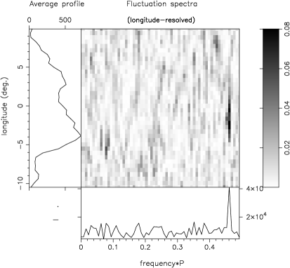
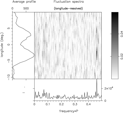
Figure 1: Longitude-resolved fluctuation spectra of sequences A & B. The strong primary fluctuation feature at 0.46 c/$P_{1}$ appears barely resolved for the B sequence (right panel). The corresponding A-sequence feature (left panel) is, on the other hand, relatively broad, indicating a quasi-periodic modulation.

Our observations and analysis procedures are outlined in the next section. The subsequent sections describe the results of fluctuation-spectral analysis and our basis for estimating the true frequencies of the modulation features in the spectra as well as the period and direction of the subbeam-system circulation. In the end, we present the derived polar emission maps and discuss our results along with their implications.

2 Observations and Analysis

Observations of B0834+06 were a part of a recent programme of pulsar observations (Asgekar & Deshpande 1999) initiated at the Gauribidanur Radio Observatory (Deshpande, Shevgaonkar & Sastry 1989) with a new data acquisition system for direct voltage-sampling (Deshpande et al. 2004). The pulsar was observed for a typical duration of $\mathrel{\hbox{\hbox to0.0pt{\hbox{\lower 4.0pt\hbox{$\sim$}}\hss}\hbox{$>$}}}{1000}$ s in each session. Several such observations were made during early 1999 and 2002. We discuss three data sets on B0834+06 below, denoted as ‘A’, ‘B’ and ‘C’, which were observed on February 5 & 6, 1999 and Feb. 5, 2002 respectively. Most of the analysis on sequence B consisted of 256 pulses, whereas that of sequence A & C consisted of 128 pulses, unless mentioned otherwise.

In paper-II we detailed our data acquisition system and reduction procedure used, and our techniques of spectral analysis are virtually identical to those used in Paper-I. Readers may refer to these papers for fuller descriptions of the above aspects.

3 Fluctuation Spectra

Longitude-resolved fluctuation (LRF) spectra (see Backer 1973) for the sequences A & B on B0834+06 are shown in Figure 1. Both spectra show a strong feature at $\sim 0.47$ c/$P_{1}$ (hereafter referred as feature-1), where $P_{1}$ denotes the rotation period of the pulsar. The feature appears barely resolved in the B-sequence spectrum, indicating a $Q$-value of $\sim 100$, found to be the highest among Qs seen in our pulse sequences. Sequence A, where the periodicity appears to be less stable, is more typical. This feature represents the alternate-pulse intensity modulation observed in this pulsar at meter wavelengths. The frequent, short nulls (typically 1 or 2 null pulses over $\sim 10-20$ pulses) may affect the $Q$-value of the modulation, as was noted by Lyne & Ashworth (1983) for pulsar B0809+74. However, due to inadequate sensitivity, we can not even assess, let alone quantify, the possible presence and effect of “nulls” in our data. The centroid frequency of feature-1 is slightly different for the two data sets, but such small variations ($\sim 1\%$) appear similar to those observed in B0943+10 (Paper-I, Paper-II & Paper-III).

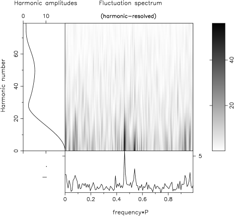
Figure 2: HRF-spectrum for sequence B data. A pair of features placed symmetrically around $0.5\,c/P_{1}$ are seen. Also seen are two sidebands on the primary fluctuation feature, which indicate the presence of a slower modulation in the data modulating the primary fluctuation (refer to text for details).

To examine the issue of possible aliasing of the spectral features here, we compute harmonic-resolved fluctuation spectra (hereafter, “HRF-spectra”, see paper-I: Figure 4) for the two pulse sequences A and B. An HRF-spectrum of a pulse sequence is computed by Fourier transforming the continuous time series, which is reconstructed from the (“gated”) pulse sequence by using the available samples on the pulse and filling the unsampled region with zeros. Such spectra can be computed for suitable blocks of 128 or 256 pulses and then the power spectra are averaged. We present, in Figure 2, the HRF-spectrum of the B sequence. The spectrum displays a pair of strong peaks at about 0.47 and 0.53 c/$P_{1}$. A similar spectrum for the A sequence (not shown) contains just these two features, but of about equal intensities. Such pairs of features in HRF-spectra represent the most general form of amplitude modulation (see, e.g. paper-I and Asgekar 2002); however an additional weak phase modulation cannot be ruled out. There is no clue as yet about the order of the aliasing of the primary modulation, although, as we will discuss later, the apparent modulation frequency is more likely to be 0.53 than 0.47 c/$P_{1}$.

In addition to the primary fluctuation features, in Figure 2 we also find another pair of features at $0.463\pm 0.069$ c/$P_{1}$ flanking the feature-1. Here, the side-tone product close to 0.4 c/$P_{1}$ is clearly seen (a frequency of $0.390\pm 0.001$ c/$P_{1}$), whereas the other (upper side-tone product) falls very close to the ‘alias’ component (at 0.53 c/$P_{1}$) of the primary fluctuation feature. These features suggest the presence of a slower, and most likely an amplitude, modulation on the primary fluctuation. The mean period of this slower modulation is estimated to be  $14.5\pm\,1.0\,P_{1}$, where the larger uncertainty reflects uncertainties in the estimation of frequency of the upper side-tone product located near 0.53 c/$P_{1}$. So, we observe a primary fluctuation which is modulated by a slower variation/fluctuation. Overall, this behavior is qualitatively similar to pulsar B0943+10. With this, we also note that there is an excess of power at $0.073\pm 0.007\,c/P_{1}$ (a period of $\sim 13.7\pm 1.4\,P_{1}$) in the LRF-spectrum computed from sequence B (see Figure 1b).

In most parts of sequence C, we find the same fluctuation spectral feature as seen in sequence A. However, in a small section of the C sequence, we notice an extreme situation where the alternate-pulse modulation feature (i.e. feature I) becomes very weak and the dominant modulation appears to be the slower one. This is clearly evident from the pulse sequence (Figure 3a), where strong emission is encountered about every 15 rotation periods. The fluctuation spectrum of this section of the data (Figure 3b) also reveals a strong feature at  0.06 c/$P_{1}$ that directly relates to the slow and deep modulation at a period of $15.0\pm\,0.8\,P_{1}$. Not surprisingly, this period is consistent with that suggested by the side-tones seen in the B sequence.

The three data sets presented here display almost a complete variety in the relative dominance of the two modulation features, and provide a remarkably consistent picture of their origin.

4 Aliasing, the circulation time, and drift direction

We now fold the pulse A & B sequences separately at their apparent primary fluctuation periods ($P_{3}$ tentatively identified as 1.856$P_{1}$ & 1.859$P_{1}$, respectively). The folded time series are displayed in Figure 4a,b.

The phase of the modulation (not shown) varies very slowly with pulse longitude and is not well defined at the centre of the profile. The intrinsic phase pattern is also likely to be smeared by a 5-bin smoothing we performed to improve the visibility of the otherwise weak pulses. The apparent average rate of this phase variation is small ($\leq 4\,^{\circ}\!/^{\circ}\!$), consistent with the primary feature being associated with an amplitude modulation.

The folded sequences also show that the modulation patterns under the two components of the average profile are possibly shifted in phase with respect to each other (Figures 4a,b), but only slightly. The exact delay is difficult to measure due to the very patchy nature of the intensity patterns. However, in our estimation the magnitude of the apparent relative delay between the modulations is within about 0.1 of the modulation cycle, or  0.2 $P_{1}$, corresponding to the longitude separation of the peaks of the two well-defined components in Figure 4b.

The relative delay in the modulation under the two components can be expressed, in general, as

$$\delta\zeta=(X+m)\,,with\,\,m=...-2,-1,0,1,2...;$$ (1)

where, $X$ is the apparent phase (or delay) difference between the modulations under the two components expressed as a fraction of the modulation period, and the integer $m$ accounts for the possible undetected integral cycles of the modulation phase as well as asserts the sense/direction of the drift (when combined with $X$). For the folded version of sequence A shown, $X$=0.1, and $X$=-0.1 if the data were to be folded at $P_{3}$=2.169 $P_{1}$. For the B sequence, we estimate $X$= -0.05 for the presently assumed $P_{3}$, and $X$ = 0.05 for the corresponding longer $P_{3}$ (Figure 4).

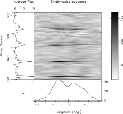
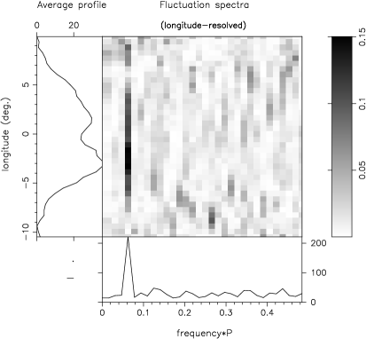
Figure 3: (Left) A 64-pulses long section of the C sequence shown in gray-scale; and (Right) longitude-resolved spectrum of this section of the sequence. Note the strong feature at 0.07 c/$P_{1}$ and the near absence of modulation feature at 0.46 c/$P_{1}$.

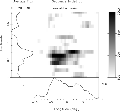
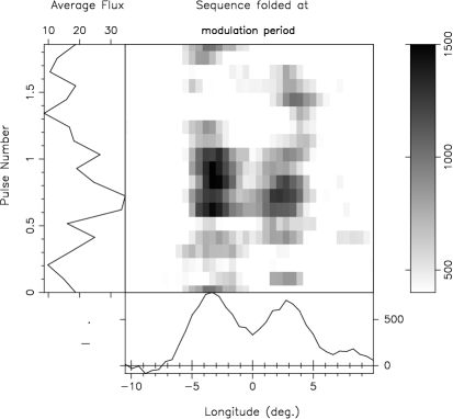
Figure 4: (Left) Sequence A folded at a modulation period of $P_{3}$ = 1.856 $P_{1}$. The relative delay in the modulation peaks under the two components is evident. A similar pattern would be seen even if the other possible $P_{3}$ (i.e. , 2.169$\,P_{1}$) were to be used for folding; then, any “drift” (or relative delay) would appear in the opposite sense. (Right) Sequence B folded at a $P_{3}$ of 1.859 $P_{1}$.

We interpret the relative delay between modulation under the two components as caused by the ‘passage’ of the same emission entity through our sightline as the polar-emission pattern rotates steadily around the magnetic axis. We can write the geometrical relationship between the rotational longitude $\delta\varphi$ and magnetic azimuth angle $\delta\theta$ as,

$$\delta\theta\,=\,sin^{-1}\left[sin(\alpha+\beta)sin(\delta\varphi)/\mid sin(r_{\varphi})\mid\right],$$ (2)

where $r_{\varphi}$, the associated magnetic latitude at the component longitudes, can be computed using the following well known relation

$$sin^{2}(r_{\varphi}/2)=\,sin^{2}(\delta\varphi/2)sin(\alpha+\beta)sin(\alpha)+sin^{2}(\beta/2)$$ (3)

A rotational longitude separation of the component peaks of  $\Delta\varphi=6.2^{\circ}\!$ (i.e. $\Delta\varphi=\pm 3.1^{\circ}\!$) implies a magnetic longitude separation $\Delta\theta\simeq 50^{\circ}\!$ (i.e. $\delta\theta\simeq\pm 25^{\circ}\!$) around the magnetic axis of the star. We can now directly estimate the circulation time of the pattern using eq. (2). Assuming that the polar cap periphery is roughly circular (see, for example, paper-I; Mitra & Deshpande 1999), the circulation time is given by

$$\hat{P}_{3}=\left(\frac{360^{\circ}\!}{\Delta\theta}\right){\delta\zeta}P_{3}$$ (4)

or, with eq. (1),

$$\hat{P}_{3}=\left(\frac{360^{\circ}\!}{\Delta\theta}\right)(X\,+m)\,P_{3}\;\,\,(m=\ldots,-1,0,1,2,\ldots),$$ (5)

where $\Delta\theta$ is the magnetic-longitude separation (in degrees) of the two component peaks.

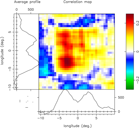
Figure 5: Longitude-longitude correlation of intensity fluctuations at a relative delay of 2 pulse periods, computed for B sequence data (of some 350 pulses). The intensity fluctuations at each longitude bin, shown along the horizontal axis, are cross-correlated separately with the fluctuations seen two pulse period later at every longitude bin indicated along the vertical axis. The central panel gives this correlation map according to the color scale at the right. The bottom and the left panels show the average profiles for the original B sequence and for the delayed version of it, respectively. The colour-scale used to display the correlation coefficients in the map is shown on the right. The observed correlation map is asymmetric w.r.t.  to the diagonal. The sense of the asymmetry indicates a subpulse “motion” from earlier to later longitudes.

If the observed amplitude modulation is generated by the steady rotation of a stable pattern around the magnetic axis, it should produce fluctuations having a period equal to the circulation time. The estimates for the two sequences and different values of $m$ are to be compared with our estimates of the circulation time as suggested by the slower modulation period (i.e.,  14.8 $P_{1}$ or so). It can be shown that the compatible values of $m$ are +1 and -1. Given the uncertainties in the various relevant parameters, it is not possible as yet to conclusively estimate the sign of $m$.

To help resolve this issue, we have chosen intensity sequences corresponding to two longitudes intervals symmetrically placed around the central (zero) longitude and with a separation of 6${}^{\circ}\!$ in order to examine their cross-correlation. In every one of the three sequences (i.e., A, B, & C), we find that the cross-correlation has a peak when the earlier longitude data is delayed by two pulse periods w.r.t. that at the later longitude, in clear contrast with the other way around. This clearly implies that $m$=+1, and that the drift direction is from earlier longitude to later— i.e., opposite to the pulsar rotation direction.

A further related confirmation of the drift direction (relative to the pulsar rotation) comes from longitude-longitude correlation maps of pulse sequences over delays of integer number of pulse periods (such an analysis was first used by Popov & Sieber 1990). The correlation map computed for sequence A is displayed in Figure 5, where the estimated (normalized) correlation between fluctuations in the intensity at a range of longitudes (marked along the horizontal axis) and the fluctuations observed two pulse-period later (at the various longitudes marked along the vertical axis) is shown.

Significant auto-correlation (i.e., along the +45${}^{\circ}\!$–slope line) is apparent at this delay of $+2\,P_{1}$, which is related to the primary modulation periodicity seen in this pulsar. The cross-correlation map, however, is not diagonally symmetric (about the +45${}^{\circ}\!$–slope line) for a delay of two rotation-periods, that is, the delayed versions of later-longitude sequences do not correlate with those at earlier longitudes. This we interpret as subpulse “motion” from earlier to later rotational longitudes, i.e. , positive drift.

Thus, we have identified an internally consistent configuration of the underlying circulating subbeam system responsible for the observed modulation. Based on various different signatures, we have indeed been able to estimate the circulation time, and find that $14.8\pm 0.8\,P_{1}$ is a value consistent with our observed sequences. It is worth pointing out that the actual circulation time is likely to be somewhat shorter than the above value (by typically 1 $P_{1}$), given the typical frequency of nulls. The drift direction is also determined above, and the sense of the PA sweep is known from the existing polarization data.

The alias ambiguity of the primary modulation feature, however, has yet to be resolved; but this is really only of academic interest, since our further investigations based upon emission mapping, etc, do not depend on its resolution. As we will mention later, it is possible to simply look at the average sequence over several circulation times and estimate the apparent spacing between successive sub-beams.

None of our derived estimates so far depend crucially on an accurate knowledge of the viewing geometry, although it was useful in determining the value of $m$, and the geometry will be an explicit ingredient in the cartographic transform to be used for emission mapping. We note that the available polarization measurements on this pulsar do not effectively constrain the viewing geometry, especially the sign of $\beta$.

5 Viewing Geometry of B0834+06

B0834+06, based on its double profile, is a member of the “D”-class according to the Rankin classification. The emission of this pulsar is believed to arise from the inner conal ring, and the geometrical parameters were derived accordingly (Rankin 1993).

The ‘inverse’ of the cartographic transform provides a powerful “closure” path to verify and refine the input parameters used to produce the polar map (see paper-I and Deshpande 2000, for a detailed discussion of this point). We wished to reconfirm the drift direction and “tune” our estimate of the circulation time. We also wanted to further constrain the assumed viewing geometry using this approach, if possible. To achieve this we carried out a grid search, where we varied the values of $\alpha$, $\beta$ and $\hat{P_{3}}$ over a reasonably wide range and alternated the drift direction as a parameter. For each different combination of the parameters in the search, we constructed an average-polar map from the observed sequence. The inverse transform was used to generate an artificial sequence from this trial polar emission pattern. We then cross-correlated (longitude by longitude) the artificial sequence with the natural (observed) one. The parameter combination for which the procedure yielded a higher cross-correlation coefficient, averaged over the longitudes, was considered a better indicator of the true values.

For B0834+06, the closure technique involving the inverse transform turns out to be rather insensitive to changes in the values of $\alpha$ and $\beta$ ($\alpha$ being larger for B0834+06 than for B0943+10) and the sign of $\beta$ was not constrained (see, Asgekar 2002). The technique was, however, sensitive to the circulation time and the drift direction, which allowed us to constrain these parameters. This, in a way, also meant that our resulting polar emission maps were rather insensitive to uncertainties in $\alpha$ and $\beta$. In what follows, we use the following set of refined parameters: $\hat{P_{3}}=14.84P_{1}$; $\alpha=30^{\circ}\!$; $\beta=-3^{\circ}\!.0$, with the drift direction same as that of the pulsar rotation. The resolution of the drift direction is then tied to the ambiguity in the sign of $\beta$, and a comparison with Ferraro’s theorem (Ruderman 1976) is possible after an unambiguous determination of $\beta$.

6 Polar Maps and Movies

We created the polar emission maps for the three pulse sequences discussed earlier using the cartographic transform mapping technique of Deshpande & Rankin (DR99, paper-I). Also, series of maps, each from successive short subsequences (of duration $\geq\,\hat{P}_{3}$) and with a large fractional overlap with the neighboring ones, were generated. The resulting images were viewed in a slow ‘movie’-like fashion. Since a polar map over one circulation time for B0834+06 doesn’t sample the entire polar cap adequately, each movie frame was made using 30 pulses (roughly twice the circulation time $\hat{P_{3}}$). We further smoothed this pattern over $10\times 10$ points in order to reduce the noise contribution, the smaller number of sub-beams making such smoothing practical. The movies allowed us to study variation of the polar emission pattern over the duration of the observation. Here, we present our maps and the insights gained by studying the movies.

6.1 Sequence-A ($5^{th}$February 1999)

The polar map for this sequence is shown in Figure 6a. Only a couple of distinct sub-beams are seen in the average polar map, whereas short averages corresponding to the frames of the movie show us more distinct sub-beams that fluctuate around their mean positions and in brightness. Patterns of strong, distinct sub-beams appear on the scales of $\sim 2\hat{P}_{3}$, giving rise to weak (Q-value $\mathrel{\hbox{\hbox to0.0pt{\hbox{\lower 4.0pt\hbox{$\sim$}}\hss}\hbox{$<$}}}100$) primary fluctuation features in the spectra. On the whole a few sub-beams dominate the maps over short intervals, similar to the case of sequence B below. Such ‘prominences’ last only about two circulation times, where after those sub-beams become weak and some others more prominent.

The bright sub-beams that dominate the emission in a movie frame appear to be broader than the average. Assessing the significance of this impression is difficult given both the smoothing and the noise present, but at times two adjacent bright sub-beams appear to touch each other.

The bright, isolated emission patches near the outer periphery of the region mapped are due to occasional extraordinarily bright single pulses in our sequence. We discuss these below.

6.2 Sequence-B ($6^{th}$ February 1999)

This sequence shows the sharpest primary fluctuation feature which has a $Q$-value $\sim 100$. Its polar map, presented in Figure 6b, shows a system of distinct sub-beams. Similar to the observations of B0943+10, the brightness of individual sub-beams appear to fluctuate with time. In fact, they vary by factors of almost 5 between certain short averages. At any given time a few sub-beams dominate the emission and overshadow emission from the rest of the polar cap. The individual subbeams here are generally less stable compared to those of B0943+10, and show an increased tendency to fluctuate around their mean positions —which may explain the lower Q value of this star’s primary fluctuation feature.

We would like to attract the reader’s attention to the part of the map where five roughly equi-spaced sub-beams span almost exactly half of the magnetic longitude range. It is clear from this configuration that the true $P_{3}$ is about 1/8^th of the circulation time, i.e. less than 2$\,P_{1}$. This, then, finally appears to resolve the aliasing issue. The LRF feature at 0.47 $c/P_{1}$ is indeed an alias of the true modulation frequency of $\sim 0.53$ $c/P_{1}$, making the unaliased $P_{3}$=1.859 $P_{1}$. This, in turn, implies the typical number of subbeams to be 8, a number also consistent with the estimates of magnetic azimuthal separation of the subbeams (as in section 4). Nonetheless, the subbeams spacing is not as uniform as in B0943+10.

6.3 Sequence-C ($5^{th}$February 2002)

The short 64-pulse sequence mapped here exhibits a deep periodic modulation that reflects the circulation cycle directly. Only a single dominating emission region is apparent. The streaky and highly elongated shape of the active region is the result of poor sampling and inadequate averaging across the map area. This extreme situation is rare as well as rewarding, in the sense that it permits us a direct estimation of the circulation period.

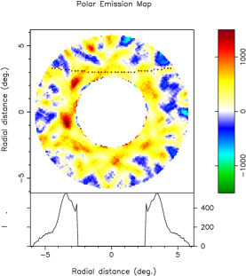
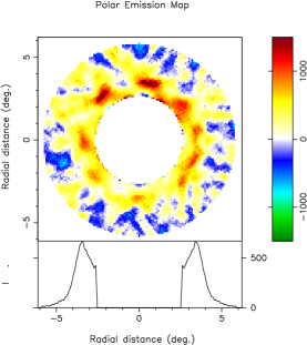
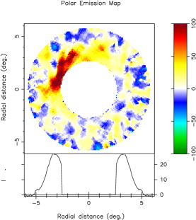
Figure 6: (Left) Average polar emission map for B0834+06 sequence-A made with 250 pulses. The sub-beams are less distinct and not equispaced, which contributes to the low Q-value of primary fluctuation. Considerable averaging has been carried out to improve the map’s signal-to-noise ratio. The string of dots at the top shows the track sampled by our sight-line. (Center) Average polar emission map for sequence B using $\sim 350$ pulses. The sub-beams intensities here show a systematic variation with azimuth, a property that manifested itself as the side-tones in the fluctuation spectra of this sequence. (Right) A map made using 64 pulses from sequence C. The streaky appearance results from inadequate sampling and/or averaging of the mapped region. Note the single prominent emission region and almost complete lack of emission over the rest of the polar region. The colour-scales used to display the intensities in the polar maps are shown on the right-side of respective maps. The apparent –ve intensities are a consequence of noise dominance in the off-pulse region.

7 Discussion

In the preceding sections we have presented our analysis of the fluctuation properties apparent in the decametric emission of pulsar B0834+06, as well as our efforts to understand the underlying emission pattern responsible for them.

B0834+06 is the only other pulsar (apart from B0943+10) for which we could estimate the circulation time of the polar emission pattern reliably using its fluctuation properties and viewing geometry. This estimation is based solely on our decameter observations. We have made polar emission maps from our 34.5 MHz sequences using the estimated $\hat{P}_{3}$ and drift direction, and those were presented in the earlier section. In carrying out our analysis, we followed a general strategy for the estimation of the circulation time of the polar emission pattern. This approach could be applied to other pulsars as well. We initially computed LRF- and HRF-spectra for this pulsar, and have shown that

• The primary modulation has a time delay between the two components of the star’s double profile.

• We argued that the amplitude fluctuations of the two components result from the ‘passage’ of the same emission entities as the polar emission pattern revolves progressively around pulsar’s magnetic axis. This, for the component separation of $50^{\circ}\!$ in magnetic longitude and the apparent modulation delay, suggested that the circulation time ($\hat{P}_{3}$) is  $\sim 14.9$ $P_{1}$.

• The HRF-spectrum, computed using set-B, exhibits sidebands around the primary modulation (see Fig. 2). These sidebands imply a slower periodicity modulating the primary modulation feature, having a period of $\sim 14.5\pm 0.8$ $P_{1}$. We notice discernible power in the LRF-spectrum of the same sequence (Fig. 1) at a frequency close to 0.073 c/$P_{1}$ (i.e. corresponding to a period of $\sim 14P_{1}$).

• The rewarding 64-pulse sequence (set-C) allowed a direct estimation of the circulation period, based on the low frequency feature in its fluctuation spectrum. This period estimate ($\sim 15P_{1}$) is consistent with the values determined from the other two sequences.

• We believe that these observations conclusively demonstrate the circulation time to be $\sim 14.9$ $P_{1}$.

• The estimates of the viewing geometry for this pulsar are uncertain. We carried out a search to refine the viewing geometry and other parameters of transform using the inverse of the cartographic transform. This search constrained the circulation time (now refined to be $\hat{P}_{3}$ = 14.84 $P_{1}$) and the drift direction of the pattern relative to the pulsar rotation, both of which are crucial for our mapping technique. However, $\alpha$ and $\beta$ were relatively poorly constrained in the case of this pulsar (B0834+06) and with this approach.

• A system of discrete sub-beams in steady rotation around the magnetic axis was found responsible for the observed pulse-to-pulse fluctuations. Because of the rather central traverse of the observer’s sightline, the circulation of the sub-beam system manifests as amplitude modulations, not as a subpulse drift.
  

The emission sub-beams of B0834+06 are discrete. They are not uniformly spaced in magnetic azimuth, and are irregular in form. The sub-beams appear to be wide in the radial direction, with $\Delta\rho/\rho\mathrel{\hbox{\hbox to0.0pt{\hbox{\lower 4.0pt\hbox{$\sim$}}\hss}\hbox{$>$}}}25\%$. We had concluded from our analysis of B0943+10 that the regions of radio emission correspond to a well-organized system of plasma columns. In B0834+06 we observe less order and more fluctuation in subbeam locations and brightness. This increased jitter in subbeam position, in addition to their non-uniform spacings, could result in the lower Q-values observed in the star’s fluctuation features. It was not possible to account for the null pulses, which could further affect the modulation $Q$.

We also made maps from successive subsections of the sequences and viewed them in a ‘movie’-like fashion. The variation, as noted above, in their relative locations and brightness is even more apparent within and across these maps. Although it is difficult to quantify these due to limited sensitivity, it is clear that usually only a couple of bright sub-beams seem to dominate the polar emission of this pulsar.

The isolated, bright emission patches close to the periphery appear due to a handful of strong pulses in our data and these areas receive negligible emission from a majority of the pulses. The origin of such intense pulses is unclear, however it may correspond to a Q-mode activity similar to that observed in pulsar B0943+10 (see paper-I).

The significance of our analysis also stems from the fact that pulsar B0834+06 is different from B0943+10 in its physical characteristics, its viewing geometry and hence in the nature of the apparent modulation it exhibits. The single-pulse fluctuations here mainly appear as modulations of its component amplitudes, unlike the drift patterns (or phase modulation) observed in B0943+10. Nonetheless we were able to relate such a general form of modulation to a well-defined rotating pattern in the polar emission region. This supports the picture that a set of discrete emitting sub-beams circulating within a hollow cone of emission, as envisioned in R&S, produces the single-pulse fluctuations in pulsars. The specific characteristics of the apparent fluctuations, e.g. whether it is an amplitude and/or phase modulation, would then depend mainly on the observer’s viewing geometry.

We now wish to quantitatively compare our current results as well as those obtained previously on B0943+10 with theoretical models. We tabulate all the relevant parameters of these two pulsars in Table 1, where the magnetic field estimates are derived from their timing behavior.

R&S express the circulation time of the discrete spark pattern as,

$$\hat{P}_{3}/P_{1}\,=K_{0}(B_{12}/P_{1}^{2}),$$ (6)

where $B_{12}$ is the average magnetic field (in units of 10${}^{1}2$ gauss) in the gap and $P_{1}$ is the pulsar rotation period in seconds. The constant $K_{0}$ (= 5.6 according to R&S) is considered to be a very shallow function of conditions local to the emission region.

Pulsar	$\alpha$	$\beta$	$B_{12}$	$P_{1}$	number of	$P_{3}$	$\hat{P}_{3}$ (R&S)	$\hat{P}_{3}$(G& S)	$\hat{P}_{3}$ (obs)	$\hat{P}_{3}$
				${\it s}$	sub-beams	(in ${\mathit{P}_{1}}$)	(in ${\mathit{P}_{1}}$)	(in ${\mathit{P}_{1}}$)	(in ${\mathit{P}_{1}}$)	(s)
B0943+10	$11^{\circ}\!.64$	$-4^{\circ}\!.31$	2	1.097	20	1.848	9.3	36.95	36.95	40.57
B0834+06	$30^{\circ}\!$	$-3^{\circ}\!$	3	1.273	8	1.855	13.1	103	14.84	18.9

Table 1: The various pulsar parameters for pulsars B0943+10 and B0834+06 are listed. We also compare between the observed circulation time and the theoretical estimates (see text).

From eq. 6 we write,

$$\left(\frac{({\hat{P}_{3}})_{0943+10}}{({\hat{P}_{3}})_{0834+06}}\right)_{estimated}=K\left(\frac{({\hat{P}_{3}})_{0943+10}}{({\hat{P}_{3}})_{0834+06}}\right)_{observed}$$ (7)

such that the parameter $K$ accommodates a possibility that $K_{0}$ in eq. 6 may not be a constant. K=1 would imply that the proportionality constant $K_{0}$ (irrespective of its precise value) in the eq. 6 remains unchanged from one pulsar to another. We, however, find the value of K to be 0.29. This suggests that $K_{0}$ is likely to have significant dependence on the pulsar parameters, particularly the estimated surface magnetic field and the inclination angle $\alpha$ (see Table 1). In order to meaningfully assess the exact nature of these and other possible dependences we would need $\hat{P}_{3}$ estimates to become available for several other pulsars.

Gil & Sendyk (2000; hereafter G&S) have advanced a modified-R&S spark model for radio pulsars. They have examined the estimates of subpulse drift and the details of polar emission maps from DR99 and paper-I. They claim to exactly reproduce such a behavior from their model, and the observations of B0943+10 allowed them to fix certain model parameters. We computed their predicted circulation time for B0834+06 given the parameters in Table 1. According to G&S model B0834+06’s circulation time should be $\sim 103\,P_{1}$ (for a “filling factor” of 0.1; and $\sim 78\,P_{1}$ for a filling factor computed according to their eq. 4), almost an order of magnitude higher than we have estimated from our observations. On the other hand, interestingly, the circulation time predicted B0834+06 based on the R&S model appears to be consistent with that observed. However, according to Gil, Melikidze & Geppert (2003; GMG2003) the original R&S derivation is in error (by a factor of 4, in $K_{0}$). The estimates for the circulation times in the two cases, based on their (i.e. GMG2003’s) recent detailed formulation of parameters associated with the ExB drift, show good agreement with those observed.

Our analyses were carried out using observations obtained at 34.5 MHz alone, and we do not have any polar emission maps made using single-pulse sequences at meter-wavelengths for comparison. We believe that such a structure of discrete sub-beams is valid even at higher frequencies. It would be possible to better account for the “null” pulses and their effect on the subbeam motion using the higher sensitivity of meter-wavelength data. Gil (1987) has reported the presence of strong orthogonal polarization modes (OPMs) in this pulsar. Hence, this pulsar may provide a useful context for studying possible causal relationships between the “null” pulses, OPMs and amplitude modulations.

8 Conclusions

Our observations of B0834+06 at 35 MHz show that the regular amplitude modulations observed in this pulsar are due to a system of discrete sub-beams rotating more or less steadily around the magnetic axis. This implies that the general amplitude modulations and regular “drifting subpulses” observed in some pulsars (e.g. Backer 1973) occur due to the same underlying reason. The nature of the modulation depends on the geometry; a shallow cut by the locus of the observer’s sightline leading to a conal single profile and subpulse drift, whereas a more central cut would lead to general amplitude modulations of the components of the average profile. The subbeam positions and intensities are not as stable as those observed in B0943+10 and we observed less order in our maps of B0834+06. We compared our estimates of the circulation time for pulsars B0834+06 and B0943+10 with the predictions of two specific theoretical models. We find that the models fail to predict the circulation time in a consistent manner for the two pulsars. Future similar data on other pulsars should help clarify possible dependences of circulation period on magnetic inclination angle and other parameters.

References

- [1] Asgekar, A. 2002, Ph. D. thesis, Indian Institute of Science, Bangalore.
- [2] Asgekar, A. & Deshpande, A. A. 1999, Bull. Astr. Soc. India, 302, 27
- [3] Asgekar, A. & Deshpande, A. A. 2000, ASP Conference Series, Vol. 202; Proc. of IAU Colloquium # 177, (San Francisco: ASP), Ed. M. Kramer, N. Wex, and R. Wielebinski, pp. 161
- [4] Asgekar, A. & Deshpande, A. A. 2001, MNRAS, 326, 1249 (paper-II)
- [5] Backer, D. C. 1973, ApJ, 182, 245
- [6] Deshpande, A. A. 2000, ASP Conference Series, Vol. 202; Proc. of IAU Colloquium # 177, (San Francisco: ASP), Ed. M. Kramer, N. Wex, and R. Wielebinski, pp. 149
- [7] Deshpande, A. A. & Radhakrishnan, V. 1994, JApA, 15, 329
- [8] Deshpande, A. A., Ramkumar, P. S., Chandrasekaran, S., Vinutha, C. & Prabu, T. 2004, in preparation.
- [9] Deshpande, A. A. & Rankin, J.M. 1999, ApJ, 524, 1008 (DR99)
- [10] Deshpande, A. A. & Rankin, J.M. 2001, MNRAS, 322, 438 (paper-I)
- [11] Deshpande, A. A., Shevgaonkar, R. K. & Sastry, Ch. V. 1989, JIETE, 35(6), 342
- [12] Drake, F. D., Craft, H. D., Jr. 1968, Nature, 220, 231
- [13] Gil, J. A. 1987, ApJ, 314, 629
- [14] Gil, J. A. & Sendyk, M. 2000, ApJ, 541, 351
- [15] Gil, J. A., Melikidze, G. I. & Geppert, U. 2003, A&A, 407, 315
- [16] Gupta, Y., Gil, J. A., Kijak, J. & Sendyk, M. 2004, A&A, 426, 229
- [17] Lyne, A. G. & Ashworth, M. 1983, MNRAS, 204, 519
- [18] Mitra, D. & Deshpande, A. A. 1999, A&A, 346, 906
- [19] Popov, M. V. & Sieber, W. 1990, Sov Astron, 34, 382
- [20] Rankin, J. M. 1986, ApJ, 301, 901
- [21] Rankin, J. M. 1993, ApJ, 405, 285
- [22] Rankin, J. M., Suleymanova, S. A. & Deshpande A. A. 2003, MNRAS, 340, 1076
- [23] Ritchings, R. T. 1976, MNRAS, 176, 249
- [24] Ruderman, M. A. & Sutherland, P. G. 1975, ApJ, 196, 51 (R&S)
- [25] Ruderman, M. A. 1976, ApJ, 203, 206
- [26] Slee, O. B. & Mulhall, P. S. 1970, Proc. ASA, 1, 322
- [27] Stinebring, D. R., Cordes, J. M., Rankin, J. M., Weisberg, J. M. & Boriakoff, V. 1984, ApJS, 55, 247
- [28] Sutton, J. M., Staelin, D. H., Price, R. M. & Weimer, R. 1970, ApJ, 159, L89
- [29] Taylor, J. H., Jura, M. & Huguenin, G. R. 1969, Nature, 223, 797
- [30] van Leeuwen, A. G. J., Stappers, B. W., Ramachandran, R. & Rankin, J. M. 2003, A&A, 399, 223