Radio Flares and the Magnetic Field Structure in GRB Outflows

Abstract

The magnetic field structure in gamma-ray burst (GRB) outflows is of great interest as it can provide valuable clues that might help pin down the mechanism responsible for the acceleration and collimation of GRB jets. The most promising way of probing this magnetic field structure is through polarization measurements of the synchrotron emission from the GRB ejecta, which includes the prompt $\gamma$-ray emission and the emission from the reverse shock. Measuring polarization in $\gamma$-rays with current instruments is extremely difficult: so far there is only one claim of detection (a very high degree of linear polarization in GRB 021206) which despite the favorable conditions remains highly controversial. The emission from the reverse shock that propagates into the ejecta as it is decelerated by the ambient medium peaks in the optical on a time scale of tens of seconds (the so called ‘optical flash’) and dominates the optical emission up to about ten minutes after the GRB. Unfortunately, no polarization measurements of this optical emission have been made to date. However, after the reverse shock finishes crossing the shell of GRB ejecta, the shocked ejecta cools adiabatically and radiates at lower and lower frequencies. This emission peaks in the radio after about one day, and is called the ‘radio flare’. We use VLA data of radio flares from GRBs to constrain the polarization of this emission. We find only upper limits for both linear and circular polarization. Our best limits are for GRB 991216, for which we find $3\;\sigma$ upper limits on the linear and circular polarization of $7\%$ and $9\%$, respectively. These limits provide interesting constraints on existing GRB models. Specifically, our results are hard to reconcile with a predominantly ordered toroidal magnetic field in the GRB outflow together with a ‘structured’ jet, where the energy per solid angle drops as the inverse square of the angle from the jet axis, that is expected in models where the outflow is Poynting flux dominated.

1. Introduction

The detection of linear polarization at the level of $\sim 1\%-3\%$ in the optical afterglow emission of several gamma-ray bursts (GRBs; see Covino et al., 2003, for a review) has been widely considered as a confirmation that synchrotron emission is the dominant radiation mechanism, at least in the afterglow stage. Synchrotron radiation is also believed to be the dominant emission mechanism in the prompt $\gamma$-ray emission and in the emission from the reverse shock, although the observational support for this is not as strong as for the afterglow. Soon after the first detection of linear polarization in the afterglow emission (Covino et al., 1999; Wijers, 1999) it has been realized that the temporal evolution of the polarization (both the degree of polarization $P$ and its position angle $\theta_{p}$) can probe the magnetic field structure in the emitting region, as well as the structure and the dynamics of GRB jets (Ghisellini & Lazzati, 1999; Sari, 1999).

While the polarization properties of the afterglow emission have received relatively wide attention (Loeb & Perna, 1998; Gruzinov & Waxman, 1999; Ghisellini & Lazzati, 1999; Sari, 1999; Medvedev & Loeb, 1999; Ioka & Nakamura, 2001; Granot & Königl, 2003; Rossi et al., 2004), the polarization of the prompt GRB emission received very little attention before the detection of a very high degree of linear polarization ($P=80\%\pm 20\%$) in the prompt $\gamma$-ray emission of GRB 021206 (Coburn & Boggs, 2003). Although this detection is highly controversial (Rutledge & Fox, 2004; Wigger et al., 2004), it has dramatically raised the interest in the polarization properties of the prompt emission. Two main explanations have been suggested for the production of tens of percent of polarization in the prompt $\gamma$-ray emission: (i) synchrotron emission from an ordered magnetic field in the ejecta (Granot & Königl, 2003; Coburn & Boggs, 2003; Lyutikov, Pariev & Blandford, 2003; Granot, 2003), and (ii) a viewing angle just outside the sharp edge of a jet, $\theta_{0}<\theta_{\rm obs}\lesssim\theta_{0}+1/\Gamma_{0}$ (Gruzinov, 1999; Waxman, 2003), where $\theta_{0}$ and $\Gamma_{0}$ are the initial half-opening angle and Lorentz factor of the jet, respectively. The second explanation can work with either synchrotron emission (Waxman, 2003; Granot, 2003; Nakar, Piran & Waxman, 2003) or inverse-Compton scattering of external photons (Shaviv & Dar, 1995; Eichler & Levinson, 2003; Lazzati et al., 2004a). In all the above cases, the polarization can be a good fraction of the maximal polarization for synchrotron emission, $P_{\rm max}\approx 60\%-70\%$.

The second explanation requires a narrow jet, $\theta_{0}\Gamma_{0}\lesssim{\rm a\ few}$, in order to have a reasonable probability of viewing the jet at an appropriate angle, $\theta_{0}<\theta_{\rm obs}\lesssim\theta_{0}+1/\Gamma_{0}$. Since a larger value of $\theta_{0}\Gamma_{0}$ is inferred for most GRBs (Panaitescu & Kumar, 2001a, b), this would imply little or no polarization in most cases, where our viewing angle is inside the jet, $\theta_{\rm obs}<\theta_{0}$. The first explanation, however, would imply a high polarization in all GRBs, if indeed they have a magnetic field that is ordered over angular scales $\gtrsim 1/\Gamma_{0}$.

The best way to reliably measure the polarization of the emission from the GRB ejecta is by using the emission from the reverse shock, which includes the optical flash and the radio flare. While no polarization measurements have been made so far in the optical flash, the polarization of the radio flare can be inferred from existing data. In §2 we discuss the existing candidates for radio flare emission in GRBs and the evidence that this emission is indeed from the reverse shock. In §3 we use archival data to derive upper limits on the linear and circular polarization of the radio flare emission, and in §4 we show that external propagation effects in the host galaxy or circumburst environment are not likely to cause a significant depolarization the radio emission. The upper limits on the polarization are contrasted with the predictions of different theoretical models in §5. In §6 we discuss propagation effects inside the source. We discuss the magnetic field configuration in the GRB ejecta in light of our results in §7 and give our conclusions in §8.

2. Is the Radio Emission from the Reverse Shock?

In order to draw conclusions regarding the magnetic field structure in the GRB ejecta from the polarization measurements of the radio flares, it is important to have some confidence that the radio emission is indeed from the original ejecta, whose electrons were heated by the reverse shock and then cooled adiabatically (Sari & Piran, 1999). The best candidates are GRBs 990123 (Kulkarni et al., 1999a), 991216 (Frail et al., 2000) and 020405 (Berger et al., 2003). A radio flare was also reported for GRB 970828 (Djorgovski et al., 2001), however in this case the source was detected in the radio at only one epoch and at one frequency, and there is no good evidence that suggests that this emission arises from the reverse shock. Also, the signal to noise in this case is rather bad, and does not give meaningful constraints on the polarization. Therefore, we shall concentrate on the other three GRBs for which there is better evidence that the radio flare emission is indeed from the reverse shock, and for which the quality of the data allows us to place interesting limits on the polarization.

In GRB 990123 the early radio emission (up to a day or two) has been found to agree very well with the expectations for the reverse shock emission (Sari & Piran, 1999; Kulkarni et al., 1999a; Nakar & Piran, 2004), especially when also taking into account the prompt optical emission from this GRB (Akerlof et al., 1999) which is also successfully explained as emission from the reverse shock. Furthermore, it is hard to explain the early radio emission as arising from the forward shock. Therefore, in GRB 990123 we have good reason to believe that the $8.46\;$GHz radio measurement at $t=1.25\;$days that is used in §3 to derive limits on the polarization was indeed dominated by emission from the reverse shock.

In GRB 991216 the radio emission in the first few days is inconsistent with the forward shock emission that is responsible for the optical and X-ray emission (Frail et al., 2000), and a different emission component is required. Frail et al. (2000) suggested either reverse shock emission, which naturally explains the early radio emission, or a two component jet model, where the early radio emission is from a spherical component with $E_{\rm iso}\sim 10^{54}\;$erg running into a very low external density, $n\sim 10^{-4}\;{\rm cm^{-3}}$. Such a low density is inconsistent with broad band afterglow fits to GRB 991216 (Panaitescu & Kumar, 2001a, b) which give a density higher by $\sim 4-5$ orders of magnitude. Also, the energy in the spherical component is very high, $\sim 10^{53}-10^{54}\;$erg, which is $\sim 2-3$ orders of magnitude higher than the values inferred for other GRBs (Frail et al., 2001; Panaitescu & Kumar, 2001b). Thus, the reverse shock is probably the best candidate for the early radio emission in GRB 991216, although it is hard to conclusively rule out other explanations.

In GRB 020405 the early rapid decay and spectral slope in the radio, $F_{\nu}\propto t^{-1.2\pm 0.4}\nu^{-0.3\pm 0.3}$, provide a reasonably good case that the early radio emission (within the first few days) is dominated by the reverse shock (Berger et al., 2003).

3. Limits on the Polarization from Radio Flares

We use archival VLA observations in order to measure the polarization of the radio flare emission discovered from GRBs to date. The VLA observations are typically short observations ($\sim$30 minutes) that were squeezed into the VLA schedule for these targets of opportunity. As such, there is insufficient calibration information from these short runs alone to allow for good polarization calibration in the standard manner using a calibrator observed over a wide range in parallactic angle. To overcome this difficulty we combined the VLA observations of the afterglows with calibration data taken from 1–4 days before or after the run. The instrumental leakage terms are stable on time-scales of months, so we are confident that an optimal calibration has been obtained. As a check, the polarization calibration was applied to the absolute flux calibrator observed on the same day as the radio flare (3C286 or 3C138), and the results were found to be consistent with their well-known properties.

We obtain only upper limits on the linear and circular polarization of three radio flares. Our results are summarized in Table 1. It is worth noting that so far only upper limits have been found for the radio polarization from GRB afterglows (Taylor et al., 2004, 2005). In the best case of the bright GRB 030329, the $3\;\sigma$ limits are $<$1% (Taylor et al., 2004).

Table 1Limits on the Polarization of Radio Flares in GRBs

GRB	$t$ (days)	$t_{j}$ (days)	$\Pi_{L}$	$\Pi_{C}$	$F_{\nu}$ ($\mu$Jy)
990123	1.25	$\approx 2$	$<23\%$	$<32\%$	$242\pm 26$
	1.49		$<11\%$	$<17\%$	$946\pm 56$
991216	2.68	$\sim 2$	$<9\%$	$<15\%$	$634\pm 26$
	1.49, 2.68		$<7\%$	$<9\%$	$715\pm 25$
020405	1.19	$\sim 1-2$	$<11\%$	$<19\%$	$492\pm 29$

Note. — The $3\;\sigma$ upper limits on the linear polarization, $\Pi_{L}=(Q^{2}+U^{2})^{1/2}/I$, and circular polarization, $\Pi_{C}=V/I$, of radio flares from GRBs, where $Q$, $U$, $V$ and $I$ are the Stokes parameters. In the third line for GRB 991216 we combine the two epochs from the first two lines in order to obtain a better limit on the polarization. These limits were derived using VLA observations at $8.46\;$GHz.

4. Propagation Effects External to the Source

Propagation effects might reduce the intrinsic linear polarization below detectable levels. A Faraday screen produced by ionized gas and magnetic fields can cause gradients in the observed polarization angle across the source, leading to depolarization if the intrinsic source size or the resolution element of the telescope is large compared to the gradients. The rotation measures (RM) can be related to the line-of-sight magnetic field, $B_{\|}$, by

$${\rm RM}=812\int\limits_{0}^{L}\left(\frac{n_{\rm e}}{1\;{\rm cm^{-3}}}\right)\left(\frac{B_{\|}}{\rm mG}\right)\left(\frac{dl}{\rm 1\;pc}\right)~{}{\rm rad\;m}^{-2}\ ,$$ (1)

where the upper limit of integration, $L$, is the distance from the emitting source to the end of the path through the Faraday screen along the line of sight. To produce a 90^∘ rotation at $8.4\;$GHz requires a RM of $1200\;{\rm rad\;m^{-2}}$.

In our Galaxy the RM can reach up to $\sim 1000\;{\rm rad\;m^{-2}}$ at very low Galactic latitudes, while at high Galactic latitudes it drops to a few$\,\times\,10\;{\rm rad\;m^{-2}}$ (Simard-Normandin, Kronberg & Button, 1981). At low Galactic latitudes Clegg et al. (1992) find a RM difference of up to $180\;{\rm rad\;m^{-2}}$ on scales of $1^{\circ}$ which translates to a linear scale of $\sim 100-200\;$pc and gradient of $\Delta{\rm RM}/\Delta L_{\perp}\sim 1\;{\rm rad\;m^{-2}\;pc^{-1}}$ in the RM. Since in our case the source size is $\sim(1-3)\times 10^{-2}\;$pc, this would correspond to a negligible rotation measure gradient across the image, $\Delta{\rm RM}\sim(1-3)\times 10^{-2}\;{\rm rad\;m^{-2}}$, some 5 orders of magnitude too low to cause significant depolarization. The host galaxies of GRBs are not thought to be greatly different from our own Galaxy (Bloom, Kulkarni, & Djorgovski, 2002).

Molecular clouds in our Galaxy typically exhibit variation of $\Delta{\rm RM}\sim 18-30\;\;{\rm rad\;m^{-2}}$ in the RM over scales of $\sim 2\;$pc (Wolleben & Reich, 2004). This corresponds to $\Delta{\rm RM}/\Delta L_{\perp}\sim 9-15\;{\rm rad\;m^{-2}\;pc^{-1}}$ and $\Delta{\rm RM}\sim 0.1-0.4\;{\rm rad\;m^{-2}}$ across the image, which is still some 4 orders of magnitude too low to cause significant depolarization. Individual Hii regions can produce enhanced RMs with dispersions of order $\sim 50\;{\rm rad\;m^{-2}}$ on scales of $\sim 0.2\;$pc (Gaensler et al., 2001), corresponding to $\Delta{\rm RM}/\Delta L_{\perp}\sim 250\;{\rm rad\;m^{-2}\;pc^{-1}}$ and $\Delta{\rm RM}\sim 2.5-7.5\;{\rm rad\;m^{-2}}$ across the image, which is still some 2-3 orders of magnitude too low.

Now we consider propagation effects in the immediate environment of the GRB, which was shaped by its progenitor. If the latter is a massive star, the immediate environment is the pre-explosion stellar wind which for a constant mass loss rate and wind velocity would give a density profile $n_{\rm ext}\propto R^{-2}$, at radii $R$ that are smaller than that of the wind termination shock. Such a density profile would imply a small deceleration radius $R_{\rm dec}$ and a very high density at that radius, which would in turn imply fast cooling of the reverse shock electrons and no detectable radio flare emission at $t\sim 1\;$day. Keeping this in mind, we shall assume a uniform external medium.

For GRB 020405, Berger et al. (2003) model the optical, X-ray and radio light curves with a uniform medium of density $n_{\rm ext}\sim 0.05\;{\rm cm^{-3}}$. Afterglow models applied to GRB 020405 predict an intrinsic diameter of the radio emitting region at 1.2 days after the burst of $\sim 10^{17}\;$cm. Values of the external density inferred from broad band afterglow modeling can be as high as $n\lesssim 30\;{\rm cm^{-3}}$ (Panaitescu & Kumar, 2001a, b; Yost et al., 2003). For GRB 990123 a very low density of $n_{\rm ext}\sim 10^{-3}\;{\rm cm^{-3}}$ is inferred, while for GRB 991216 the inferred density is more typical, $n_{\rm ext}\sim 5\;{\rm cm^{-3}}$.

Magnetic fields within the circumburst medium are not expected to cause a large depolarization, unless there is a clump with a high density contrast along our line of sight. A clump much smaller than the image size would have a small effect. A clump larger or comparable to the image size, $L_{\rm im}$, would produce a change $\Delta{\rm RM}$ in the rotation measure across the image which is roughly independent of the clump size, $L$, for a given density contrast $C$. This can be seen as follows. We have $n=Cn_{\rm ext}\propto C$ and assuming flux freezing and isotropic compression, $B\propto n^{2/3}\propto C^{2/3}$ so that ${\rm RM}\propto nBL\propto C^{5/3}L$, and the change in the RM across the image is roughly $\Delta{\rm RM}\sim{\rm RM}\times L_{\rm im}/L\propto C^{5/3}$, where the dependence on $L$ cancels out. Furthermore, the gradient in the rotation measure across the image would be comparable to the total rotation measure of a clump with a size similar to that of the image, $\Delta{\rm RM}\sim{\rm RM(L=L_{\rm im})}$, causing a relative rotation of the polarization position angle of

$$\frac{\Delta\theta_{p}}{90^{\circ}}\lesssim 0.45\left(\frac{n_{\rm ext}}{1\;{\rm cm^{-3}}}\right)\left(\frac{B_{\rm ext}}{10\;\mu{\rm G}}\right)\left(\frac{2R_{\perp}}{10^{17}\;{\rm cm}}\right)\left(\frac{C}{100}\right)^{5/3}\ ,$$ (2)

where $n_{\rm ext}$ and $B_{\rm ext}$ are the number density and magnetic field of the un-clumped external medium, and $R_{\perp}$ is the apparent radius of the image on the plane of the sky. Thus a clump with a density contrast $C\gtrsim 10^{2}$ and a size $\gtrsim 10^{17}\;$cm is required in order to induce significant depolarization. We also note that if such a clump lies within a distance of $\lesssim 1\;$pc from the progenitor star it would produce a detectable bump in the afterglow light curve, which was not observed for GRBs 990123, 991216 or 020405. Thus, such a clump along our line of sight seems unlikely. It is much less likely that such a clump would be along our line of sight in all the three GRBs that we analyzed.

Instead of a single clump, one might envision many small clumps with a covering factor of $f\sim 1$ (in order to cover most of the image). The typical clump size would have to be $L_{17}=L/(10^{17}\;{\rm cm})<1$ in order to avoid producing detectable bumps in the afterglow light curve. Since even for $C_{2}=C/100\sim 1$ we need $L_{17}\gtrsim 1$ in order for a single clump to produce significant depolarization (see Eq. 2), many small clumps are required along a random line of sight. If their rotation of the position angle would always be in the same direction, the required number of clumps would be $N_{0}\gtrsim C_{2}^{-5/3}L_{17}^{-1}$. However, since the direction of rotation of the position angle is expected to be random between different clumps, the total rotation would on average be zero with a mean r.m.s value of $N_{0}^{1/2}$ times that of a single clump. Thus a strong depolarization would require $\gtrsim N_{0}^{2}$ clumps along a random line of sight. Thus $N_{\rm cl}(R)L^{2}/R^{2}\gtrsim N_{0}^{2}\sim C_{2}^{-10/3}L_{17}^{-2}$ where $N_{\rm cl}(R)$ is the total number of clumps at radii $\sim R$. Thus the total mass in the clumps would be $\sim 0.1M_{\odot}(n_{\rm ext}/1\;{\rm cm^{-3}})C_{2}^{-7/3}L_{17}^{-1}R_{18}^{2}$ while there volume filling factor would be $\sim 0.1C_{2}^{-10/3}L_{17}^{-1}R_{18}^{-1}$. This means that the clumps would hold $\sim 10C_{2}^{-7/3}L_{17}^{-1}R_{18}^{-1}$ times more mass than that of the material between the clumps. Such an extreme clumping seems highly unlikely.

5. The Resulting Constraints on Theoretical Models

The radio flare emission typically peaks on a time scale of $\sim 1\;$day after the GRB. This is usually similar to the jet break time, $t_{j}$, in the afterglow light curve. At this time the Lorentz factor is typically $\Gamma\sim 10$, which is much smaller than its initial value, $\Gamma_{0}\gtrsim 100$. Thus a good part of the jet (or all the jet for $t>t_{j}$) is visible, and the observed polarization is an effective average value over this observed region. The optical flash emission peaks at the deceleration time $t_{\rm dec}$ when the Lorentz factor is close to its initial value (unless the reverse shock is highly relativistic), and should thus have a polarization close to that of the prompt $\gamma$-ray emission. It could therefore provide information that is complimentary to that from the radio flare.

The jet break time, $t_{j}$, plays an important role in the polarization light curve for most theoretical models. Therefore, it is important to know its value when comparing between theory and observations. In GRB 990123 there is a jet break in the optical light curve at $t_{j}\approx 2\;$days (Kulkarni et al., 1999b; Panaitescu & Kumar, 2001a). A similar jet break time, $t_{j}\approx 2\;$days, was found in the optical light curve of GRB 991216 (Halpern et al., 2000; Panaitescu & Kumar, 2001a) with a rather large uncertainty on this value. In GRB 020405 the jet break is not readily apparent in the data. Berger et al. (2003) deduce $t_{j}\approx 0.95\;$days from the fit to the broad band afterglow light curve, while Price et al. (2003) infer $t_{j}=1.67\pm 0.52\;$days. Thus we use a value of $t_{j}\sim 1-2\;$days for GRB 020405. In all cases the polarization limits are at times either similar to or slightly before the jet break time, $t\lesssim t_{j}$.

If the observed radio frequency is below the self absorption frequency, $\nu<\nu_{\rm sa}$, this can significantly reduce the polarization, for any magnetic field configuration. Nakar & Piran (2004) found that the peak of the radio flare emission is typically due to the passage of the self absorption frequency across the observed band. This would imply $\nu<\nu_{\rm sa}$ and a suppression of the polarization during the rise to the peak, and $\nu>\nu_{\rm sa}$ (no suppression of the polarization) during the decay after the peak. This can reduce the polarization before or around the time of the peak in the radio flare emission. In GRBs 991216 and 020405 the radio flux is decaying at the time of the measurement of the radio flare, and direct measurements of the spectral slope also support an optically thin spectrum ($\nu>\nu_{\rm sa}$), so that no suppression of the polarization is expected due to self absorption. For GRB 990123 the point used to measure the polarization seems to be near the peak of the radio flare and there is no good measurement of the spectral slope near this time. Thus the polarization might be somewhat suppressed if $\nu\lesssim\nu_{\rm sa}$, but probably not significantly suppressed since the relatively high flux and the proximity to the peak of the radio flare suggest that $\nu$ is not much smaller than $\nu_{\rm sa}$ and the two are at most comparable.

5.1. The Ejecta Dynamics after the Reverse Shock

Since the radio flare emission typically peaks at $t\lesssim t_{j}$, the possible lateral spreading of the jet at $t\gtrsim t_{j}$ can be neglected, and the jet dynamics can be reasonably approximated as being part of a spherical flow. After the passage of the reverse shock, the shocked external medium approaches the Blandford & McKee (1976, hereafter BM) self similar solution. However, the shocked ejecta has a significantly higher density than that given by the BM solution, and thus its rest mass density becomes comparable to its internal energy density (i.e. it becomes “cold”) much earlier on. For a mildly relativistic reverse shock this happens soon after the reverse shock crosses the shell, while for a relativistic reverse shock the shocked shell is first reasonably described by the BM solution, while it is still “hot”, but deviates from that solution once it becomes “cold” (Kobayashi & Sari, 2000).

For the BM solution the value of the self similar variable $\chi$ for a fixed fluid element, that is appropriate for the original ejecta, evolves with radius $R$ as $\chi=(R/R_{0})^{4-k}$ for an external density $\rho_{\rm ext}\propto r^{-k}$ (Granot & Sari, 2002), where $R_{0}$ is the radius where it crossed the shock, which for the original shell of ejecta is given by the deceleration radius, $R_{0}\sim R_{\rm dec}$. Also, $\gamma=\Gamma\chi^{-1/2}$ where $\Gamma\propto R^{-(3-k)/2}$ is the Lorentz factor of the fluid just behind the shock, so that $\gamma\propto R^{-(7-2k)/2}$ for the original ejecta. More generally one can assume some power law dependence of the Lorentz factor on radius, $\gamma\propto R^{-g}$, where the power law index $g$ can deviate from its value for the BM solution, $g=7/2-k$. This implies $t\propto R/\gamma^{2}\propto\gamma^{-(2g+1)/g}\propto$, $\gamma\propto t^{-g/(2g+1)}$ and $R\propto t^{1/(2g+1)}$.

Once the shell becomes “cold” (i.e. its rest energy exceeds its internal energy) its dynamics would deviate from the BM solution (Kobayashi & Sari, 2000), however, the power law index $g$ is still bounded by the value just behind the forward shock, $g=(3-k)/2$ (since the the ejecta shell is lagging behind the shocked external medium) and by the value for the BM solution, $g=7/2-k$ (since there is a larger inertia that resists the deceleration which is driven by a similar pressure). Thus, $(3-k)/2<g<7/2-k$ or $3/2<g<7/2$ for $k=0$ (a uniform density external medium).

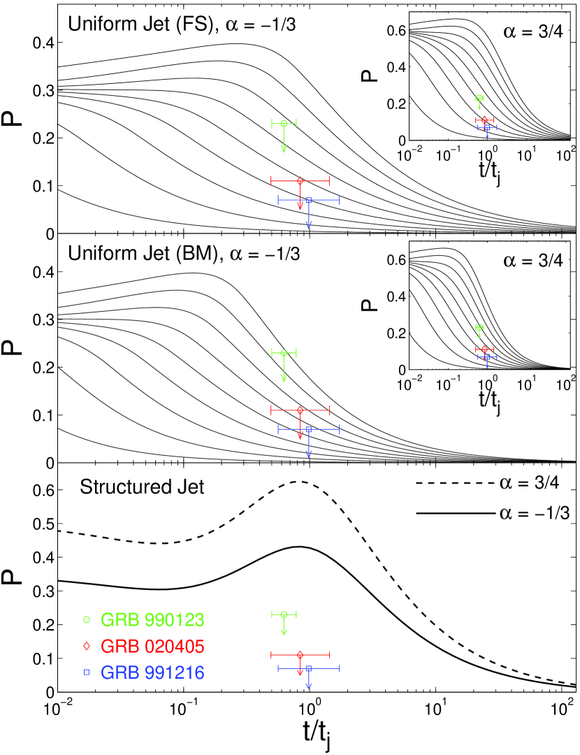
Figure 1.— Our $3\;\sigma$ upper limits for the linear polarization of the radio flare emission overlaid on the theoretical polarization light curves for a toroidal magnetic field in the GRB ejecta. The error bars represent the uncertainty in the determination of the jet break time $t_{j}$ from the optical afterglow light curve. The top two panels are for a uniform jet, and are calculated in Appendix A. The different lines, from top to bottom are for $\theta_{\rm obs}/\theta_{0}=0.9,\,0.8,\,...,\,0.1$. The main figure is for $\alpha=-d\log F_{\nu}/d\log\nu=-1/3$ and $P_{\rm max}=(\alpha+1)/(\alpha+5/3)=1/2$, while the inset is for $\alpha=3/4$ and $P_{\rm max}=21/29\approx 0.724$. In the top panel the Lorentz factor of the ejecta is assumed to remain equal to that of the freshly shocked fluid just behind the forward shock (FS), while the middle panel it is assumed to follow the Blandford & McKee (1976) (BM) self similar solution. The bottom panel is for a ‘structured’ jet where the energy per solid angle drops as $\theta^{-2}$ outside of some small core angle (taken from Lazzati et al., 2004b). In this case $P(t/t_{j})$ is practically independent of $\theta_{\rm obs}$.

At any given observed time $t>t_{\rm dec}$ the observed emission from the reverse shock is from a somewhat smaller radius and a slightly smaller Lorentz factor compared to the emission from the forward shock. This can be seen as follows. Let quantities normalized to their values at $t_{\rm dec}$ be denoted by a twiddle. From the equality of the observed time we have $\tilde{R}_{\rm RS}=\tilde{R}_{\rm FS}^{(4-k)/(2g+1)}=\tilde{R}_{\rm FS}^{(2g_{\rm FS}+1)/(2g_{\rm RS}+1)}$ where $g_{\rm FS}=(3-k)/2$ for the forward shock and $g=g_{\rm RS}$ for the reverse shock. Since $R\propto t^{1/(2g+1)}$ this implies that the ratio of the Lorentz factors for a fixed observed time is $\gamma/\Gamma=\tilde{R}_{\rm FS}^{-(g_{\rm RS}-g_{\rm FS})/(2g_{\rm RS}+1)}=\tilde{t}^{-(g_{\rm RS}-g_{\rm FS})/[(2g_{\rm RS}+1)(2g_{\rm FS}+1)]}=\tilde{t}^{-[g-(3-k)/2]/[(4-k)(2g+1)]}$. For $k=0$ this gives $\gamma/\Gamma=\tilde{t}^{-(g-3/2)/[4(2g+1)]}$ where the exponent ranges between $-1/16$ and $0$ for the possible range of $3/2<g<7/2$, which implies $\gamma/\Gamma\approx 1$. The somewhat smaller radius of the ejecta shell and the fact that it is typically cold by the time of the radio flare which is typically at $t\lesssim t_{j}$ suggest that a possible lateral spreading of the jet is probably not important for the radio flare emission, and thus it shall be neglected when calculating the polarization.

5.2. The Implications for Different Theoretical Models

If a high polarization in the prompt GRB is caused by a viewing angle $\theta_{0}<\theta_{\rm obs}\lesssim\theta_{0}+1/\Gamma_{0}$, then the polarization of the optical flash around its peak would be similar to that of the prompt $\gamma$-ray emission. This is since at this time ($t\sim t_{\rm dec}$) $\Gamma\sim\Gamma_{0}$ and $\theta_{j}\approx\theta_{0}$ (i.e. very little lateral expansion could have taken place before the deceleration time). However, at the time of the radio flare ($t\sim 1\;$day) $\Gamma\ll\Gamma_{0}$ and even a modest lateral expansion would give $\Gamma_{0}(\theta_{j}-\theta_{0})\gg 1$, so that the jet would occupy our line of sight. This could significantly reduce the polarization for a magnetic field that is random within the plane of the shock, as is expected to be produced in relativistic collisionless shocks by the two stream instability (Medvedev & Loeb, 1999). Furthermore, for a shock produced magnetic field the polarization of the radio flare should be similar to that of the optical emission from the forward shock, which is observed to be $P\lesssim 3\%$.

Such a low polarization suggests that the magnetic field is not random in 2D, fully within the plane the shock, but is instead more isotropic, and has a comparable component in the direction normal to the shock (Granot & Königl, 2003). Constraints similar to our best case, GRB 991216, for a larger number of GRB, could suggest a similar conclusion for the magnetic field in the ejecta.

Our upper limits on the polarization of the radio flare emission can put much tighter constraints on models where there is an ordered magnetic field in the GRB ejecta. If there is a magnetic field in the ejecta that is ordered over patches of angular scale $\theta_{B}\gtrsim 1/\Gamma_{0}$ then typically $P\sim P_{\rm max}$ during the prompt $\gamma$-ray emission and near the peak of the optical flash, while during the radio flare the polarization can be reduced due to averaging over $N\sim(\gamma\theta_{B})^{-2}$ incoherent patches, $P\sim P_{\rm max}\times\min[1,\gamma\theta_{B}]$ (Granot & Königl, 2003). This implies $\theta_{B}\lesssim P_{\rm lim}/\gamma P_{\rm max}$, where $P_{\rm lim}$ is our upper limit on the linear polarization. During the radio flare $\gamma\sim 10$ so that for GRB 991216 we have $P_{\rm lim}=0.07$ and $\theta_{B}\lesssim 1.4\times 10^{-2}(\gamma/10)^{-1}(P_{\rm max}/0.5)^{-1}\;$rad. In particular, if the magnetic field is roughly uniform over the whole jet ($\theta_{B}\sim\theta_{0}$) then this would imply $P\sim P_{\rm max}$ (Granot & Königl, 2003), i.e. tens of percent of polarization, which is definitely inconsistent with our upper limits.

For a toroidal magnetic field in the ejecta, we show our upper limits superimposed on the theoretical polarization light curves in Fig 1, both for a uniform jet and for a ‘structured’ jet. The latter is expected in models where the GRB outflow is Poynting flux dominated (Lyutikov, Pariev & Blandford, 2003; Lyutikov & Blandford, 2004). The polarization light curve for a structured jet is taken from Lazzati et al. (2004b). The polarization light curves for a uniform jet are derived in Appendix A. For a uniform jet we consider the two limiting cases for the evolution of the Lorentz factor of the ejecta after the deceleration time (see §5.1 for details): (i) the same as the forward shock Lorentz factor, and (ii) following the Blandford & McKee (1976) self similar solution. In case (ii) the Lorentz factor of the ejecta $\gamma$ decreases slightly faster with the observed time $t$ ($\propto t^{-7/16}$ instead of $t^{-3/8}$). This slightly ‘contracts’ the polarization light curve along the time axis. Also, while $\gamma\theta_{j}(t_{j})=1$ in case (i), we have $\gamma\theta_{j}(t_{j})=(t_{j}/t_{\rm dec})^{-1/16}\sim 0.65$ where typically $t_{j}/t_{\rm dec}\sim 10^{3}$, which shifts the polarization light curves to earlier times by a factor of $(t_{j}/t_{\rm dec})^{1/7}\sim 2.7$. This can be readily seen by comparing the upper and middle panels in Fig. 1.

Since $P_{\rm max}=(\alpha+1)/(\alpha+5/3)$ (Granot, 2003), a higher values of $\alpha$ produces a higher degree of polarization. Nevertheless, even their lowest values for optically thin synchrotron emission, $\alpha=-1/3$ and $P_{\rm max}=1/2$, still produce a fairly high degree of polarization.

For a uniform jet, $P(t\sim t_{j})$ significantly increases with $\theta_{\rm obs}/\theta_{0}$, and goes to zero at $\theta_{\rm obs}=0$. Thus, our upper limits on the polarization put upper limits on $\theta_{\rm obs}/\theta_{0}$. These limits also depend on the dynamical model for the GRB ejecta. For GRB 991216 we obtain $\theta_{\rm obs}/\theta_{0}\lesssim 0.4$ and $0.55$ for cases (i) and (ii), respectively.

The model that is most severely constrained by our upper limits on the polarization is a toroidal magnetic field together with a structured jet (see lower panel of Fig. 1). In this case all of our upper limits are significantly below the predictions of this model (by a factor of $\gtrsim 6$ for GRB 991216). Thus a predominantly toroidal magnetic field in the GRB ejecta together with a structured jet is hard to reconcile with our upper limits.

6. Propagation Effects at the Source

The effects of propagation in plasma inside the source on the synchrotron emission in GRBs has been recently considered (Matsumiya & Ioka, 2003; Sagiv, Waxman & Loeb, 2004, hereafter SLW04). In the early emission while the reverse shock is still going on, these effects can suppress linear polarization and produce up to tens of percent of circular polarization below the self absorption frequency $\nu_{\rm sa}$, for a magnetic field that is ordered on large scales (SLW04). We have obtained upper limits both on the linear polarization ($\Pi_{L}$) and on the circular polarization ($\Pi_{C}$) for the radio flare emission. The best limits are for GRB 991216: $\Pi_{L}<7\%$ and $\Pi_{C}<9\%$ ($3\;\sigma$). Our upper limits directly constrain such plasma propagation effects.

There are some arguments which suggest that plasma propagation effect should be relatively small and sub-dominant in the radio flare emission. First, the suppression of linear polarization and prevalence of circular polarization is much larger when the reverse shock electrons are fast cooling, i.e. most electrons cool significantly on a time scale smaller than the time it takes the reverse shock to cross the ejecta shell (SWL04), and is less significant when they are slow cooling (Matsumiya & Ioka, 2003). As mentioned in footnote 4, slow cooling is required in order to have a detectable radio flare emission, and is therefore the relevant case for us. Second, the effects of propagation in plasma decrease with time at a fixed observed frequency $\nu$ (Matsumiya & Ioka, 2003) and are significantly smaller at the time of the radio flare ($t\sim 1\;$day) compared to the time when the reverse shock is still going on ($t_{\rm dec}\sim 10^{2}\;$s). Furthermore, $\Pi_{L}<1\%$ is expected at $\nu>\nu_{\rm sa}$ (Matsumiya & Ioka, 2003), which seems to be the case for the radio flare emission that we consider in this paper.

Another related effect that might cause depolarization (SWL04) is a different amount of Faraday rotation for different frequencies at a given point on the image (which would be hard to resolve because of the finite instrumental spectral resolution) or at the same observed frequency between different points on the image (because of the different path lengths through the emitting plasma and different Doppler factor corresponding to different frequencies in the local rest frame of the emitting plasma). The $\Delta\nu/\nu$ which gives a Faraday rotation of $2\pi$ for a cold plasma is $|\Delta\nu/\nu|=\pi^{2}m_{e}^{2}c^{2}(\nu^{\prime})^{2}/(e^{3}n_{e}B^{\prime}W^{\prime})$ where $W^{\prime}$ is the width of the emitting region in the local frame (SWL04). For a relativistic plasma with a typical electron random Lorentz factor of $\gamma_{e}$ this expression should be multiplied by $\sim(\ln\gamma_{e})/\gamma_{e}^{2}$ (Matsumiya & Ioka 2003; SLW04) so that Faraday rotation and the resulting depolarization are suppressed. SWL04 consider fiducial parameters that result in fast cooling, and obtain that a significant depolarization is possible up to observed frequencies of $\nu\sim 10^{15}\;$Hz at $t\lesssim t_{\rm dec}$. Since we consider $\nu\sim 10^{10}\;$Hz and Faraday rotation scales as $\nu^{-2}$, we need to suppress Faraday rotation by some 10 orders of magnitude compared to their estimate.

Since a detectable radio flare requires slow cooling of the reverse shock, this would imply a smaller density and magnetic field in the local frame, which would reduce the Faraday rotation at $t\lesssim t_{\rm dec}$. Furthermore, SLW04 used $t_{\rm dec}=10\;$s while the radio flare occurs at $t\sim 10^{5}\;$s. We have $n_{e}W^{\prime}\propto R^{-2}$ and for the BM solution $W^{\prime}\propto R/\gamma\propto R^{9/2}$ and $B^{\prime}\propto 1/RW^{\prime}\propto R^{-11/2}$ so that $n_{e}B^{\prime}W^{\prime}\propto R^{-15/2}\propto t^{-15/16}$, which reduces the Faraday rotation by $\sim 4$ orders of magnitude between $t_{\rm dec}$ and the time of the radio flare. Also, at the time of the radio flare $\gamma\sim 5-10$ compared to $\sim 10^{2.5}$ at $t_{\rm dec}$ so that the same observed frequency corresponds to a higher frequency in the local rest frame of the emitting plasma ($\nu\approx\gamma\nu^{\prime}$). This reduces Faraday rotation by $\sim 3-4$ orders of magnitude. Finally, the reverse shock electrons must still be relativistic during the radio flare in order to emit the observed synchrotron radiation, and this will suppress the Faraday rotation by a factor of $\sim(\ln\gamma_{e})/\gamma_{e}^{2}$ (SWL04). Altogether, it seems that over a large part of the relevant parameter space there will not be significant depolarization of the radio flare emission due to different amounts of Faraday rotation at different points on the image, although it is hard to rule out some degree of depolarization for certain regions of parameter space.

7. discussion

If the magnetic field is carried out from the source, then at large radii it would be almost completely in the plane perpendicular to the radial direction, since the radial component of the magnetic field scales as $R^{-2}$ while the two transverse components scale as $R^{-1}$ if the magnetic field is initially tangled on small scales. If the flow and the magnetic field configuration are axially symmetric then $B_{\phi}\propto R^{-1}$ while $B_{\theta}\propto R^{-2}$ so that $B_{\phi}$ will dominate at large radii and the magnetic field will be toroidal. If the ratio of electromagnetic to kinetic energy is $\sigma\lesssim 1$, then the magnetic field is sub-dominant dynamically and the plasma can in principle keep it tangled on small scales within the plane normal to the radial direction, if it is initially tangled on such small scales, and its exact configuration is not obvious from theoretical considerations. For example, it could be ordered on angular scales $\theta_{B}\ll\theta_{j}$ where $\theta_{j}$ is the half-opening angle of the jet. On the other hand it might be ordered over the whole jet, possibly in a toroidal configuration. If, on the other hand, the GRB outflow is Poynting flux dominated (i.e. $\sigma\gg 1$) then the magnetic field is dynamically dominant and can move the plasma around and arrange itself in a toroidal configuration over the whole jet (Lyutikov & Blandford, 2003, 2004). Thus an ordered toroidal magnetic field is expected in the latter type of model.

These are the magnetic field configurations that are expected before the prompt gamma-ray emission. For $\sigma\lesssim 1$ the gamma-ray emission is likely due to internal shocks, which may cause a shock produced magnetic field that is expected to be random within the plane of the shock, so that it can add a random component to an initially ordered component. A similar effect can also occur in the reverse shock. The random component ($B_{\rm rnd}$) can reach values close to equipartition, so that it might be dominant over the ordered component ($B_{\rm ord}$) if the latter is well below equipartition ($\sigma\ll 1$). However, for $\sigma\sim 1$ with an initially ordered magnetic field, the shock produced random component can at most be comparable to the ordered component.

In Poynting flux dominated models, where initially $\sigma\gg 1$, there would be no reverse shock and therefore no radio flare if $\sigma$ remains $\gg 1$ after the prompt gamma-ray emission. Thus, in order to get a radio flare we need $\sigma\lesssim 1$. This might still be possible in such a model if after the dissipation of electromagnetic energy (magnetic reconnection) that causes the gamma-ray emission, the value of $\sigma$ decreases to $\sim 1$. Furthermore, the dissipation of magnetic energy (magnetic reconnection) that gives rise to the prompt gamma-ray emission in this type of models can also change the local configuration of the magnetic field in the emitting region, so that it might not be perfectly toroidal, and could also have a random component that could potentially be comparable in strength or possibly even exceed the ordered component.

A combination of an ordered and a random magnetic field component could decrease the resulting degree of polarization, compared to that for a purely ordered magnetic field, by a factor of $\sim\eta/(1+\eta)$ where $\eta\approx\langle B_{\rm ord}^{2}\rangle/\langle B_{\rm rnd}^{2}\rangle$ (Granot & Königl, 2003). Thus we obtain $\eta\lesssim 0.2$ for GRB 991216, where our upper limit on the polarization is $\gtrsim 6$ times smaller than the predicted value for a purely toroidal magnetic field. In other words, a sufficiently sub-dominant ordered toroidal magnetic field together with a larger random magnetic field component is required. This requirement is not trivial when starting from an ordered toroidal magnetic field close to the equipartition value, since the shock produced random field component would not exceed equipartition and thus would typically be at most comparable to the ordered component ($\eta\gtrsim 0.5$).

8. Conclusions

We have derived upper limits on the linear and circular polarization of the radio flare emission discovered from GRBs to date. Our results are summarized in Table 1. There is a reasonably good case that the radio flare emission in GRBs 990123, 991216, and 020405 indeed arises from the original ejecta that was shocked by the reverse shock and then cooled adiabatically (as discussed in §2). This emission is also most likely predominantly synchrotron radiation. Therefore, our upper limits on the polarization can be used to constrain the magnetic field structure in the ejecta of these GRBs.

Propagation effects outside of the emitting region might decrease the measured polarization below the value of the intrinsic polarization (see discussion in §3). We have demonstrated that the relatively small source size, $\lesssim 10^{17}\;$cm, at the time of the radio flare makes it very unlikely that gradients in the rotation measure across the image due to the magnetic field in the ISM of the host galaxy would cause significant depolarization. Depolarization due to a possible propagation in a molecular cloud or in the immediate circumburst medium might cause larger gradients in the rotation measure across the image, but still require extreme conditions in order to cause significant depolarization.

Propagation effects in the plasma inside the source might cause a different amount of Faraday rotation at different points on the image which may cause depolarization since the image is not resolved. For a fixed observed frequency, such a depolarization is much smaller during the radio flare compared to $t\lesssim t_{\rm dec}$ (see discussion in §6). Since Faraday rotation scales as $\nu^{-2}$ it might still be important in the radio for some parameter values, although it should not be very important for a large part of the relevant parameter space. Thus a more thorough investigation of this effect and its magnitude over the relevant parameter space is called for. Keeping this caveat in mind, we continue and examine the implications of our upper limits on the polarization under the assumption that there was no significant depolarization.

We have compared our upper limits to the predictions of different theoretical models. Models where the magnetic field is produced in the shock would in most cases produce a polarization below our upper limits. Furthermore, they are expected to produce a polarization similar to that of the afterglow emission, if indeed the dominant magnetic field in the afterglow is shock produced and if the magnetic field configuration behind the afterglow shock is similar to that behind the reverse shock. For lines of sight near the edge of the jet the expected polarization might in some cases exceed our upper limits, if the magnetic field behind the shock is maximally anisotropic (i.e. random within the plane of the shock or ordered in the direction normal to the shock). This might suggest a more isotropic magnetic field configuration behind the shock if comparable or better upper limits will be found in a larger sample of GRBs, similar to the current situation with the afterglow emission where linear polarization has been measured in several GRBs and was found to be $\Pi_{L}\lesssim 3\%$ in all cases, perhaps with one exception – GRB 020405 where a sharp spike in the polarization ($P=9.9\pm 1.3\%$ at $t=1.3\;$days) was reported (Bersier et al., 2003). We note that an almost simultaneous polarization measurement by a different group (Masetti et al., 2003) resulted in a significantly lower polarization, $P=1.5\pm 0.4\%$.

Our upper limits on the polarization put much stronger constraints on models in which there is an ordered magnetic field in the ejecta. A magnetic field that is roughly uniform across the whole jet would produce tens of percent of polarization, which is inconsistent with our upper limits. If the magnetic field is ordered over patches of angular scale $\theta_{B}$, which are mutually incoherent, then our upper limits on the polarization put upper limits on $\theta_{B}$. The tightest constraint is for GRB 9901216, for which we find $\theta_{B}\lesssim 10^{-2}\;$rad (see §5.2).

The polarization light curves for a toroidal magnetic field in the ejecta, together with our upper limits, are shown in Fig. 1. For a uniform jet, our upper limits on the polarization constrain our viewing angle toward GRB 991216 to be $\theta_{\rm obs}/\theta_{0}\lesssim 0.4-0.55$ where this range roughly covers the uncertainty in the dynamics of the ejecta at $t>t_{\rm dec}$ (as discussed in §5.2). These values are for a conservative value of the spectral slope, $\alpha=-1/3$ which corresponds to $P_{\rm max}=1/2$. For a structured jet with a toroidal magnetic field, $P\sim P_{\rm max}$ is expected at $t\sim t_{j}$ (which applies for all the upper limits given in Table 1). Therefore, this model appears to be inconsistent with our upper limits on the polarization.

Appendix A Polarization of a Uniform Jet with a Toroidal Magnetic Field

Here we derive the polarization of a uniform jet with an ordered toroidal magnetic field, by generalizing the results of Granot (2003) for a uniform transverse magnetic field. The emission is assumed to arise from a section of a thin spherical shell moving radially outward with a bulk Lorentz factor $\gamma\gg 1$, that lies within a cone of half opening angle $\theta_{j}$, which represents the jet. For simplicity, the emission is integrated over the jet at a fixed radius and the the differences in photon arrival time from different angles $\theta$ from the line of sight are ignored. An integration over the equal arrival time surface of photons to the observer might introduce small quantitative differences, but the results should be qualitatively similar, as we verified by comparing our results to those of Lazzati et al. (2004b). The emission in the local rest frame of the shell (where quantities are denoted by a prime) is taken to be uniform across the jet (hence a uniform jet), and depends only on the angle $\chi^{\prime}$ between the direction of the emitted radiation, $\hat{\bf n}^{\prime}$, and the local direction of the magnetic field, $\hat{\bf B}^{\prime}$. The polarization position angle at a given point on the jet makes an angle of $\theta_{p,B}=\phi+\arctan\{[(1-y)/(1+y)]\cot\phi\}$ from the local direction of the magnetic field, $\hat{\bf B}$ (Granot & Königl, 2003), where $y\equiv(\gamma\theta)^{2}$, and $\phi$ is the angle between $\hat{\bf B}$ and the direction from the line of sight to that point on the jet.

The Stokes Parameters are given by $(U,Q)/IP_{\rm max}=\int d\Omega I_{\nu}(\sin 2\theta_{p},\,\cos 2\theta_{p})/\int d\Omega I_{\nu}$, where $\theta_{p}$ is measured from some fixed direction, which for convenience we choose to be the direction from the jet symmetry axis to the line of sight. We have $d\Omega\propto d\varphi dy$ where $\varphi$ is the azimuthal angle around the line of sight measured from the direction between the jet axis and the line of sight. Let us use the notations $q\equiv\theta_{\rm obs}/\theta_{0}$, $y_{j}=(\gamma\theta_{j})^{2}$, $y_{\pm}=(1\pm q)^{2}y_{j}$, and $a\equiv\theta/\theta_{\rm obs}=q^{-1}(y/y_{j})^{1/2}$. We have $I_{\nu}=I^{\prime}_{\nu^{\prime}}(\nu/\nu^{\prime})^{3}$ with $I^{\prime}_{\nu^{\prime}}\propto(\nu^{\prime})^{-\alpha}(\sin\chi^{\prime})^{\epsilon}$, $\nu/\nu^{\prime}\approx 2\gamma/(1+y)$ and

$$\sin^{2}\chi^{\prime}=1-(\hat{\bf n}^{\prime}\cdot\hat{\bf B}^{\prime})^{2}\approx\left(\frac{1-y}{1+y}\right)^{2}\cos^{2}\phi+\sin^{2}\phi\approx\left(\frac{1-y}{1+y}\right)^{2}+\frac{4y}{(1+y)^{2}}\frac{(a+\cos\varphi)^{2}}{(1+a^{2}+2a\cos\varphi)}\ ,$$ (A1)

where $\hat{\bf n}^{\prime}$ is the direction in the local frame of a photon that reaches the observer. We also find that

$$\theta_{p}=\varphi-\arctan\left[\left(\frac{1-y}{1+y}\right)\frac{\sin\varphi}{(a+\cos\varphi)}\right]\ .$$ (A2)

From symmetry considerations $U=0$ and $P=|Q|/I$. The direction of the polarization vector on the plane of the sky is along the line connecting the jet symmetry axis and the line of sight. The degree of polarization is given by

$$\frac{P}{P_{\rm max}}=\left[\Theta(1-q)\int_{0}^{y_{-}}\frac{dy}{(1+y)^{3+\alpha}}\int_{0}^{2\pi}d\varphi(\sin\chi^{\prime})^{\epsilon}\cos 2\theta_{p}+\int_{y_{-}}^{y_{+}}\frac{dy}{(1+y)^{3+\alpha}}\int_{\Psi_{1}}^{2\pi-\Psi_{1}}d\varphi(\sin\chi^{\prime})^{\epsilon}\cos 2\theta_{p}\right]$$ (A3)

$$\times\left[\Theta(1-q)\int_{0}^{y_{-}}\frac{dy}{(1+y)^{3+\alpha}}\int_{0}^{2\pi}d\varphi(\sin\chi^{\prime})^{\epsilon}+\int_{y_{-}}^{y_{+}}\frac{dy}{(1+y)^{3+\alpha}}\int_{\Psi_{1}}^{2\pi-\Psi_{1}}d\varphi(\sin\chi^{\prime})^{\epsilon}\right]^{-1}\ ,$$

where $\Theta(x)$ is the Heaviside step function, $\cos\Psi_{1}=[(1-q^{2})y_{j}-y]/[2q(y_{j}y)^{1/2}]$, $P_{\rm max}=(\alpha+1)/(\alpha+5/3)$, and for producing the results shown in Fig. 1 we use $\epsilon=1+\alpha$ (Granot, 2003).

In order to produce polarization light curves a simple model of $\gamma(t)$ is added, where $t$ is the observed time. For a jet with no lateral spreading going into a uniform density medium $\gamma\propto t^{-\xi}$ where $\xi=3/8+(g-3/2)/[4(2g+1)]$ and $\gamma\propto R^{-g}$ (see §5.1). We identify the jet break in the optical light curve with $\Gamma\theta_{j}=1$ where $\Gamma$ is the Lorentz factor just behind the forward shock. Thus

$$y_{j}^{1/2}=\gamma\theta_{j}=\left(\frac{t_{j}}{t_{\rm dec}}\right)^{[g-(3-k)/2]/[(4-k)(2g+1)]}\left(\frac{t}{t_{j}}\right)^{-g/(2g+1)}\ .$$ (A4)

As discussed in §5.1 we have $(3-k)/2<g<7/2-k$. For the lower limit $g=(3-k)/2$ which corresponds to $\gamma=\Gamma$ we have $y_{j}=(t/t_{j})^{-(3-k)/(4-k)}$. For the upper limit $g=7/2-k$ we have $y_{j}=(t_{j}/t_{\rm dec})^{1/[2(4-k)]}(t/t_{j})^{-(7-2k)/[2(4-k)]}$.

References

- Akerlof et al. (1999) Akerlof, C. W., et al. 1999, Nature, 398, 400
- Berger et al. (2003) Berger, E., et al. 2003, ApJ, 587, L
- Bersier et al. (2003) Bersier, D., et al. 2003, ApJ, 583, L63
- Blandford & McKee (1976) Blandford, R. D., & McKee, c. F. 1976, Phys. Fluids, 19, 1130
- Bloom, Kulkarni, & Djorgovski (2002) Bloom, J. S., Kulkarni, S. R., & Djorgovski, S. G. 2002, AJ, 123, 1111
- Chevalier & Li (2000) Chevalier, R. A., & Li, Z. Y. 2000, ApJ, 536, 195
- Clegg et al. (1992) Clegg, A. W., Cordes, J. M., Simonetti, J. M., & Kulkarni, S. R. 1992, ApJ, 386, 143
- Coburn & Boggs (2003) Coburn, W., & Boggs, S. E. 2003, Nature, 423, 415
- Covino et al. (1999) Covino, S., et al. 1999, A&A, 348, L1
- Covino et al. (2003) Covino, S., et al. 2003, in ”Gamma Ray Bursts in the Afterglow Era” -3rd workshop, Rome 2002, ASP conf. ser., p. 169
- Djorgovski et al. (2001) Djorgovski, S. G., et al. 2001, ApJ, 562, 654
- Eichler & Levinson (2003) Eichler, D., & Levinson, A. 2003, ApJ, 596, L147
- Frail et al. (2000) Frail, D. A., et al. 2000, ApJ, 538, L129
- Frail et al. (2001) Frail, D. A., et al. 2001, ApJ, 562, L55
- Gaensler et al. (2001) Gaensler, B. M., Dickey, J. M., McClure-Griffiths, N. M., Green, A. J., Wieringa, M. H., & Haynes, R. F. 2001, ApJ, 549, 959
- Ghisellini & Lazzati (1999) Ghisellini, G., & Lazzati, D. 1999, MNRAS, 309, L7
- Granot (2003) Granot, J. 2003, ApJ, 596, L17
- Granot & Königl (2003) Granot, J., & Königl, A. 2003, ApJ, 594, L83
- Granot et al. (2001) Granot, J, Miller, M., Piran, T., Suen, W. M., & Hughes, P. A. 2001, in Gamma-Ray Bursts in the Afterglow Era, ed. E. Costa, F. Frontera, & J. Hjorth (Berlin: Springer), 312
- Granot & Sari (2002) Granot, J., & Sari, R. 2002, ApJ, 568, 820
- Gruzinov (1999) Gruzinov, A. 1999. ApJ, 525, L29
- Gruzinov & Waxman (1999) Gruzinov, A., & Waxman, E. 1999. ApJ, 511, 852
- Halpern et al. (2000) Halpern, J. P., et al. 2000, ApJ, 543, 697
- Ioka & Nakamura (2001) Ioka, K., & Nakamura, T. 2001, ApJ, 561, 703
- Kobayashi & Sari (2000) Kobayashi, S., & Sari, R. 2000, ApJ, 542, 819
- Kobayashi & Zhang (2003) Kobayashi, S., & Zhang, B. 2003, ApJ, 597, 455
- Kulkarni et al. (1999a) Kulkarni, S. R., et al. 1999a, ApJ, 522, L97
- Kulkarni et al. (1999b) Kulkarni, S. R., et al. 1999b, Nature, 398, 389
- Lazzati et al. (2004a) Lazzati, D., et al. 2004a, MNRAS, 347, L1
- Lazzati et al. (2004b) Lazzati, D., et al. 2004b, A&A, 422, 121
- Loeb & Perna (1998) Loeb, A, & Perna, r. 1998, ApJ, 495, 597
- Lyutikov & Blandford (2003) Lyutikov, M., & Blandford, R. D. 2003, in ”Beaming and Jets in Gamma-Ray Bursts”, Copenhagen, August 2002 (astro-ph/0210671)
- Lyutikov & Blandford (2004) Lyutikov, M., & Blandford, R. D. 2004, astro-ph/0312347
- Lyutikov, Pariev & Blandford (2003) Lyutikov, M., Pariev, V. I., & Blandford, R. D. 2003, ApJ, 597, 998
- Masetti et al. (2003) Masetti, N., et al. 2003, A&A, 404, 465
- Matsumiya & Ioka (2003) Matsumiya, M., & Ioka, K. 2003, ApJ, 595, L25
- Medvedev & Loeb (1999) Medvedev, M., & Loeb, A. 1999, ApJ, 526, 697
- Nakar, Piran & Waxman (2003) Nakar, E., Piran, T., & Waxman, E. 2003, JCAP, 10, 5
- Nakar & Piran (2004) Nakar, E., & Piran, T. 2004, MNRAS, 353, 647
- Panaitescu & Kumar (2001a) Panaitescu, A., & Kumar, P. 2001a, ApJ, 554, 667
- Panaitescu & Kumar (2001b) Panaitescu, A., & Kumar, P. 2001b, ApJ, 560, L49
- Price et al. (2003) Price, P. A., et al. 2003, ApJ, 589, 838
- Rossi et al. (2004) Rossi, E. M., Lazzati, D, Salmonson, J. D., & Ghisellini, G. 2004, MNRAS in press (astro-ph/0401124)
- Rutledge & Fox (2004) Rutledge, R. E., & Fox, D. B. 2004, MNRAS, 350, 1288
- Sagiv, Waxman & Loeb (2004) Sagiv, A., Waxman, E., & Loeb, A. 2004, ApJ, 615, 366
- Sari (1999) Sari, R. 1999, ApJ, 524, L43
- Sari & Piran (1999) Sari, R., & Pirn, T. 1999, ApJ, 517, L109
- Shaviv & Dar (1995) Shaviv, N. J., & Dar, A. 1995, ApJ, 447, 863
- Simard-Normandin, Kronberg & Button (1981) Simard-Normandin, M., Kronberg, P. P., & Button, S. 1981, ApJS, 45, 97
- Taylor et al. (2004) Taylor, G. B., Frail, D. A., Berger, E., & Kulkarni, S. R. 2004, ApJ, 609, L1
- Taylor et al. (2005) Taylor, G. B., Momjian, E., Pihlström, Y., Ghosh, T., & Salter, C. 2005, ApJ, submitted
- Waxman (2003) Waxman, E. 2003, Nature, 423, 388
- Wigger et al. (2004) Wigger, C., et al. 2004, ApJ in press (astro-ph/0405525)
- Wijers (1999) Wijers, R. A. M. J., et al. 1999, ApJ, 523, L33
- Wolleben & Reich (2004) Wolleben, M., & Reich, W. 2004, A&A, 427, 537
- Yost et al. (2003) Yost, S. A., Harrison, F. A., Sari, R., & Frail, D. A. 2003, ApJ, 597, 459