Chandra temperature profiles for a sample of nearby relaxed galaxy clusters

Abstract

We present Chandra gas temperature profiles at large radii for a sample of 13 nearby, relaxed galaxy clusters and groups, which includes A133, A262, A383, A478, A907, A1413, A1795, A1991, A2029, A2390, MKW4, RXJ1159+5531, and USGC S152. The sample covers a range of average temperatures from 1 to 10 keV. The clusters are selected from the archive or observed by us to have sufficient exposures and off-center area coverage to enable accurate background subtraction and reach the temperature accuracy of better than 20–30% at least to $r=0.4-0.5r_{180}$, and for the three best clusters, to $0.6-0.7r_{180}$. For all clusters, we find cool gas in the cores, outside of which the temperature reaches a peak at $r\sim 0.15\,r_{180}$ and then declines to $\sim 0.5$ of its peak value at $r\simeq 0.5r_{180}$. When the profiles are scaled by the cluster average temperature (excluding cool cores) and the estimated virial radius, they show large scatter at small radii, but remarkable similarity at $r>0.1-0.2r_{180}$ for all but one cluster (A2390). Our results are in good agreement with previous measurements from ASCA by Markevitch et al. and from Beppo-SAX by DeGrandi & Molendi. Four clusters have recent XMM-Newton temperature profiles, two of which agree with our results, and we discuss reasons for disagreement for the other two. The overall shape of temperature profiles at large radii is reproduced in recent cosmological simulations.

1. Introduction

Radial temperature profiles of the hot intracluster medium (ICM) in galaxy clusters and groups is one of the prime tools to study the gravitational processes responsible for large-scale structure formation and non-gravitational energy input into the ICM. The temperature profile is also an important cosmological measurement because in dynamically relaxed systems, it is the basic ingredient in estimating the total cluster mass distribution assuming hydrostatic equilibrium of the ICM. X-ray mass measurements at radius $r$ are only as accurate as $T$ and $dT/dr$ at that $r$ (e.g., Sarazin 1988).

Temperature measurements at large cluster radii are technically challenging. Cluster brightness at the virial radius is only 10% of the Cosmic X-ray Background (CXB) in the soft X-ray band, and a smaller fraction of the total (detector + CXB) background. The background spectrum is usually much harder than that of the cluster, leading to even lower surface brightness contrast at higher energies. The practical implication is that accurate spectral analysis near the virial radius is not possible, even with very long exposures, unless the background can be subtracted with better than 1% accuracy. Such accuracy is unachievable with past or present X-ray telescopes. The surface brightness contrast near 0.5 of the virial radius is higher, and the required accuracy of the background subtraction is $\sim 3\%$. This is easily achievable with Chandra (Markevitch et al. 2003) and marginally feasible with XMM-Newton (Nevalainen, Markevitch, & Lumb 2005).

Cluster observations with telescopes operating below the Earth’s radiation belts, such as ASCA and Beppo-SAX, are less affected by the background. However, poor point spread functions (PSF) of ASCA and Beppo-SAX, 1′–2′, was a major problem for temperature profile measurements. This problem is non-existent for Chandra and not a particular concern for XMM-Newton except in the cores of clusters with peaked surface brightness profiles (e.g., Markevitch 2002).

Table 1Cluster sample and Chandra observations

				Chandra observations
Cluster	$\langle T\rangle$	$z$	$N_{H}$  (*)	Aim point	Exposure, ksec	ACIS Mode	$r_{\text{max}}/r_{180}$	Comments
A133	4.2	0.057	$1.53\times 10^{20}\phantom{\,\,(*)}$	S+I	40+90	F+VF	0.67	$14^{\prime}$ offset in ACIS-I
A262	2.1	0.016	$8.10\times 10^{20}\,\,(*)$	S	30	VF	0.30	$\cdots$
A383	4.9	0.188	$3.92\times 10^{20}\phantom{\,\,(*)}$	I+I+S	20+10+20	VF	0.42	$\cdots$
A478	7.9	0.088	variable  (*)	S	43	F	0.60	$\cdots$
A907	5.9	0.160	$3.87\times 10^{20}\,\,(*)$	I	49+35+11	VF	0.58	$\cdots$
A1413	7.3	0.143	$2.19\times 10^{20}\phantom{\,\,(*)}$	I	10+113	VF	0.70	$\cdots$
A1795	6.1	0.062	$1.19\times 10^{20}\phantom{\,\,(*)}$	S+I	$7\times 15$	VF	0.53	Multiple offsets
A1991	2.6	0.059	$2.45\times 10^{20}\phantom{\,\,(*)}$	S	36	VF	0.48	$\cdots$
A2029	8.5	0.078	$3.04\times 10^{21}\phantom{\,\,(*)}$	S+I	87+9	F+VF	0.60	$\cdots$
A2390	8.9	0.230	$1.07\times 10^{21}\,\,(*)$	S	95	VF	0.90	$\cdots$
MKW4	1.6	0.020	variable  (*)	S	30	VF	0.39	$\cdots$
RXJ 1159+5531	1.9	0.081	$1.20\times 10^{20}\phantom{\,\,(*)}$	S	70	VF	0.38	$\cdots$
USGC S152	0.7	0.015	$1.55\times 10^{21}\phantom{\,\,(*)}$	S	30	VF	0.45	$\cdots$

      

      

      

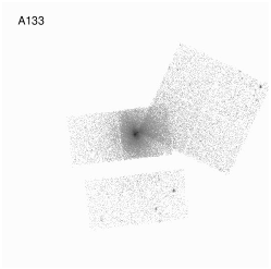
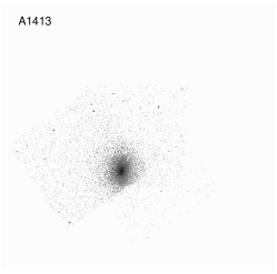
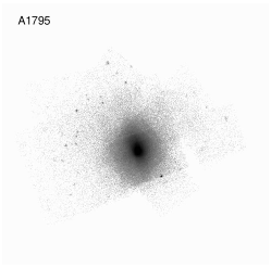
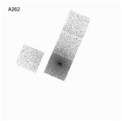
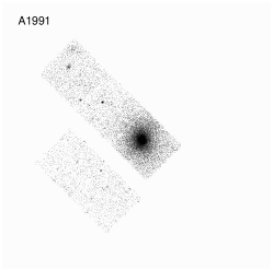
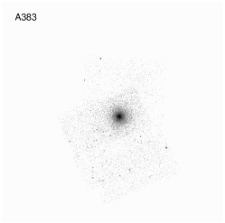
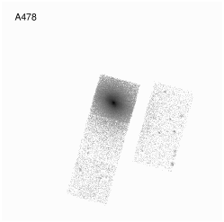
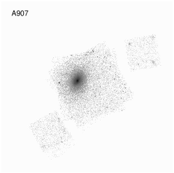
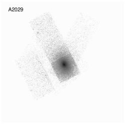
Figure 1.— Composite Chandra images in the 0.7–2 keV band. The images were not flat-fielded to indicate the difference in exposure coverage for different locations within the cluster. Each CCD chip is $\simeq 8^{\prime}$ on a side. North is up and East is to the left.

   

   

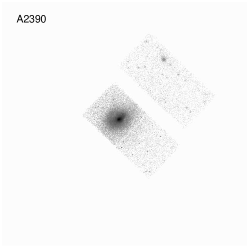
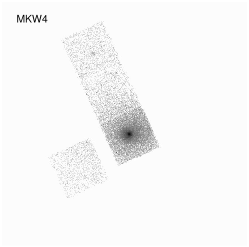
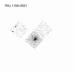
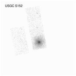
Figure 1.— continued.

Given the technical difficulties, early measurements of cluster temperatures at large radii have been controversial. ASCA was the first instrument with the necessary spectro-imaging capability. Cluster analysis was complicated by the complex PSF of the ASCA telescope, which if not taken into account, resulted in radially increasing apparent temperatures. Using ASCA data, Markevitch et al. (1996; 1998, hereafter M98; 1999) obtained temperature profiles for a sample of 32 nearby clusters, which showed significant declines with radius between $r=0.1-0.6\,r_{\rm vir}$ (hereafter, $r_{180}\equiv r_{180}$ from Evrard, Metzler & Navarro 1996). In clusters without obvious mergers, the radial temperature profiles outside the cool cores were similar when normalized to the virial radius. Consistent results were obtained, e.g., by Ikebe et al. (1997), Cannon et al. (1999) and Finoguenov et al. (2001). However, White (2000) found that most clusters in their large ASCA sample “are consistent with isothermality at the $3\sigma$ confidence level.” Some of the differences between White (2000) and other works can be attributed to White’s use of a PSF model that overestimated scattering at low energies. Also, White typically did not extend measurements to large radii because of large uncertainty inherent in his image deconvolution method, and in the overlapping radial range most of his temperature profiles are in fact consistent with M98.

Beppo-SAX was another instrument capable of spatially resolved spectroscopy; compared to ASCA, it had better PSF. Irwin & Bregman (2000) analyzed 11 clusters and reported isothermal or even increasing radial temperature profiles. However, De Grandi & Molendi (2002) pointed out a technical error in that work. Instead, De Grandi & Molendi found, in their analysis of 21 clusters, declining temperature profiles, in good agreement with M98 outside the cores ($r>0.15-0.2\,r_{\rm vir}$), although less peaked closer to the center. Similar profiles using Beppo-SAX data were obtained by Ettori et al. (2000) and Nevalainen et al. (2001).

Temperature profiles for individual clusters have been derived in the past few years using both Chandra and XMM-Newton observations. Previous Chandra results were mostly confined to the central region, typically within 0.2–0.3 virial radii (David et al., 2001; Schmidt, Allen & Fabian, 2001; Mazzotta et al., 2002; Sun et al., 2003a; Johnstone et al., 2002; Lewis, Buote & Stocke, 2003; Buote & Lewis, 2004; Sun et al., 2003b) although attempts were made to go to larger radii (Markevitch et al., 2000b; Markevitch & Vikhlinin, 2001). These measurements cannot be used to test the temperature decline at large radii observed by ASCA and Beppo-SAX. Published XMM-Newton temperature profiles extend to a larger fraction of the virial radius. Declining temperature profiles are observed in some clusters (Pratt & Arnaud, 2002; Takahashi & Yamashita, 2003; Zhang et al., 2004; Piffaretti et al., 2004; Belsole et al., 2005). However, there are also clusters reported to be isothermal at large radii (Majerowicz, Neumann & Reiprich, 2002; Pointecouteau et al., 2004; Belsole et al., 2004; Sakelliou & Ponman, 2004; Pratt & Arnaud, 2004). These lists include results for both relaxed clusters and major mergers, so some of the differences could be explained by the differences in the cluster dynamical state.

Chandra is well-suited for measurements of the temperature profiles to 0.5–0.6 of the virial radius thanks to its stable detector background, and fine angular resolution. In this paper, we present measurements of the temperature profiles to at least $\sim 0.4$ of the virial radius for a sample of 13 low-redshift clusters observed by Chandra with sufficiently long exposures that the statistical temperature uncertainties at this radius are reasonably small. The clusters are listed in Table 1. All these objects have a very regular overall X-ray morphology and show only weak signs of dynamical activity, if any. The main goal these observations was mass determination at large radii from the hydrostatic equilibrium equation. All of them have sufficient off-center area coverage to enable accurate background modeling and subtraction, which is the critical element of our analysis. Three clusters (A133, A907, A1413) were observed by us with a specific setup optimized for studying the outer regions. Even though the present cluster sample is not unbiased, it represents an essential step towards reliable measurements of the gas density and temperature profiles to a large fraction of the virial radius.

We assume $h=0.72$, $\Omega_{M}=0.3$, $\Omega_{\Lambda}=0.7$. Measurement uncertainties correspond to 68% CL.

2. Chandra data analysis

The nominal aim points (ACIS-I or ACIS-S) and exposure time for Chandra observations analyzed in this paper are listed in Table 1. Most of the observations were telemetered in VFAINT mode which provides for better rejection of the particle-induced background. In the case of ACIS-I pointings, we used the data from four ACIS-I chips for the temperature analysis, and S2 chip was generally used for monitoring the background. In the ACIS-S pointings, we used S3, S2, and available ACIS-I chips. The S1 chip was used mainly to monitor the background, but in low-redshift cool clusters (A262, MKW4, USGC S152), we used the S1 data also for the temperature profiles. In the rest of this section, we outline our Chandra data reduction procedures.

2.1. Calibration Corrections to Individual Photons

We start with “level 1” photon lists and apply standard processing using the CIAO tool acis_process_events. This includes correction for Charge Transfer Inefficiency (CTI; Townsley et al. 2000, Grant et al. 2004), re-computation of event grades, and detection of so-called afterglow events. We then remove photons detected in bad CCD columns and pixels and also those with bad ASCA grades (1,5,7). For observations telemetered in VFAINT mode, we apply additional background screening by removing events with significantly positive pixels at the border of the $5\times 5$ event island.

The next step is to compute calibrated photon energies. We apply updated ACIS gain maps and correct for its time dependence. Both corrections are available in the CIAO 3.1. The new gain maps are required for analyzing S1 data; improvements are very small for other chips.

The final step is to examine background light curves during each observation in order to detect and remove the flaring episodes. The flare detection was performed following the recommendations given in Markevitch et al. (2003). Clean exposure times are listed in Table 1.

2.2. Spectral Response Calibration

To take into account the spatial dependence of effective area and detector energy resolution, our analysis uses several important recent calibration advances outlined below.

ACIS optical blocking filters have been contaminated in-flight by a substance containing C, O, and F. Photoelectric absorption in the contaminant strongly reduces the low-energy effective area. Thanks to a number of calibration analyses, the properties of the contaminant are now known sufficiently accurately. The absorption spectrum of the contaminant has been measured using grating observations of bright AGNs with continuum spectra (Marshall et al., 2004). Time dependence of its thickness in ACIS-S was determined from the flux ratios of the calibration source lines. These corrections are built into CIAO since v3.0. New to our analysis is the inclusion of the spatial distribution of the contaminant. The center-to-edge difference of its optical depth is $\Delta\tau\simeq 0.5$ around 0.7 keV in both ACIS-I and ACIS-S arrays. Such variations, if unaccounted for, may have a major impact on the derived ICM temperatures. Recently, the spatial distribution of the contaminant has been measured accurately, so that the residual variations of the effective area are less than 3% at energies above 0.6 keV (Vikhlinin, 2004a). This correction was released to the Chandra users in October, 2004.

An additional non-uniformity of the CCD quantum efficiency arises because for a certain fraction of photons, the trailing charge produced by CTI makes them appear as charged particle-induced events, and they are screened out. Earlier calibration of this effect was based on a limited dataset and lacked an accurate model for its energy dependence. The resulting quantum efficiency residuals are $\simeq 5\%$ near $E=6\,$keV, marginally significant for the ICM temperature measurements. The new calibration released with CIAO 3.1 eliminates these residuals (Vikhlinin, 2004b).

The same CIAO release corrected an error in the CCD average quantum efficiency (QE) for the backside illuminated chips (S3 and S1) both at low and high energies (Edgar et al., 2004). This error, if neglected, results in a $\simeq 10\%$ mismatch in the temperature values determined from the back- (BI) and frontside illuminated (FI) chips. Temperature profiles spanning both types of chips would be affected.

Finally, the released calibration underestimates the effective area of the Chandra mirror by $\sim 10\%$ just above the Ir M edge, probably because the mirror surface is contaminated by a thin hydro-carbon layer (Marshall et al., 2003). We find that the corresponding effective area correction can be approximated by a “positive absorption edge”,

$$C=\exp(0.15(E/E_{0})^{-3})\quad\text{for $E>E_{0}$},$$ (1)

where $E_{0}=2.07$ keV. This correction reduces the best-fit temperatures by 5%. The expected effect of mirror contamination on the vignetting is negligible (D. Jerius, private communication). Corrections of the mirror area and updates to the QE of BI chips supersede the fudge factor of 0.93 that was suggested for the FI QE (Markevitch & Vikhlinin, 2001).

With all these recent calibration updates applied, the variations of the effective area within the Chandra field of view are modeled accurately to within 3%. This is verified directly by comparison of the A1795 spectra observed at different locations (Vikhlinin, 2004a), and indirectly by the agreement of the temperature profiles derived in different CCD chips.

2.3. Background Subtraction

As was discussed above, correct background subtraction is crucial for temperature measurements at large radii. The ACIS detector background can be modeled very accurately, to within 2% rms, which is one of the major advantages of Chandra over XMM-Newton for studying cluster outskirts.

The baseline background model can be obtained by using a compilation of the blank-field observations, processed identically to the cluster data, and “re-projected” onto the sky using the aspect information from the cluster pointing (see Markevitch et al. 2000 for a detailed description). This procedure results in background residuals of $\lesssim 10\%-20\%$ outside the obvious flaring periods. The accuracy can be significantly improved by small adjustments to the baseline model.

2.3.1 Quiescent Background

ACIS background above 2 keV is dominated by events from the charged particles. There are secular and short-term variations of the intensity of this component by as much as 30%, but its spectrum is very stable. Therefore, these trends can be accounted for by simply changing the background normalization. The renormalization factor can be derived for each observation using the data in the 9.5–12 keV band where the Chandra effective area is nearly zero and so all the observed flux is due to the background. Such a renormalization reduces the uncertainties in the modeling of the quiescent background to 2% rms, provided that flaring periods were screened out properly (Markevitch et al. 2003).

We extract and fit cluster spectra separately in the BI and FI chips, and flare filtering is also specific for each CCD type. Therefore, the background renormalizations were determined independently for these chip sets. A 2% scatter in the overall normalization per set per pointing was included in the overall temperature uncertainty budget. The accuracy of the quiescent background subtraction was verified using the spectra in the regions far from the cluster centers.

2.3.2 Soft Diffuse X-ray Background

In addition to the particle-induced background, the blank-field datasets contain the diffuse X-ray background. This component makes a large contribution to the total background below $\sim 1$ keV. The soft X-ray background was studied with Chandra by Markevitch et al. (2003) and XMM-Newton by Lumb et al. (2002). For most of the sky above the Galactic plane, the background spectrum is well represented by the MEKAL model with the Solar metallicity and $T\approx 0.2$ keV. A second component with $T\approx 0.4$ keV appears in locations where the diffuse flux is high. A fraction of the soft background is geocoronal in origin and variable in time (Wargelin et al. 2004). This component is dominated by the O VII and O VIII lines and its spectrum also can be approximated with sufficient accuracy by a thermal plasma model.

The blank-field datasets contain a typical mixture of the Galactic and geocoronal backgrounds. Since these components vary with location or time, the soft background in individual pointings is usually slightly different. Therefore, appropriate adjustments are needed, even though they rarely lead to qualitative changes in the derived temperature profile.

A certain fraction of the detector area in most of our observations was essentially free from the cluster emission and so we were able to determine the soft background adjustments in situ. We extracted spectra in those regions, subtracted the adjusted blank-field background (§2.3.1), and fit the residuals with an unabsorbed MEKAL model, whose normalization was allowed to be negative. The fit was performed in the 0.4–1 keV band because the soft background is usually dominated by the oxygen lines near 0.6 keV (Fig. 2). The derived adjustment is the real sky X-ray emission and is subject to the spatial variations in the effective area. Therefore, it must be included as an additional component in the spectral fits, with its normalization scaled by the region area. This approach was used before by, e.g., Markevitch & Vikhlinin (2001), and a similar method is used for XMM-Newton (e.g., Pratt et al. 2001, Majerowicz et al. 2002).

     

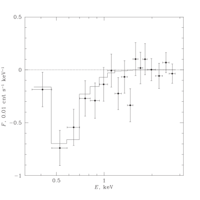
Figure 2.— The spectrum of the offset A133 pointing in the S2 chip with the nominal background subtracted. Residuals give an example of oversubtraction of the sky soft background. The fit is MEKAL model with negative normalization, Solar metallicity, and $T=0.18$ keV. It is included in the final background model.

The soft-band adjustments are within 20% of the nominal background flux in the 0.6–1 keV band in all our clusters, and do not qualitatively change the behavior of the temperature profiles in the radial range we consider. The only exceptions are A1991 and A2029 which are projected on the North Polar Spur. The soft background, if neglected, would have a serious impact on the derived temperature profiles in these cases. The statistical uncertainty in the normalization of this component is included in the uncertainties for the cluster temperatures.

Our adjustment procedure implicitly assumes that there are no significant fluctuations of the soft background on $\sim 15^{\prime}$ scales. We cannot test this assumption internally in each observation because cluster emission fills large fraction of the field of view. This is a limitation which can be addressed only by accurate mapping of the soft background in the vicinity of each cluster. However, we do not expect this to be a serious problem because the adjustments are usually small. In those cases with the high Galactic foreground flux, we have used the ROSAT All-Sky Survey maps to verify the absence of surface brightness gradients on relevant spatial scales.

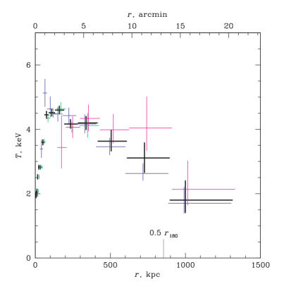
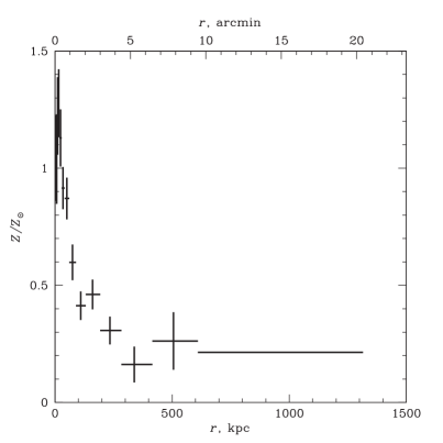
Figure 3.— Projected temperature and metallicity profiles for A133. The vertical bars are at the emission-weighted radius within each annulus. The independent temperatures measurements from S3 and FI chips in the ACIS-S pointing, and from ACIS-I pointing are shown in green, magenta, and blue, respectively. The values from the joint fit to these three datasets are shown in black. The metallicity at $r>600$ kpc was fixed at the average value from $r=270-600$ kpc, $Z=0.21$, and hence shown without the vertical error bars.

2.3.3 Subtraction of Readout Artifact

ACIS CCDs are exposed to the source during the readout cycle, which takes 41 ms or 1.3% of the nominal exposure time (3.2 s). This results in 1.3% of the source flux being uniformly re-distributed into a strip spanning the entire CCD along the readout direction, creating a “readout artifact”. This effect must be accounted when the readout artifact from the bright, central region contaminates the low surface brightness cluster outskirts. Fortunately, the readout artifact for sources without pile-up can be subtracted almost precisely, using a technique proposed by Markevitch et al. (2000a). A new dataset is generated with the CHIPY-coordinate of all the photons in the original observation randomized, and their sky coordinates and energies recalculated as if it were a normal observation. The obtained dataset is normalized by the ratio $41\,\text{ms}/3.2\,\text{s}$ and treated as an additional background observation. The normalization of the blank-field background is reduced by the same 1.3% to account for this subtraction. This correction was applied for all our clusters.

2.4. Spectral Fitting

The cluster spectra were extracted in annuli centered on the X-ray surface brightness peak, separately for each pointing and for FI and BI CCDs. The radial boundaries were chosen so that $r_{\text{out}}/r_{\text{in}}=1.5$ except for A262 where the statistical accuracy was sufficient to measure temperatures in narrower annuli, $r_{\text{out}}/r_{\text{in}}=1.33$. The spectra were fit in the 0.6–10 keV band to a single-temperature MEKAL model. The metallicity was allowed to be free in each annulus in the central region, where the statistical uncertainties were $\Delta Z<0.2$. At larger radii, metallicity was fixed at the average value in the last two radial bins where it was actually measured. If several datasets (pointings or FI/BI chips) contributed to the same annulus, they were fit jointly, with the spectral parameters (temperature, metallicity, Galactic absorption) tied and normalizations free for each dataset.

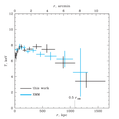
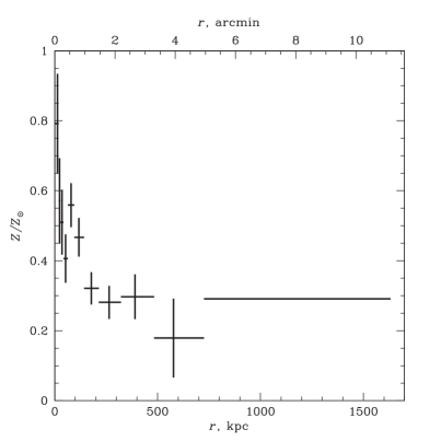
Figure 4.— Temperature and metallicity profiles for A1413. The blue error bars in the left panel show XMM-Newton results from (Pratt & Arnaud, 2002), renormalized by $+10\%$ to account for Chandra–XMM-Newton cross-calibration (see text).

Absorption was fixed unless a significant variation was found between the best-fit values in three cluster-centric annuli with radii 0–200, 200–400, and 400–800 kpc, where it usually could be measured accurately. Significant variations were detected only in A478 and MKW4. Furthermore, in most cases, the best-fit value of $N_{H}$ from the X-ray fit was consistent with the value from the radio surveys (Dickey & Lockman, 1990), and we used the latter in those cases.

3. Results for individual clusters

3.1. Abell 133

Abell 133 is a relaxed cluster at $z=0.057$ with the average temperature $T\simeq 4.5$ keV. It was observed by Chandra for 40 ksec in ACIS-S and for 90 ksec in the offset pointing in ACIS-I, which we have designed specifically for this measurement (Fig. 1). The X-ray image of A133 is nearly axially symmetric on large scales. The only detectable substructures are located within the central 40 kpc and likely caused by activity of the central AGN (Fujita et al. 2002)

The quiescent background had to be adjusted by $+5\%$ in the ACIS-I pointings, any by $-11\%$ and $-8\%$ in the ACIS-S pointing in the FI chips and BI chips, respectively. The spectrum extracted outside $20^{\prime}$ of the cluster center shows significant negative residuals around 0.6–0.7 keV, indicating that the soft X-ray background is over-subtracted. The residuals can be fit by the MEKAL model with $T=0.18$ keV and normalization corresponding to the 0.7–2 keV count rate $(-1.9\pm 0.3)\times 10^{-5}$ cnt s^-1 arcmin^-2. This component, with the normalization scaled by the area of the spectrum extraction region, is included in the cluster spectral fits.

Galactic absorption shows no statistically significant deviations and the cluster-average value from the X-ray fit, $N_{H}=(1.6\pm 0.4)\times 10^{20}$ cm^-2, agrees well with the radio value $1.53\times 10^{20}$ cm^-2, which was used thereafter.

The temperature and metallicity profiles are shown in Fig. 3. There is excellent agreement between the temperatures measured independently from the S3 and FI chips in the ACIS-S pointing (green and magenta, respectively), and from the off-set ACIS-I pointing (blue). We find similar agreement between different pointings and chips types in all our clusters.

The temperature values from the joint fits are shown by thick black error bars. There is a significant temperature decline at large radii, from $T=4.6\pm 0.15$ keV at $r=170$ kpc to $T=1.8\pm 0.6$ keV in the outermost annulus at $r\simeq 1000$ kpc. The upper limit on the temperature in this bin is 2.7 keV at the 90% CL. The temperature uncertainties quoted here and shown in Fig. 3 include uncertainties in the normalizations of the high-energy and soft background components, contributing $\pm 0.35$ and $\pm 0.1$ keV, respectively in the outermost bin.

The ICM metallicity is nearly Solar in the center and decreases to $Z\simeq 0.2$ at large radii. Similar metallicity profiles were derived from Beppo-SAX observations of several “cooling flow” clusters (De Grandi & Molendi, 2001). Chandra data cannot constrain the abundance outside $r=600$ kpc and so temperatures in this region are derived with the abundance fixed at $Z=0.21$, the average value for $r=270-600$ kpc. If, instead, one assumes that the observed abundance gradient continues at $r>600$ kpc, the best-fit temperatures will be only $\sim 3\%$ lower. The temperature variation with metallicity is much smaller than the statistical uncertainties for any $Z<0.5$, and we will ignore it for this and all other clusters.

Inside the central 70 kpc, we observe a sharp drop in the projected temperature, which is most likely caused by radiative cooling. Interestingly, there is also a spike in metallicity within this radius. Such behavior is observed in all our clusters. However, we note that a reliable metallicity analysis in the central regions, where the temperature gradients are strong, requires spectral deprojection. This is beyond the scope of this work, since we are primarily interested in the temperature profiles at large radii. Our values of the metallicity in the very centers should be treated with caution.

3.2. Abell 1413

Abell 1413 ($z=0.1429$) was observed in three pointings. One observation (OBSID 537) was almost entirely affected by a background flare and it was discarded from the analysis. The composite image from the remaining two observations is shown in Fig. 1. The cluster center was placed in the I3 chip in the shorter observation (OBSID 1661, 10 ksec). In the longer observation (OBSID 5003, 75 ksec), the cluster center was deliberately placed off-axis in the I2 chip to obtain better coverage for the outer regions. Since the exposure times are very different, our results are dominated by the data from OBSID 5003. The X-ray image is elongated in the North–South direction. However, no obvious signatures of a merger are observed, except for a weak edge in the surface brightness at 400 kpc North of the cluster center.

We do not detect any radial variations in the Galactic absorption, and the averaged value from the X-ray spectral fit, $N_{H}=(2.4\pm 0.8)\times 10^{20}$ cm^-2, is consistent with the radio value, $2.19\times 10^{20}$ cm^-2. The spectrum from $r>1700$ kpc shows negative residuals near 0.6 keV, therefore the soft background is over-subtracted. The corresponding background correction can be modeled with the MEKAL spectrum with $T=0.20$ keV and normalization corresponding to the 0.7–2 keV count rate $(-2.7\pm 0.2)\times 10^{-5}$ cnt s^-1 arcmin^-2.

The projected temperature and metallicity profiles are shown in Fig. 4. The results are qualitatively similar to A133 — there is a temperature drop by a factor of $\sim 2$ in the outermost bin. There is also a cool region within the central 100 kpc associated with a spike in the metallicity profile.

A1413 is one of the clusters with the most accurately measured XMM-Newton temperature profiles (Pratt & Arnaud, 2002). Comparison with our results is obviously in order. The average XMM-Newton temperature of the cluster is $\approx 10\%$ lower than our measurements. A similar difference is observed in distant clusters (Kotov & Vikhlinin, in preparation), and therefore most likely reflects cross-calibration problems. This difference is unimportant for comparison of the temperature gradients and we uniformly renormalized the XMM-Newton values by $+10\%$. The corrected XMM-Newton temperature profile is shown by blue error bars in Fig. 4. There is excellent agreement between the Chandra and XMM-Newton measurements, except in the very center where XMM-Newton can be affected by poorer angular resolution.

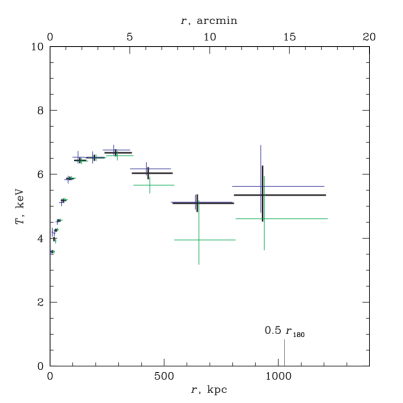
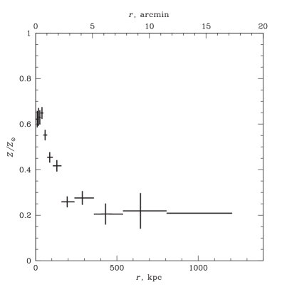
Figure 5.— Temperature and metallicity profiles for A1795. Independent $T$ measurements from the BI and FI chips are shown by green and blue, respectively.

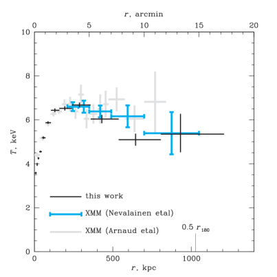
Figure 6.— Comparison of Chandra and XMM-Newton temperature profiles for A1795. The XMM-Newton results from Arnaud et al. (2001) are shown in grey. The same observation was also analyzed by Nevalainen et al. (2004; blue error bars with caps). Note that XMM-Newton values were renormalized by $+10\%$ to account for cross-calibration (see § 3.2).

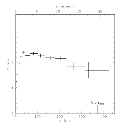
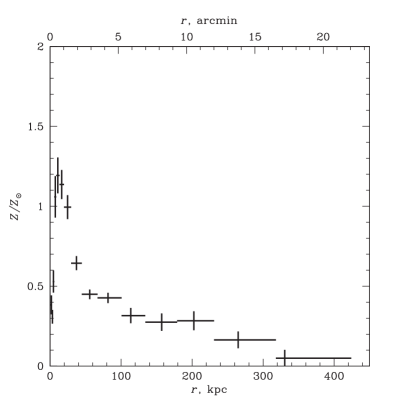
Figure 7.— Temperature and metallicity profiles for A262.

3.3. Abell 1795

Abell 1795 ($z=0.0622$), was observed by Chandra multiple times, within the Guaranteed Time program in 1999 and early 2000, and subsequently in 6 pointings as a calibration target. We do not use the 1999 observation (OBSID 494) because accurate gain calibration is still unavailable for that time period. The remaining 7 pointings, in which the cluster was placed at different locations within the S3 and I3 chips, have a combined exposure of more than 100 ksec (Fig. 1).

There is no significant variation of Galactic absorption with radius, and the cluster-average value, $N_{H}=(1.35\pm 0.12)\times 10^{20}$ cm^-2, is consistent with the value from the radio surveys, $1.19\times 10^{20}$ cm^-2. We do not detect any signatures of incorrect subtraction of the soft background at the largest radius covered by Chandra pointings. Therefore, no additional background correction is done, but a typical uncertainty in normalization of such a component (see discussion on A133 and A1413 above) is still included in the final error budget.

The temperature and metallicity profiles are shown in Fig. 5. There is a significant temperature decrease at large radii relative to the temperature just outside the central cool region. The temperature drop is weaker than that in A133 and A1413, but we note that Chandra observations of A1795 cover a smaller fraction of the cluster virial radius.

Multiple observations of A1795 at different locations on the detector make this cluster an ideal case for testing the calibration uncertainties. The temperatures derived independently from the data in the BI and FI chips are shown in Fig. 5 by green and blue error bars, respectively. There is excellent agreement, even though these datasets are from CCDs with substantially different quantum efficiencies, and the data at the same distance from the cluster center sample different detector regions and therefore different contamination depths.

Temperature profile for A1795 was the first one published from XMM-Newton (Arnaud et al., 2001). XMM-Newton results are compared with our measurements in Fig. 6. No obvious trend for the temperature to decline with radius is suggested by the Arnaud et al. analysis (grey error bars), but the difference with our results is within their statistical uncertainties. A subsequent reanalysis of the same XMM-Newton data by Nevalainen et al. (2004), who performed a more rigorous background flare exclusion, produced a temperature profile fully consistent with our results (blue error bars with caps).

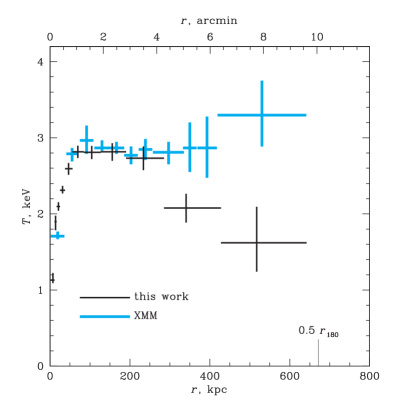
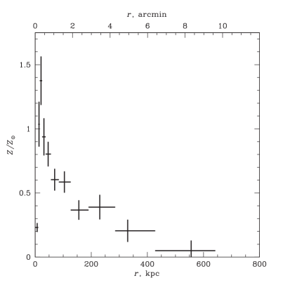
Figure 8.— Temperature and metallicity profile for A1991. XMM-Newton results from Pratt & Arnaud (2004) are shown in blue. Note that XMM-Newton values were renormalized by $+10\%$ to account for cross-calibration (see § 3.2).

3.4. Abell 262

Abell 262 ($z=0.0162$, $T\simeq 2$ keV) was observed in ACIS-S for 30 ksec. The X-ray image (Fig. 1) on large scales in nearly symmetric, but there is substructure in the very central region, probably related to past activity of the central radio source (Blanton et al., 2004). We include data from the S1 chip in this observation. This CCD is not used for temperature measurements in hot clusters, because its particle-induced background is very high above 5 keV, but S1’s performance is comparable to that of S3 for clusters with $T\lesssim 2$ keV, such as A262.

We do not find any problems with the soft background subtraction in the A262 observation. The cluster brightness is sufficiently high everywhere in the field of view and therefore any reasonable background variations have negligible effect on the derived temperatures. The best-fit Galactic absorption is constant with radius within the measurement uncertainties but its average value, $N_{H}=(8.1\pm 0.3)\times 10^{20}$ cm^-2 is significantly higher than the radio value, $5.4\times 10^{20}$ cm^-2. Excess absorption in this cluster was also found in the ROSAT data (David, Jones, & Forman, 1996). David et al. demonstrated that the excess absorption can be fully explained by intervening Galactic cirrus visible in the IRAS $100\,\mu$ image. We use the best-fit X-ray value of $N_{H}$ in the further analysis.

The temperature and metallicity profiles of A262 are shown in Fig. 7. Note a strong central spike of metallicity, which coincides with the temperature decrement within the inner 50 kpc. There is a significant temperature decrease at $r>100-200$ kpc. Note that in this case, we use a very different portion of the ACIS energy band for the temperature determination and so systematics should be very different from those in the hotter clusters. It is reassuring, therefore, that we observe a qualitatively similar temperature structure.

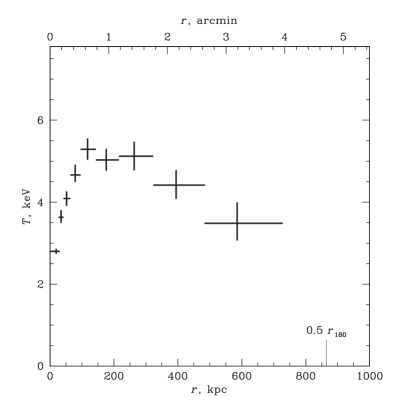
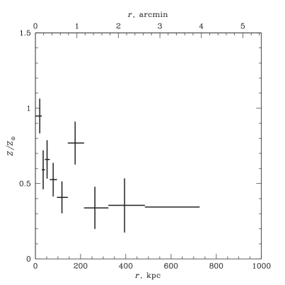
Figure 9.— Temperature and metallicity profiles for A383.

3.5. Abell 1991

Abell 1991 is a $T\simeq 2.8$ keV cluster at $z=0.0592$ and its virial radius fits almost entirely within the Chandra field of view. A1991 was observed for 40 ksec in ACIS-S (Fig. 1). Sharma et al. (2004) report substructure within the central $10^{\prime\prime}$ but otherwise, the X-ray image is very symmetric.

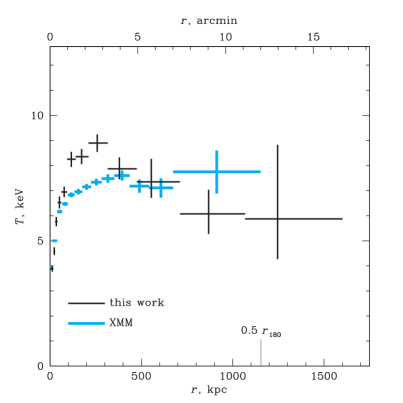
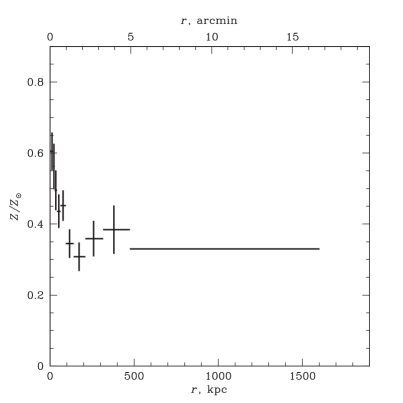
Figure 10.— Temperature and metallicity profiles for A478. The XMM-Newton measurements (renormalized by $+10\%$, see § 3.2) are shown in blue.

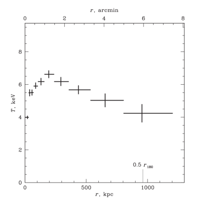
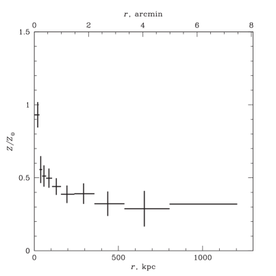
Figure 11.— Temperature and metallicity profiles for A907.

Absorption, derived from the X-ray spectra, is constant with radius and consistent with the radio value, $N_{H}=2.45\times 10^{20}$ cm^-2. The cluster is projected on the North Galactic Spur and in this field there is a strong excess flux at low energies. Fortunately, the spectrum and normalization of this soft background component can be determined from the same observation because the Chandra’s field of view extends to $20^{\prime}$ from the cluster center, where the object surface brightness is negligible. Galactic foreground was measured independently from the 0.4–1.5 keV spectra in the $9.5^{\prime}-14.5^{\prime}$ and $14.5^{\prime}-20^{\prime}$ radial ranges extracted in the S1 and ACIS-I chips. The excess flux requires two components with different $T$, similar to results for the Chandra blank fields in the Spur area (Markevitch et al., 2003). The best-fit temperatures are $T_{1}=0.157\pm 0.029$ keV and $T_{2}=0.51\pm 0.15$ keV, and relative emission measures are $K_{2}/K_{1}=0.285$. The normalization corresponds to a flux of $2.45\times 10^{-16}$ erg s^-1 cm^-2 per arcsec² in the 0.4–1.5 keV energy band. The normalizations are consistent in all four spectra, indicating that this soft component indeed represents a uniform foreground and is not related to the cluster.

The temperature and metallicity profiles of A1991 are shown in Fig. 8. The spectrum in the innermost bin clearly requires several temperature components and therefore the derived metallicity for a single-temperature fit is artificially low.

XMM-Newton results for A1991 were recently published by Pratt & Arnaud (2004). They derive an essentially isothermal profile, which disagrees with our results at $r>300$ kpc at a $\sim 3\sigma$ confidence level (blue points in Fig. 8). The difference in modeling of the excess soft background in this field and background flares are obvious suspects for the discrepancy between the XMM-Newton and Chandra results; unfortunately, Pratt & Arnaud do not provide information necessary for a more detailed comparison.

3.6. Abell 383

Abell 383 ($z=0.1883$) was observed with Chandra in 3 pointings, for 20 and 10 ksec in ACIS-I, and for 20 ksec in ACIS-S (Fig. 1). There are faint extended X-ray sources in the X-ray surface brightness at $5.5^{\prime}$ to the South-East and at $\sim 7^{\prime}$ to the North-West, probably related to infalling subgroups. They were excluded from the radial profile analysis.

Galactic absorption derived from the X-ray spectra is constant with radius and consistent with the radio value, $3.92\times 10^{20}$ cm^-2. The spectrum extracted in the outermost regions of the field of view shows negative residuals near 0.6 keV, similar to those in the A133 observation (Fig. 2). The residuals can be fit with the MEKAL model with $T=0.18$ keV and a negative normalization corresponding to a 0.7–2 keV count rate of $(-1.5\pm 0.3)\times 10^{-6}$ cnt s^-1 arcmin^-2. This component was included in the spectral fits. The temperature and abundance profiles for A383 are shown in Fig. 9.

3.7. Abell 478

Abell 478, one of the highest-temperature clusters in our sample, was observed in ACIS-S for 43 ksec (Fig. 1). In the central $30^{\prime\prime}$ there is substructure associated with activity of the central AGN but otherwise, the cluster is symmetric. Chandra analysis of the central $4^{\prime}$ was presented by Sun et al. (2003a). Our analysis supersedes the temperature profile in that paper because we use updated calibrations. This cluster was also studied by XMM-Newton (Pointecouteau et al., 2004).

The spectra from the outermost regions of the field of view, which are almost free from cluster emission, do not show any significant residuals in the soft band. However, there are significant variations in the Galactic absorption. The best-fit $N_{H}$ changes linearly with radius from $(3.09\pm 0.09)\times 10^{21}$ cm^-2 at $r=0$ to $(2.70\pm 0.06)\times 10^{21}$ cm^-2 at $r=4^{\prime}$; these are significantly in excess of the radio value, $1.51\times 10^{21}$ cm^-2. At $r>5^{\prime}$, $N_{H}$ drops quickly, reaching $1.5\times 10^{21}$ cm^-2 at $r\approx 8^{\prime}$ and stays constant at larger radii. Pointecouteau et al. obtained very similar results from the XMM-Newton data and argued that the excess absorption is most likely caused by a Galactic dust cloud projected on one side of the cluster, including the center. Since absorption is a strong function of radius in this case, we leave it free in all spectral fits. The absorption distribution may not be azimuthally symmetric relative to the cluster center and using an average value in an annulus is not accurate. We ignore this problem because $N_{H}$ variations are slow inside the central $5^{\prime}$ and at larger radii, the ACIS field of view covers only the South-West sector (Fig. 1).

The temperature and metallicity profiles are shown in Fig. 10. The abundance is unconstrained by the Chandra data in the individual annuli at $r>500$ kpc and we fixed it at the average value in the $r=500-1600$ kpc range, $Z=0.33$. Any reasonable variations of metallicity do not affect the temperature determination in hot clusters such as A478. As in other clusters, we observe a strong central temperature decrement, a peak at $r\sim 200-300$ kpc where $T\simeq 8.5$ keV, and a gradual decline to $T\simeq 6$ keV at $r>700$ kpc. The XMM-Newton temperature profile is shown in blue in the left panel of Fig. 10. It is qualitatively different from Chandra profile — the temperature gradually increases with radius to $r\sim 4^{\prime}$ and then stays approximately constant. The biggest difference between the two instruments, however, is within the central $3^{\prime}$. Chandra results suggest a compact ($r<1^{\prime}$) cold central region surrounded by a hotter annulus, while XMM-Newton observes a more distributed central temperature decrement. Outside the central $3^{\prime}$, Chandra and XMM-Newton temperatures are in reasonable agreement. We note that A478 has one of the most centrally-peaked X-ray brightness profiles in our sample. Therefore, is the prime suspect for the temperature discrepancy in the central region is a combination of incomplete correction for the PSF effects in the XMM-Newton analysis and the complex temperature structure of the central 100 kpc region in this cluster (Sanderson, Finoguenov & Mohr, 2004).

3.8. Abell 907

Abell 907 ($z=0.1603$) was observed in 3 separate ACIS-I pointings for 49, 35, and 11 ksec, designed specifically for this measurement (Fig. 1). There are no significant radial variations of the Galactic absorption, but the cluster-averaged value, $N_{H}=(3.87\pm 0.2)\times 10^{20}$ cm^-2, is significantly lower than that from the radio data, $5.4\times 10^{20}$ cm^-2. We use the X-ray value in our analysis. There are also negative residuals near 0.6 keV in the spectra from the outermost regions. The corresponding background correction can be modeled as a MEKAL spectrum with $T=0.278$ keV and normalization corresponding to the 0.7–2 keV flux $(-4.8\pm 1.3)\times 10^{-6}$ cnt s^-1 arcmin^-2. The derived temperature and metallicity profiles are shown in Fig. 11.

3.9. Abell 2029

Abell 2029 ($T=8.5$ keV, $z=0.078$) was observed twice in ACIS-S for 10 and 80 ksec (both times in Faint mode) and in ACIS-I for 10 ksec (VFaint mode). We use all three pointings. The X-ray morphology of this cluster is very regular outside the central $\sim 50$ kpc. Chandra data for the central region of A2029 was used by Clarke et al. (2004) to study interaction between X-ray and radio-emiting plasma, and by Lewis et al. (2003) to derive the inner dark matter profile.

The best-fit Galactic absorption everywhere in the central region is consistent with the radio value, $3.0\times 10^{20}$ cm^-2. The major complication for the Chandra analysis of A2029 is high Galactic soft X-ray foreground (A2029 is projected on the Northern Galactic Spur). Because of the cluster proximity, its emission is non-negligible everywhere in the ACIS field of view. Therefore, we had to fit the Galactic flux jointly with the cluster emission using the spectrum integrated at $r>14.5^{\prime}$ from the cluster center. The cluster and Galactic flux are easy to separate spectrally because the latter is much softer (Fig. 12). We find that a 2-temperature MEKAL model is required to represent the Galactic foreground. The situation is similar to that in A1991, another cluster in our sample projected on the Northern Galactic Spur. Its spectrum and normalization is determined from the joint fit to spectra extracted in the S1 and FI chips. The model includes an absorbed MEKAL spectrum to represent the cluster, and two additional unabsorbed MEKAL components with the Solar metallicity to represent the foreground. Spectral parameters for all components are tied for S1 and FI datasets; the normalizations of the cluster component are independent, while those of the Galactic components are tied to be proportional to the area covered. The best fit provides an excellent description of both datasets (solid lines in Fig. 12). The best-fit temperatures of the Galactic components are $T_{1}=0.22\pm 0.05$ keV, and $T_{2}=0.46\pm 0.07$ keV, and the ratio of emission measures is $K_{2}/K1=0.53$. These spectral parameters are similar to those derived for A1991 and also for Chandra blank field in the Spur region (Markevitch et al., 2003), which gives us confidence that the Galactic flux has been measured correctly. The best-fit temperature of the cluster component in this region is $T=3.4^{+1.3}_{-0.9}$ keV (including systematic uncertainties of the quiescent detector background).

     

Figure 12.— Observed spectra in the outermost region of A2029 ($r>14.5^{\prime}$). Data from S1 and FI chips are shown in green and blue, respectively. The model includes the cluster emission and a 2-temperature Galactic component (see text for details). Total fit is shown by solid histograms. Dashed lines show contribution of the cluster component.

Temperature fits in other regions are performed with normalization of the Galactic component scaled by area. The temperature and abundance profiles are shown in Fig.13. Despite difficulties with the Galactic foreground modeling, A2029 has the most accurately measured temperature profile among hot, $T\gtrsim 8$ keV, clusters in our sample.

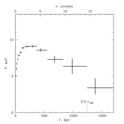
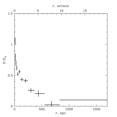
Figure 13.— Temperature and metallicity profiles for A2029.

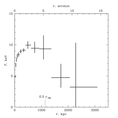
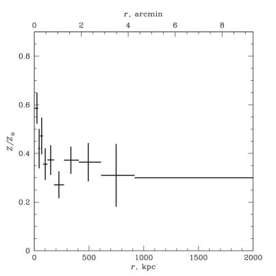
Figure 14.— Temperature and metallicity profiles for A2390.

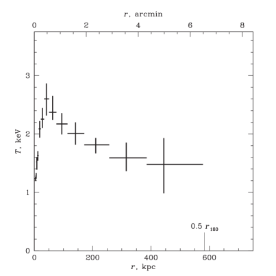
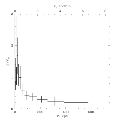
Figure 15.— Temperature and metallicity profiles for RXJ 1159+5531

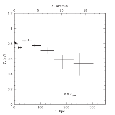
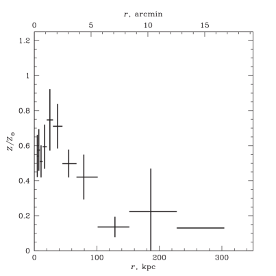
Figure 16.— Temperature and metallicity profiles for USGC S152

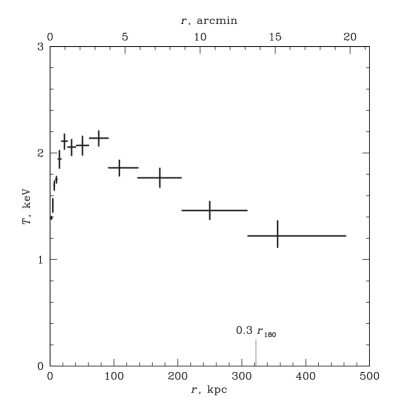
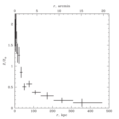
Figure 17.— Temperature and metallicity profiles for MKW4

3.10. Abell 2390

Abell 2390, the hottest and highest-redshift cluster in our sample ($z=0.2304$) was observed in 3 ACIS-S pointings for 10, 10, and 100 ksec. We discard the first two short observations. One of them was performed in 1999 and accurate gain calibration for this period is unavailable. The second short observation was telemetered in FAINT mode, which results is poorer background rejection. The X-ray image shows some substructure in the central $1.6^{\prime}$ or $\sim 300$ kpc (cavities and elongations) but is more regular on larger scales (Fig. 1). The best-fit absorption is constant with radius, $N_{H}=(1.07\pm 0.05)\times 10^{21}$ cm^-2, but is higher than the radio value $6.8\times 10^{20}$ cm^-2; we use the X-ray value in the further analysis. The spectra from the outermost regions show positive soft-band residuals which can be fit with the MEKAL spectrum with $T=0.24$ keV and normalization corresponding to the 0.7–2 keV flux $(8.9\pm 2.7)\times 10^{-6}$ cnt s^-1 arcmin^-2; this was used as an additional soft background correction. The temperature and metallicity profiles are shown in Fig. 14. There is a marginally significant temperature drop from $T\simeq 9.5$ keV at $r\sim 500$ kpc to $4.7\pm 2.3$ keV at $r>1200$ kpc.

3.11. RXJ 1159+5531

RXJ 1159+5531 ($T=1.9$ keV, $z=0.081$) is an “X-ray Over-Luminous Elliptical Galaxy” selected from the 160 deg² ROSAT PSPC Survey (Vikhlinin et al., 1999). Optically, this object appears as a nearly isolated elliptical galaxy but its X-ray luminosity and extent is typical of poor clusters. It was observed in ACIS-I for 20 ksec in the Fall of 1999 and in ACIS-S for 80 ksec in 2004. Accurate calibration is still unavailable for the 1999 data and so we do not use this pointing in the present analysis. The optical structure suggests that this object is probably dynamically old and fully relaxed. The only detectable substructure in the X-ray image is, indeed, confined to the very central region of the cluster, $r<5$ kpc. The average X-ray absorption is consistent with the radio column density, $N_{H}=1.2\times 10^{20}$ cm^-2. The soft background is clearly over-subtracted. The required correction is well-fit by a MEKAL spectrum with $T=0.17$ keV and negative normalization similar to most of other similar cases. The temperature and metallicity profiles of RXJ 1159+5531 are shown in Fig. 15.

3.12. USGC S152

The next two clusters are low-redshift, low-temperature systems. USGC S152 ($z=0.0153$) was observed in a single ACIS-S pointing for 30 ksec (Fig. 1). This is the lowest-temperature ($T\sim 0.8$ keV) cluster in our sample. The outermost region of the field of view ($r>16.5^{\prime}$) is virtually free from the cluster emission and the spectrum extracted at these radii shows no problems with the background subtraction in the soft band. The best-fit absorption is $N_{H}=(1.55\pm 0.10)\times 10^{21}$ cm^-2, which is significantly higher than the radio value, $4.34\times 10^{20}$ cm^-2; there are no statistically significant variations of absorption with radius. The temperature and metallicity profiles are shown in Fig. 16. This is the only cluster in our sample without a strong central temperature decrement, probably because the energy output from a recent AGN outburst or from the stellar winds of the central cD galaxy is non-negligible in this low-temperature system.

3.13. MKW4

MKW4 ($z=0.0199$) was observed in a single ACIS-S pointing for 30 ksec (Fig. 1). Faint cluster emission is detectable to the very edge of the ACIS field of view. We find no indication of problems with the soft background subtraction. However, the best-fit absorption is significantly higher than the radio value ($1.89\times 10^{20}$ cm^-2) and varies with radius from $(6.4\pm 0.8)\times 10^{20}$ cm^-2 near the cluster center to $(2.6\pm 0.8)\times 10^{20}$ cm^-2 in the outermost regions. We, therefore, allowed $N_{H}$ to be a free parameter in the spectral fits. The results for this cluster are shown in Fig. 17. Note a remarkably strong metallicity gradient — $Z$ changes (for a single-temperature model) from $\sim 2$ Solar in the center to $<0.3$ Solar outside the central 200 kpc.

4. Discussion of systematic effects

To the best of our knowledge, all calibration effects which could affect the temperature profile measurements have been accounted for in our analysis. It is useful, nevertheless, to discuss independent indicators of systematic errors. The main possible sources of bias are the following. (i) Statistical. Our spectral fits use $\chi^{2}$ minimization. The cluster emission is fainter at large radii and the photon counting statistics are increasingly non-Gaussian, which in principle can lead to underestimation of the temperature. The statistical bias can be avoided by adequately grouping the spectra, so that there is a sufficient number of counts in each bin prior to background subtraction. The binning we used — into 26 channels of approximately equal log width — resulted in $>100$ counts per channel in all cases. Therefore, $\chi^{2}$ statistics are fully adequate for spectral fitting; this was verified in several cases by fitting the spectra with a factor of 2 coarser binning.

(ii) Effective area. Miscalibration of the off-axis effective area can result in artificial temperature gradients. However, effective area calibration can be verified internally from our data. The most sensitive test is provided by different pointings of A1795, with the cluster placed at different detector locations and off-axis angles in both ACIS-S and ACIS-I. If miscalibration of effective area were responsible for an observed factor of $\sim 2$ temperature decrease at large radii we would derive very different temperatures for the central region of A1795 from on-axis and off-axis pointings. Instead, we find excellent agreement between these pointings (see §3.3 and full report in Vikhlinin et al. 2004a). Further evidence against effective area-related bias is provided by the off-axis ACIS-I observation of A133 which resulted in one of our most accurate temperature profiles (Fig. 3). Unlike most other cases, the cluster center in this pointing was placed off-axis and the temperature decrease is observed on-axis. Finally, miscalibration of effective area would tend to cause all temperature profiles to be similar when plotted as a function of angular distance from the center. Instead, we observe a very large scatter in such a plot (Fig. 18a).

(iii) Background. Incorrect background subtraction can affect temperature measurements at large radii where the surface brightness is low. If incorrect background subtraction is the cause for temperature decrements at large radii, the background normalization must be overestimated in all cases we analyzed. This is unlikely given that we used a procedure that was demonstrated to work very well for a large number of Chandra observations (Markevitch et al. 2003). Typical scatter of the background normalization is included in our temperature uncertainties. The accuracy of the background subtraction can be verified directly for several clusters with small angular size that we observed in ACIS-I, such as A383 and A907, because a sufficient fraction of the ACIS field of view is free from cluster emission in these cases. There are no background residuals in these areas, and the temperature profiles for these two clusters are typical of the entire sample.

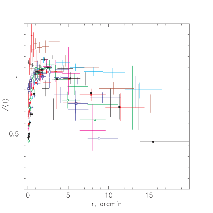
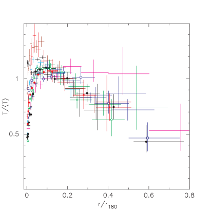
Figure 18.— Temperature profiles for all clusters plotted as a function of angular distance from the center and in units of the cluster virial radius. The temperatures were scaled to the cluster emission-weighted temperature excluding the central 70 kpc regions affected by cooling. The virial radii were estimated from these average temperatures using a relation from Evrard et al. (1996), $r_{180}=2.74\,\text{Mpc}\;(\langle T\rangle/10\,\text{keV})^{1/2}$. Our best measurements, for A1991 ($T=2.6$ keV), A133 ($T=4.2$ keV), A1413 ($T=7.3$ keV), and A2029 ($T=8.5$ keV), are open circles, filled circles, open squares, and filled squares, respectively. The strongest outliers in the right panel are MKW 4 (brown) and RXJ 1159+5531 (red) whose temperature profile peak at $r<70$ kpc, and A2390 (magenta) whose central cool region extends to $r\sim 400$ kpc.

To summarize, we cannot identify any obvious source of systematic error which could be responsible for the observed temperature decrease at large radii. An implicit indication that our measurements are correct is given by the similarity of all temperature profiles when expressed in units of the virial radius, as discussed below.

5. Self-similarity of temperature profiles

Theory predicts that clusters should be approximately self-similar because they form from scale-free density perturbations, and their dynamics are governed by the scale-free gravitational force. Self-similarity implies, in particular, that cluster temperature (and density etc.) profiles should be similar when radii are scaled to the cluster virial radius, which can be estimated from the average temperature, $r_{180}\propto\langle T\rangle^{1/2}$ (for detailed discussion see, e.g., Bryan & Norman 1998). This prediction is strongly confirmed by our measurements.

The scaled temperature profiles for all clusters are shown in Fig. 18b. The temperatures were scaled to the integrated emission-weighted temperature, excluding the central $70$ kpc region usually affected by radiative cooling. The same average temperature was used to estimate the cluster virial radius, $r_{180}$ using a relation from Evrard, Metzler & Navarro (1996), $r_{180}=1.95\,h^{-1}\,\text{Mpc}(\langle T\rangle/10\,\text{keV})^{1/2}$. The scaled profiles are almost identical at $r\gtrsim 0.15r_{180}$ and the general trend can be represented with the following functional form,

$$T/\langle T\rangle=\begin{cases}1.07,&\text{$0.035<r/r_{180}<0.125$}\\ 1.22-1.2\,r/r_{180},&\text{$0.125<r/r_{180}<0.6$},\end{cases}$$ (2)

with a 15–20% scatter. The only significant outlier is A2390 (shown in magenta). However, this cluster is unusual in that its central cool region in this cluster extends to $r\sim 400$ kpc, probably because the cold gas is pushed out from the center by radio lobes.

The strongest scatter of the temperature profiles is observed in the central cooling regions. This is not unexpected, because in these regions, non-gravitational processes such as radiative cooling and energy output from the central AGNs are important, thus breaking self-similarity. The largest outliers in the central region are MKW 4 and RXJ 1159+5531 whose cooling regions are very compact and the temperature profiles peak near $r\simeq 50$ kpc (thus our fixed exclusion radius of 70 kpc is too big).

Some of the previous studies of large cluster samples with ASCA and Beppo-SAX have already uncovered the similarity of the cluster temperature profiles at large radii (Markevitch et al., 1998; De Grandi & Molendi, 2002). Our measurements are consistent with these earlier results both qualitatively and quantitatively. Red band in Fig. 19 represents the typical scatter of individual profiles in the M98 sample. Our radial trend at $r>0.1\,r_{180}$ is in good agreement with their profile, even though our sample has only two clusters in common with M98 (A478 and A1795). A difference in the qualitative trend around $0.1\,r_{180}$ is fully expected, considering that the ASCA measurement was at the limit of that instrument’s angular resolution, and given the difference in spectral modeling (we use single-temperature fits whereas M98 used a then-common model with ambient + cooling flow components for the cluster centers, and included only the ambient hot phase in the final profiles).

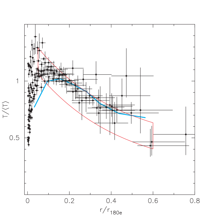
Figure 19.— Comparison of the Chandra temperature profiles and the average profiles from ASCA (Markevitch et al., 1998) and Beppo-SAX (De Grandi & Molendi, 2002). ASCA results are shown as the red band with the width equal to the scatter of the best-fit values in a sample of 30 clusters. Beppo-SAX results (blue line) represent the average temperature profile in a sample of 11 “cooling flow” clusters.

The average Beppo-SAX profile for the subsample of clusters with cool cores (such as ours) from De Grandi & Molendi (2002) is shown by blue line in Fig. 19. The results are remarkably close at $r>0.2\,r_{180}$. At smaller radii, the Beppo-SAX profile does not recover the continuation of a temperature increase towards smaller radii, which is consistent with the poorer angular resolution of that telescope.

A declining temperature profile has been recently reported from an XMM analysis of 16 low-redshift clusters (Piffaretti et al., 2004). On average, temperature drops by $\sim 30\%$ from its peak value near $r=0.4r_{180}$ (the outer radius for most clusters in Piffaretti et al. sample), fully consistent with our results.

Declining temperature profiles are generally reproduced in recent cosmological numerical simulations (Loken et al., 2002; Ascasibar et al., 2003; Valdarnini, 2003; Borgani et al., 2004; Ettori et al., 2004; Kay et al., 2004; Motl et al., 2004), although earlier simulations were more discrepant and produced both nearly isothermal profiles (Evrard et al., 1996) and strong temperature gradients (Katz & White, 1993). The best agreement with observed temperature profile seems to be reached by Eulerian codes (Loken et al. 2002 and discussion therein) and by the entropy-conserving versions of the SPH code (Springel & Hernquist, 2002) used, e.g., by Ascasibar et al. and Borgani et al. A more detailed comparison with observations requires folding the simulation output through the detector response (Mazzotta et al., 2004). This is beyond the scope of this paper. The general agreement of numerical and observational results suggests that the declining temperature profiles is a natural product of gravitational heating of ICM in the process of cluster formation. This conclusion is unaffected by the presence of heat conductivity of up to 1/3 of Spitzer value (Dolag et al., 2004).

6. Summary and conclusions

Chandra is well-suited for measurements of the temperature profiles to 0.5–0.6 of the virial radius thanks to its stable detector background, and fine angular resolution. Our analysis of high-quality observations of 11 low-redshift clusters reveals an almost universal behavior of temperature profiles in the systems spanning the range of average temperatures from 1 to 10 keV. Projected temperature as a function of radius reaches a maximum at $r\sim 0.1-0.2r_{180}$, just outside the central cooling region. The temperature gradually declines at larger radii, reaching 0.5 of its peak value near $r\sim 0.5-0.6r_{180}$, the outer boundary of our measurements in most cases.

In the future papers, we will use these Chandra observations for accurate measurements of the baryon and total mass profiles at large radii. We will also carry out a consistent comparison of clusters from high-resolution numerical simulations with their real-world counterparts.

References

- Ascasibar et al. (2003) Ascasibar, Y., Yepes, G., Müller, V., & Gottlöber, S. 2003, MNRAS, 346, 731
- Arnaud et al. (2001) Arnaud, M., Neumann, D. M., Aghanim, N., Gastaud, R., Majerowicz, S., & Hughes, J. P. 2001, A&A, 365, L80
- Belsole et al. (2004) Belsole, E., Pratt, G. W., Sauvageot, J.-L., & Bourdin, H. 2004, A&A, 415, 821
- Belsole et al. (2005) Belsole, E., Sauvageot, J., Pratt, G. W., & Bourdin, H. 2005, A&A, 430, 385
- Blanton et al. (2004) Blanton, E. L., Sarazin, C. L., McNamara, B. R., Clarke, T. E. 2004, ApJ, 612, 817.
- Borgani et al. (2004) Borgani, S., et al. 2004, MNRAS, 348, 1078
- Bryan & Norman (1998) Bryan, G. L. & Norman, M. L. 1998, ApJ, 495, 80
- Buote & Lewis (2004) Buote, D. A. & Lewis, A. D. 2004, ApJ, 604, 116
- Cannon, Ponman, & Hobbs (1999) Cannon, D. B., Ponman, T. J., & Hobbs, I. S. 1999, MNRAS, 302, 9
- Clarke et al. (2004) Clarke, T. E., Blanton, E. L., & Sarazin, C. L. 2004, ApJ, 616, 178
- David, Jones, & Forman (1996) David, L. P., Jones, C., & Forman, W. 1996, ApJ, 473, 692
- David et al. (2001) David, L. P., Nulsen, P. E. J., McNamara, B. R., Forman, W., Jones, C., Ponman, T., Robertson, B., & Wise, M. 2001, ApJ, 557, 546
- De Grandi & Molendi (2001) De Grandi, S. & Molendi, S. 2001, ApJ, 551, 153
- De Grandi & Molendi (2002) De Grandi, S. & Molendi, S. 2002, ApJ, 567, 163
- Dickey & Lockman (1990) Dickey, J. M. & Lockman, F. J. 1990, ARA&A, 28, 215
- Dolag et al. (2004) Dolag, K., Jubelgas, M., Springel, V., Borgani, S., & Rasia, E. 2004, ApJ, 606, L97
-
Edgar et al. (2004)
Edgar, R. J., et al. 2004,
Chandra calibration memo
(http://cxc.harvard.edu/cal/Acis/Cal_prods/qe/qe_memo.ps). - Ettori et al. (2000) Ettori, S., Bardelli, S., De Grandi, S., Molendi, S., Zamorani, G., & Zucca, E. 2000, MNRAS, 318, 239
- Ettori et al. (2004) Ettori, S., et al. 2004, MNRAS, 354, 111
- Evrard et al. (1996) Evrard, A. E., Metzler, C. A., & Navarro, J. F. 1996, ApJ, 469, 494
- Finoguenov, Arnaud, & David (2001) Finoguenov, A., Arnaud, M., & David, L. P. 2001, ApJ, 555, 191
- Fujita et al. (2002) Fujita, Y., Sarazin, C. L., Kempner, J. C., Rudnick, L., Slee, O. B., Roy, A. L., Andernach, H., & Ehle, M. 2002, ApJ, 575, 764
- Grant et al. (2004) Grant, C. E., Bautz, M. W., Kissel, S. M., & LaMarr, B. 2004, Proc. SPIE 5501 (astro-ph/0407199)
- Ikebe et al. (1997) Ikebe, Y., et al. 1997, ApJ, 481, 660
- Irwin & Bregman (2000) Irwin, J. A. & Bregman, J. N. 2000, ApJ, 538, 543
- Johnstone et al. (2002) Johnstone, R. M., Allen, S. W., Fabian, A. C., & Sanders, J. S. 2002, MNRAS, 336, 299
- Katz & White (1993) Katz, N. & White, S. D. M. 1993, ApJ, 412, 455
- Kay et al. (2004) Kay, S. T., Thomas, P. A., Jenkins, A., & Pearce, F. R. 2004, MNRAS, 504
- Lewis, Buote & Stocke (2003) Lewis, A. D., Buote, D. A., & Stocke, J. T. 2003, ApJ, 586, 135
- Loken et al. (2002) Loken, C., Norman, M. L., Nelson, E., Burns, J., Bryan, G. L., & Motl, P. 2002, ApJ, 579, 571
- Lumb, Warwick, Page, & De Luca (2002) Lumb, D. H., Warwick, R. S., Page, M., & De Luca, A. 2002, A&A, 389, 93
- Majerowicz, Neumann & Reiprich (2002) Majerowicz, S., Neumann, D. M., & Reiprich, T. H. 2002, A&A, 394, 77
- Markevitch et al. (1996) Markevitch, M., Mushotzky, R., Inoue, H., Yamashita, K., Furuzawa, A., & Tawara, Y. 1996, ApJ, 456, 437
- Markevitch et al. (1998) Markevitch, M., Forman, W. R., Sarazin, C. L., & Vikhlinin, A. 1998, ApJ, 503, 77
- Markevitch, Vikhlinin, Forman, & Sarazin (1999) Markevitch, M., Vikhlinin, A., Forman, W. R., & Sarazin, C. L. 1999, ApJ, 527, 545
- Markevitch et al. (2000a) Markevitch, M., et al. 2000, ApJ, 541, 542
- Markevitch et al. (2000b) Markevitch, M., Vikhlinin, A., Mazzotta, P., & Van Speybroeck, L. 2000b, in Proc. ”X-ray astronomy 2000” (Palermo, September 2000), Eds. R. Giacconi, L. Stella, S. Serio, ASP Conf. Series (astro-ph/0012215)
- Markevitch (2002) Markevitch, M. 2002, preprint, astro-ph/0205333
- Markevitch & Vikhlinin (2001) Markevitch, M. & Vikhlinin, A. 2001, ApJ, 563, 95
- Markevitch et al. (2003) Markevitch, M., et al. 2003, ApJ, 583, 70
-
Marshall et al. (2003)
Marshall, H. L., et
al. 2003, Chandra Calibration Workshop
(http://cxc.harvard.edu/ccw/proceedings/03_proc/presentations/marshall2). - Marshall et al. (2004) Marshall, H. L., Tennant, A., Grant, C. E., Hitchcock, A. P., O’Dell, S. L., & Plucinsky, P. P. 2004, Proc. SPIE, 5165, 497 (astro-ph/0308332)
- Mazzotta et al. (2002) Mazzotta, P., Kaastra, J. S., Paerels, F. B., Ferrigno, C., Colafrancesco, S., Mewe, R., & Forman, W. R. 2002, ApJ, 567, L37
- Mazzotta et al. (2004) Mazzotta, P., Rasia, E., Moscardini, L., & Tormen, G. 2004, MNRAS, 354, 10
- Motl et al. (2004) Motl, P. M., Burns, J. O., Normal, M. L., & Bryan, G. L. 2004, The Riddle of Cooling Flows in Galaxies and Clusters of galaxies,
- Nevalainen et al. (2001) Nevalainen, J., Kaastra, J., Parmar, A. N., Markevitch, M., Oosterbroek, T., Colafrancesco, S., & Mazzotta, P. 2001, A&A, 369, 459
- Nevalainen et al. (2004) Nevalainen, J., Markevitch, M., & Lumb, D. 2004, ApJ, submitted
- Peterson et al. (2001) Peterson, J. R., et al. 2001, A&A, 365, L104
- Piffaretti et al. (2004) Piffaretti, R., Jetzer, P., Kaastra, J., Tamura, T. 2004, A&A, in press (astro-ph/0412233)
- Pointecouteau et al. (2004) Pointecouteau, E., Arnaud, M., Kaastra, J., & de Plaa, J. 2004, A&A, 423, 33
- Pratt, Arnaud, Aghanim (2001) Pratt, G. W., Arnaud, M. & Aghanim, N. 2001, Clusters of Galaxies and the High Redshift Universe Observed in X-rays, ed. D.M. Neumann, & J. Trân Thanh Van (astro-ph/0105431)
- Pratt & Arnaud (2002) Pratt, G. W. & Arnaud, M. 2002, A&A, 394, 375
- Pratt & Arnaud (2004) Pratt, G. W. & Arnaud, M. 2004, A&A, in press (astro-ph/0406366)
- Sarazin (1988) Sarazin, C. L. 1988, X-ray Emission from Clusters of Galaxies (Cambridge: Cambridge University Press)
- Sakelliou & Ponman (2004) Sakelliou, I. & Ponman, T. J. 2004, MNRAS, 351, 1439
- Sanderson, Finoguenov & Mohr (2004) Sanderson, A. J. R., Finoguenov, A., & Mohr, J. J. 2004, ApJ, submitted (astro-ph/0412316)
- Sharma et al. (2004) Sharma, M., et al. 2004, ApJ, 613, 180
- Schmidt, Allen & Fabian (2001) Schmidt, R. W., Allen, S. W., & Fabian, A. C. 2001, MNRAS, 327, 1057
- Springel & Hernquist (2002) Springel, V. & Hernquist, L. 2002, MNRAS, 333, 649
- Sun et al. (2003a) Sun, M., Jones, C., Murray, S. S., Allen, S. W., Fabian, A. C., & Edge, A. C. 2003a, ApJ, 587, 619
- Sun et al. (2003b) Sun, M., Forman, W., Vikhlinin, A., Hornstrup, A., Jones, C., & Murray, S. S. 2003b, ApJ, 598, 250
- Takahashi & Yamashita (2003) Takahashi, S. & Yamashita, K. 2003, PASJ, 55, 1105
- Townsley et al. (2000) Townsley, L. K., Broos, P. S., Garmire, G. P., & Nousek, J. A. 2000, ApJ, 534, L139
- Valdarnini (2003) Valdarnini, R. 2003, MNRAS, 339, 1117
- Vikhlinin et al. (1999) Vikhlinin, A., McNamara, B. R., Hornstrup, A., Quintana, H., Forman, W., Jones, C., & Way, M. 1999, ApJ, 520, L1
-
Vikhlinin (2004a)
Vikhlinin, A. 2004a,
Chandra calibration memo
(http://cxc.harvard.edu/contrib/alexey/contmap.pdf). -
Vikhlinin (2004b)
— — — 2004b,
Chandra calibration memo
(http://cxc.harvard.edu/contrib/alexey/qeu.pdf). - Wargelin et al. (2004) Wargelin, B. J., Markevitch, M., Juda, M., Kharchenko, V., Edgar, R., & Dalgarno, A. 2004, ApJ, 607, 596
- Zhang et al. (2004) Zhang, Y.-Y., Finoguenov, A., Böhringer, H., Ikebe, Y., Matsushita, K., & Schuecker, P. 2004, A&A, 413, 49