An $850\mathrm{\mu m}$ SCUBA map of the Groth Strip and reliable source extraction

Abstract

We present an $850\,\mathrm{\mu m}$ map and list of candidate sources in a sub-area of the Groth Strip observed using SCUBA. The map consists of a long strip of adjoining jiggle-maps covering the southwestern $70\,\mathrm{arcmin^{2}}$ of the original WFPC2 Groth Strip to an average $1\,\sigma$ rms noise level of $\simeq 3.5\,\mathrm{mJy}$. We initially detect 7 candidate sources with signal-to-noise ratios (SNRs) between 3.0 and $3.5\,\sigma$ and 4 candidate sources with SNR $\geq 3.5$. Simulations suggest that on average in a map this size one expects 1.6 false positive sources $\geq 3.5\,\sigma$ and 4.5 between 3 and $3.5\,\sigma$. Flux boosting in maps is a well known effect and we have developed a simple Bayesian prescription for estimating the unboosted flux distribution and used this method to determine the best flux estimates of our sources. This method is easily adapted for any other modest signal-to-noise survey in which there is prior knowledge of the source counts. We performed follow-up photometry in an attempt to confirm or reject 5 of our source candidates. We failed to significantly re-detect 3 of the 5 sources in the noisiest regions of the map, suggesting that they are either spurious or have true fluxes close to the noise level. However, we did confirm the reality of 2 of the SCUBA sources, although at lower flux levels than suggested in the map. Not surprisingly, we find that the photometry results are consistent with and confirm the de-boosted map fluxes. Our final candidate source list contains 3 sources, including the 2 confirmed detections and 1 further candidate source with $\mathrm{SNR}>3.5\,\sigma$ which has a reasonable chance of being real. We performed correlations and found evidence of positive flux at the positions of XMM-Newton X-ray sources. The 95 per cent lower limit for the average flux density of these X-ray sources is $0.8\,\mathrm{mJy}$.

1 Introduction

Large blank-field SCUBA surveys have revolutionized our understanding of the importance and diverse nature of dusty galaxies at high redshifts (e.g. Blain et al. 2002, Scott et al. 2002, Webb et al. 2003, Borys et al. 2003). Only about 300 blank-field SCUBA galaxies have been discovered since the instrument was commissioned, in contrast to the tens of thousands to millions of objects detected in optical surveys of similar sizes. Nevertheless, the number counts have been well-characterised, and progress is being made in identifying SCUBA galaxies with objects in other wavebands using source positions derived from radio identifications.

However, the fact remains that SCUBA sources are difficult to find, and when they are detected they typically have low signal-to-noise ratios (SNRs), bringing into question the reliability of measurements. Using deep radio imaging of the 8-mJy Survey fields, Ivison et al. (2002) have suggested that low SNR sources in relatively noisy regions of submillimetre maps which lack radio counterparts are often spurious. Additional evidence that these sources might be spurious comes from the lack of MAMBO (Max Planck Millimeter Bolometer array) counterparts to many of these SCUBA sources (Greve et al. 2004). Mortier et al. (2004) also report not recovering a similar fraction of low SNR sources in the 8-mJy Survey region when combined with newer SHADES (SCUBA HAlf Degree Extragalactic Survey) data in the same field. Only one region, namely the Hubble Deep Field (HDF) region or GOODS-North field, has been investigated independently by different groups. Reassuringly, Borys et al. (2003, 2004) and Wang, Cowie & Barger (2004) are in close agreement for the higher SNR sources in that region. However, there is some disagreement regarding the reality and the flux densities of several of the noisier sources. The effects of flux boosting (sometimes called Malmquist and/or Eddington bias) are well known for SNR-thresholded maps, and it is worthwhile to investigate whether such discrepancies are to be expected, and when one should be confident about the reality of a source, independent of whether it has a radio identification. It is clear that a careful, un-biased analysis of the robustness of SCUBA detections in shallow maps is called for. In this vein we provide a careful estimate of flux boosting and have followed up in photometry mode 5 sources detected in a shallow $850\,\mathrm{\mu m}$ map of the Groth Strip, in an attempt to quantify the amount of flux boosting present in the map. To interpret the results we have developed a general method to assess the reliability of low SNR sources.

We apply these techniques to a particular SCUBA survey in the ‘Groth Strip’. The ‘Groth Strip Survey’ (GSS) is a Hubble Space Telescope (HST) programme (GTO 5090, PI: Groth) consisting of 28 overlapping HST Wide Field Planetary Camera 2 (WFPC2) medium-deep images, covering an area of $113\,\mathrm{arcmin^{2}}$, forming a long strip centred on RA=$14^{\mathrm{h}}16^{\mathrm{m}}38{\aas@@fstack{s}}8$, Dec=$52^{\circ}16^{\prime}52^{\prime\prime}$ (J2000), at a Galactic latitude of $b\simeq 60^{\circ}$. The GSS was the deepest HST cosmological integration before the HDF, reaching a limiting Vega magnitude of $\sim 27.5$–28 in both the V and I bands (Groth et al., 1994). The GSS has an enormous legacy value, since extensive multi-wavelength observations centred on this region have been conducted or are planned. Morphological and photometric information from the WFPC2 images are provided by the Medium Deep Survey (MDS) database (Ratnatunga, Griffiths & Ostrander, 1999) and the Deep Extragalactic Evolutionary Probe (DEEP) survey (Simard et al., 2002). X-ray sources have also been identified in an $80\,\mathrm{ks}$ XMM-Newton observation of the GSS (Miyaji et al., 2004). The GSS is currently part of the on-going DEEP2 survey and is also targetted to be a major component of upcoming large surveys in the UV (using the Galaxy Evolution Explorer, GALEX), in the optical (as part of the Canada-France-Hawaii Telescope Legacy Survey, CFHTLS), and in the IR (the Spitzer GTO IRAC Deep Survey).

In this paper, we present $850\,\mathrm{\mu m}$ SCUBA observations of about 60 per cent of the original WFPC2 coverage of the GSS. We have also performed confirmation photometry on some of the sources. Our goal is to make the $850\,\mathrm{\mu m}$ map and source list available to the community so that it may be correlated against existing and future data sets at other wavelengths. No claim is made that this survey is either the deepest or the most extensive performed using SCUBA. However, the observations cover enough integration time that we expect a handful of real sources to be detected, and our survey represents the best submillimetre data likely to be available in this field until the advent of SCUBA-2.

2 Map Observations and Data Reduction

A roughly $70\,\mathrm{arcmin}^{2}$ portion of the Groth Strip (GSS) was observed with a resolution of 14.7 arcsec and 7.5 arcsec at 850 and $450\,\mathrm{\mu m}$, respectively, with the 15-m JCMT atop Mauna Kea in Hawaii in January 1999 and January 2000. The GSS SCUBA map is centred on RA$\,{=}\,14^{\mathrm{h}}16^{\mathrm{m}}00^{\mathrm{s}}$, Dec$\,{=}\,52^{\circ}10^{\prime}00^{\prime\prime}$ (J2000).

52 overlapping 64-point jiggle maps of the GSS were obtained, providing measurements of the continuum at both wavelengths simultaneously with SCUBA (Holland et al., 1999), which has a field of view of 2.3 arcmin.

The atmospheric zenith opacity at $225\,\mathrm{GHz}$ was monitored with the Caltech Submillimetre Observatory (CSO) tau ($\tau_{\mathrm{CSO}}$) monitor. The $\tau_{\mathrm{CSO}}$ ranged from 0.03 to 0.09 in January 1999 and from 0.05 to 0.08 in January 2000. The weather was generally more stable for the latter set of data.

The secondary mirror was chopped at a standard frequency of $\simeq 8\,\mathrm{Hz}$ in azimuth to reduce the effect of rapid sky variations. The telescope was also ‘nodded’ on and off the source. A 40 arcsec chop–throw was used at a position angle of $54^{\circ}$, almost parallel to the lengthwise orientation of the strip. Pointing checks were performed hourly on blazars and planets and varied by less than 3 arcsec in azimuth and by less than 2 arcsec in elevation. The overlapping jiggle maps were co-added to produce a final map with a total integration time of 18 hours and 50 minutes.

We used SURF (SCUBA User Reduction Facility; Jenness & Lightfoot 1998) scripts together with locally developed code (Borys, 2002) to reduce the data. The SURF map and our map look similar. The benefit of using our own code to analyse the data is that it makes a map with minimally correlated pixels and provides an estimate of the noise in each pixel. We chose 3 arcsec pixels oriented along RA,Dec coordinates. This pixel size is slightly too large for $450\,\mathrm{\mu m}$ studies, but has proven to be adequate at $850\,\mathrm{\mu m}$ (see Borys et al. 2003).

2.1 Flux Calibration

Calibration data were reduced in the same way as the GSS data. The flux conversion factors (FCFs) over 3 of the 4 nights in January 1999 and all 3 nights in January 2000 agree with the monthly averages to within 10 per cent (see the JCMT calibration web-page). The FCF value for one night in January was 30 per cent higher than the monthly average and this could indicate that the sky was so variable that the $\tau_{\rm CSO}$ was not accurately reflecting the opacity along the line of sight to the object. The calibration uncertainty is omitted from our quoted error values since it is not a major contributor to the global uncertainty of our low SNR data and has no effect on our source detection method.

The $850\,\mathrm{\mu m}$ map has a mean consistent with zero, as expected from differential measurements, and an rms of $3.5\,\mathrm{mJy}$. The final map is shown in Fig. 1. The $450\,\mathrm{\mu m}$ map also has a mean consistent with zero and an rms of $50\,\mathrm{mJy}$.

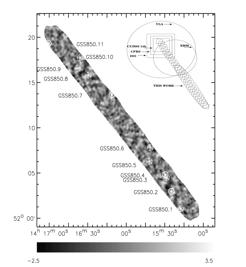
Figure 1: The $850\,\mathrm{\mu m}$ SNR image of the Groth Strip, smoothed with the 3-beam template (see $\S~{}\,\ref{sourcedet}$). The solid 40-arcsec diameter circles correspond to candidate sources with $\mathrm{SNR}\geq 3.5$. Dashed circles indicate the positions of the SNR$\,{=}\,3.0$–3.5 candidate sources. The inlay in the top right-hand corner illustrates our field geometry relative to some other surveys in this region, including the original WFPC pointings (jagged squares), the CUDSS+14 field, CFRS and ISO survey regions (trio of large squares, listed here in order of increasing size), VLA coverage (large circle) and XMM coverage (smaller circle).

2.2 Source Detection Method

Given the 14.7 arcsec beam, a high-redshift galaxy will be unresolved and will appear as a positive source flanked by 2 negative sources. The source density at $850\,\mathrm{\mu m}$ (see e.g. Scott et al. 2002, Borys et al. 2003, Webb et al. 2003) suggests that only a handful of sources will be recovered in our map. Hence we do not expect many overlapping sources, and therefore sources were extracted by fitting the raw rebinned map with a three-lobed PSF of an isolated point-source with the same chop throw and position angle as the map data. A fit to the PSF model centred on each pixel is equivalent to a noise-weighted convolution and is the minimum variance estimator if the background consists of white noise. An accompanying weighted noise map is created simultaneously and provides an estimate of the noise associated with the detection of a point source in each pixel. A peak in the PSF-convolved map which is 3 times the noise in that pixel constitutes a $3\,\sigma$ detected point source.

3 Source Robustness

For a list of sources found above a given significance level in a map to be useful, one must address the following questions: ‘Are there any statistical anomalies in the data which would cause one to doubt any of the sources?’; ‘Given our actual noise and measurement strategy, what fraction of sources present at any given flux level would we expect to detect?’, that is, ‘How complete is our source list?’; and finally, ‘Do the fluxes inferred from the maps form a biased estimator of actual source flux?’ Bias and flux boosting are addressed in $\S~{}\ref{section4}$. Quality of fit and completeness are addressed here.

We investigate source robustness using several techniques, including spatial and temporal $\chi^{2}$ tests, searching for negative sources, and Monte Carlo simulations.

3.1 Spatial and Temporal $\chi^{2}$ Tests

Although a candidate source may be ‘detected’ in the map, it may not necessarily be well-fit by the PSF, or it may be a poor fit to the set of difference data, or both. We have performed spatial and temporal $\chi^{2}$ tests in order to determine how well the raw timestream data fit the final PSF-fitted maps. See Pope et al. (2004) for details.

The spatial $\chi^{2}$ test provides a gauge across the map of the goodness-of-fit of the triple-beam differential PSF to the data, and thus indicates if a source is poorly fit by the assumed PSF. We find that the $\chi^{2}$ values for each pixel where a source is detected are within $\pm 2\,\sigma$ (=$2\sqrt{2N_{\mathrm{pix}}}$), where $N_{\mathrm{pix}}$ is the of number degrees of freedom or number of pixels included in the fit) in all cases, except for GSS850.3, a candidate source with SNR=3.3. The poor fit may be the result of its proximity to GSS850.4 (see Fig. 1).

The temporal $\chi^{2}$ provides a measure of the self-consistency of the raw timestream data which contribute flux to each map pixel. For example, a portion of the hits on a pixel might be consistent with a certain flux value, whereas the rest of the hits might be most consistent with a different value. Following the prescription of Pope et al. (2004), we calculate the pixel temporal $\chi^{2}_{i}$ and the number of hits for each pixel $N_{\mathrm{hits}}^{i}$. We then essentially construct a SNR map of poorness-of-fit to the model by using the quantity $\chi^{2}_{i}-N_{\mathrm{hits}}^{i}$ as the ‘signal’ and $\sqrt{2N_{\mathrm{hits}}^{i}}$ as the ‘noise’ and fitting the PSF to this temporal $\chi^{2}$ map. We find that none of the pixels at the centres of our candidate sources lie outside the $\pm 2\,\sigma$ regions of our distribution. We are therefore confident that all of our candidate sources lie in regions of the map with self-consistent timestream data and have no grounds to reject any of our detected candidate sources based on these tests.

Note that these two tests also check for Gaussianity of the noise in the map, but they are not a strong test of this distribution.

3.2 Sources Detected in the Inverted Map

A quick test of source reality is to create the negative of the map and to search for sources using the same triple-beam template. Aside from pixels associated with the off-beams of positive detections, we find 6 ‘detections’ in the inverted map, consistent with the expected number of false positive detections in noisy data (see $\S~{}\ref{sims}$).

3.3 Monte Carlo Simulations

Simulations are required in order to evaluate map completeness and the likely rate of false positive detections, given our non-uniform noise. We follow the procedures described in Borys et al. (2003) for investigating the number of positive sources expected at random, as well as the map completeness.

In order to determine how many detections may be spurious, we created a map with the same shape and size as the real one, but replaced the $850\,\mathrm{\mu m}$ data with Gaussian random noise, generated using the rms of the timestream of each file and each bolometer. We then performed the same source detection procedure that was used on the real data. We repeated this sequence of steps 1000 times and plot the cumulative number of positive sources detected on average in Fig. 2 at each SNR threshold. The simulations suggest that on average one expects 1.6 false positive sources $>3.5\,\sigma$ and a further 4.5 between 3 and $3.5\,\sigma$.

Figure 2: Cumulative number of detected candidate sources. We plot results against SNR threshold for our map (dark histogram), the average expected in source-free simulated $850\,\mathrm{\mu m}$ maps containing only Gaussian random noise (light dotted curve), the number of false positives expected on average plus the predicted number of real sources using the source counts of Borys et al. (2003) multiplied by the completeness estimate (dark solid curve), and the confirmed spurious detections (light histogram, see $\S~{}\ref{section4}$). The number of expected detections and the number of actual detections are consistent within the Poisson noise.

The completeness of a map is the fraction of sources which one expects to detect at each flux level. To measure this fraction, we added a source of known flux into the real map and tried to extract it using our source extraction method. We selected the input source flux randomly in the range 3–$20\,\mathrm{mJy}$, located it uniformly across the map, and repeated this procedure 1000 times. A source is considered recovered if it is detected with $\mathrm{SNR}\geq 3$ and located within 7.5 arcsec (the $850\,\mathrm{\mu m}$ beam HWHM) of the input position. We estimate that about 60 per cent of the $>10\,\mathrm{mJy}$ sources are detected above a SNR of $3\,\sigma$ in the map (see Fig. 3). The completeness is slightly higher than it would be in a map with uniform noise at the same rms, as expected.

Figure 3: Completeness of $850\,\mu$m source recovery at each level of input flux for $3\,\sigma$ detections, as determined from the Monte Carlo simulations of individual sources added to the GSS data described in $\S~{}\,\ref{sims}$.

4 Candidate Submillimetre Sources

We detect 4 candidate sources with $\mathrm{SNR}\geq 3.5\,\sigma$ and 7 candidate sources with SNRs in the range 3.0–$3.5\,\sigma$. A submillimetre image of the GSS is shown in Fig. 1, where we number each of these 11 candidates, while in Table 1 we present information on the 5 sources for which we performed follow-up photometry (see $\S~{}\ref{phot}$). The signal and noise maps may be downloaded from http://cmbr.physics.ubc.ca/groth.

Table 1: GSS $850\,\mathrm{\mu m}$ candidate submillimetre sources with follow-up photometry. Locations of these and the other 6 candidate SCUBA sources are indicated in Fig 1.

Object	$S_{850}$	$S_{850}$
	(mJy)	(mJy)
GSS850.1	$9.5\pm 2.9\,(3.3\,\sigma)$	$-1.8\pm 3.6\,(-0.5\,\sigma)$
GSS850.2	$8.2\pm 2.3\,(3.6\,\sigma)$	$5.7\pm 1.1\,(5.2\,\sigma)$
GSS850.6	$12.3\pm 4.1\,(3.0\,\sigma)$	$1.2\pm 3.1\,(0.4\,\sigma)$
GSS850.7	$13.2\pm 3.2\,(4.1\,\sigma)$	$4.2\pm 1.7\,(2.5\,\sigma)$
GSS850.11	$11.2\pm 2.9\,(3.8\,\sigma)$	$0.1\pm 1.6\,(0.1\,\sigma)$

4.1 Additional Photometry

In December 2003 and January 2004, SCUBA photometry observations were performed in the 2-bolometer chopping mode to check some of our candidate map detections. We selected 2 candidates, GSS850.7 and GSS850.11, near the noisier edge regions of the map and a ‘control’, GSS850.2, in a lower-noise region away from the edges. Also, during one of the observing runs in January 2000, four sources were identified in the map data ‘by eye’ and selected as targets for follow-up photometry. Only two of these pointings correspond to candidate detections in the final map (GSS850.1 and GSS850.6); this is a warning that our eyes often pick out bright outliers in noisy regions of a map. All of the photometry observations were reduced in the standard way using SURF. In order to increase the SNR of sources observed in the 2-bolometer mode by a factor of approximately $\sqrt{3/2}$, we folded in the signal from the off-position bolometers to the central bolometer (see Chapman et al. 2000). The results are listed in Table 1 for comparison with the estimated map fluxes. In all cases, the photometry pointings were within 3 arcsec of the positions found by the source-detection algorithm in the map.

4.2 Flux Boosting in the Map

It appears that we have detected some sources in the map. However none of the candidate sources have very high SNRs, and so we need to be careful in interpreting these results. Confusion can either increase or decrease the input flux of a source, but a noisy flux-limited map will preferentially contain sources whose true fluxes have been increased (usually called Malmquist bias) and this effect is exacerbated for steep source counts. Our source extraction procedure therefore biases fluxes in the map upwards, which we now attempt to quantify.

Figure 4: The first panel shows the histogram of the 1 million noiseless triple-beam simulations described in $\S~{}\ref{boost}$. This is the $P(D)$ distribution (e.g. Scheuer 1974, Condon 1974) for a triple-beam experiment, which is strongly peaked around zero and skew positive due to sources. The other panels show the resulting flux probability distributions (dark histograms) for the 5 map source candidates which had follow-up photometry observations, given their measured fluxes and errors (assumed to be Gaussian distributions, plotted separately as light dot-dashed lines) and the underlying source count model. Photometry measurements are overplotted for comparison and are also assumed to have Gaussian probability distributions (dark dashed lines). A vertical line at $S_{\mathrm{p}}$=0 is plotted as a reference with which to compare the photometry measurements. One can see that the combination of the intrinsic distribution of fluxes and the low SNR measurements from the map make the photometry measurements much less inconsistent than they might appear (i.e. the dashed Gaussians compare well with the solid histograms, even although the two Gaussians in each panel are usually discrepant).

We performed a set of simulations to assess the expected distribution of pixel brightnesses from triple-beam (i.e. double difference) observations of a noiseless blank-sky. We used a smooth curve fit to (and mildly extrapolated from) the number counts of Borys et al. (2003) as an a priori distribution of fluxes in the range 0.1–$40\,\mathrm{mJy}$. We then populated 3 different patches of noiseless sky following a Poisson distribution, and sampled each area with a SCUBA Gaussian beam, taking a double difference each time. This was done 1 million times and the anticipated prior distribution of double difference flux measurements, $N(S_{\mathrm{p}})$, is plotted in the first panel of Fig. 4. We have also investigated the effects of reasonable excursions from the assumed shape of the source counts. For example, using the $1\,\sigma$ error bar values at the bright end of the number counts has less than a 10 per cent effect on the resulting flux estimates.

The distribution $N(S_{\mathrm{p}})$, which is the prior probability that a pixel in the map has differential flux $S_{\mathrm{p}}$, is calculated from noiseless simulations while our actual map contains noise. If $M$ is the statement that we measure flux $S_{\mathrm{m}}\pm\,\sigma_{\mathrm{m}}$ at some pixel in the map, the probability that the true flux of that pixel is $S_{\mathrm{p}}$ is obtained from Bayes’ theorem:

$$P(S_{\mathrm{p}})\equiv P(S_{\mathrm{p}}|M,N(S_{\mathrm{p}}))=\frac{N(S_{\mathrm{p}})\times P(M|S_{\mathrm{p}})}{P(M)},$$ (1)

where the probability we would measure $S_{\mathrm{m}}$ when the true flux is $S_{\mathrm{p}}$ is

$$P(M|S_{\mathrm{p}})=A\,e^{\frac{(S_{\mathrm{m}}-S_{\mathrm{p}})^{2}}{2\,\sigma_{\mathrm{m}}^{2}}},$$ (2)

under the assumption that our noise is Gaussian distributed. We have weakly tested this assumption in $\S~{}\ref{chi}$ $\mathrm{and}~{}\ref{invert}$. $P(M)$ acts as an overall normalisation in equation (1), and does not depend upon $S_{\mathrm{p}}$ as long as the noise is not correlated with sources on the sky. Strictly speaking, $P(M|S_{\mathrm{p}})$ should be altered from the form we have used to account for the fact that we are examining the probability at a location where we have found a peak. In practice, at $S_{\mathrm{m}}-S_{\mathrm{p}}\geq 3\,\sigma$ the full expression converges to the simpler form we have used (Bond & Efstathiou 1987).

The posterior flux probability distribution, $P(S_{\mathrm{p}})$ is shown as a solid histogram in the panels of Fig. 4 for each of the 5 sources for which we also have follow-up photometry information. The dot-dashed Gaussian in each panel is $P(M|S_{\mathrm{p}})$, which is often incorrectly adopted as the flux estimate of a map source.

In Fig. 4 we have placed the individual $P(S_{\mathrm{p}})$ plots in order of increasing map SNR. It is clear that one expects to measure a non-zero flux value a significant fraction of the time only for sources with relatively high SNRs. Sources with modest SNRs are much more likely to have non-zero photometry results than lower SNR sources. The peak in the a posteriori distribution at zero flux dominates for SNR $\lesssim 3.5$. This confirms the usual prejudice towards high SNR sources – if a source is bright, it needs to be detected with a $\mathrm{SNR}\gtrsim 4\,\sigma$ in order to be deemed a secure detection. Moreover, we also find that at the same SNR level, apparently brighter sources (with consequently higher flux uncertainty) are more likely to be spurious (i.e. flux boosted from $\simeq 0\,\mathrm{mJy}$) than fainter sources. Thus at a given SNR, low flux sources are more likely to be real than high flux sources.

We performed independent photometry observations on 5 sources with SNRs ranging from 3.0–$4.1\,\sigma$ and the results are shown in Table 1. We wish to know if the photometry measurements are consistent with the map-detected fluxes. In other words, we want to answer the question: ‘What is the probability that we will measure $S_{\mathrm{p}}$ in photometry mode given the map-detected flux ($S_{\mathrm{m}}$) and uncertainty ($\sigma_{\mathrm{m}}$) and the underlying source count model?’. The main point is that the a posteriori probability of finding a bright source will be down-weighted by the a priori probability coming from the source counts.

A comparison of the dashed curves and solid histograms in Fig. 4 shows that our photometry results are consistent with $P(S_{\mathrm{p}})$, even though the photometry is often inconsistent with the raw (i.e. flux boosted) map readings $P(M|S_{\mathrm{p}})$.

4.3 A Revised Source List

We can now assess the probability of obtaining each of the photometry measurements using the distributions in Fig. 4. For GSS850.6, a photometry result lower than what we measured is expected 43 per cent of the time. For the remaining sources GSS850.1, GSS850.2, GSS850.11 and GSS850.7, we have assessed that a photometry measurement lower than the one we obtained would have occurred 12, 60, 6, and 18 per cent of the time, respectively. A Kolmogorov-Smirnov (KS) test performed on these results determined that the set of 5 trials is consistent with a uniform distribution.

The photometry results are thus completely within the realm of what is expected, despite the apparently contradictory results presented in Table 1. We confirm GSS850.2 and GSS850.7 as bona fide $850\,\mathrm{\mu m}$ sources, and we confidently eliminate GSS850.1, GSS850.6, and GSS850.11 from our candidate source list. Note that these eliminated sources are also among the 4 noisiest candidate detections in the map, which makes it even less surprising that they are spurious. We have tallied up the number of detections, expected sources, and spurious detections and have illustrated these in Fig. 2. We note that the number counts (e.g. Scott et al. 2002, Borys et al. 2003, Webb et al. 2003) predict the detection of around 3 sources at the flux limit of the map ($\sim 10\,\mathrm{mJy}$).

Table 2: GSS $850\,\mathrm{\mu m}$ revised source list. We have included the 2 photometry-confirmed sources and an additional $>3.5$ candidate source which has a reasonable chance of being real. The best $850\,\mathrm{\mu m}$ flux estimate is given based on the combination of the posterior probability of the map flux given the data together with the photometry flux for the sources with photometry (2 and 7), and based solely on the posterior probability of the map flux for GSS850.4. The reported flux is the most likely flux in the 68 per cent confidence region, with upper and lower error bars shown to indicate the range of that confidence interval. 95 per cent Bayesian upper limits are also given for the $450\,\mathrm{\mu m}$ flux of each $850\,\mathrm{\mu m}$ detection.

Object	Position (2000.0)		$S_{850}$	$S_{450}$
	RA	Dec	(mJy)	(mJy)
GSS850.2	$14^{\mathrm{h}}15^{\mathrm{m}}25{\mathrm{\aas@@fstack{s}}}0$	$+52^{\circ}02^{\prime}57^{\prime\prime}$	$5.9^{+0.7}_{-1.2}$	$<170$
GSS850.4	$14^{\mathrm{h}}15^{\mathrm{m}}29{\mathrm{\aas@@fstack{s}}}5$	$+52^{\circ}04^{\prime}48^{\prime\prime}$	$6.9^{+2.0}_{-4.7}$	$<48$
GSS850.7	$14^{\mathrm{h}}16^{\mathrm{m}}11{\mathrm{\aas@@fstack{s}}}6$	$+52^{\circ}13^{\prime}42^{\prime\prime}$	$4.8^{+1.5}_{-1.9}$	$<118$

Our revised source list now includes 2 confirmed sources (with coordinates given in Table 2) as well as 1 other candidate which is $>3.5\,\sigma$ in the map. Although not confirmed by photometry, Figs. 2 and 4 suggest that SNR $>3.5$ sources have a reasonable chance of being real. We are able to calculate a best estimate of the flux for each of these objects using the combination of all available information, including the map measurements, photometry measurements and the source count prior. To do this we multiply the measured (assumed Gaussian) photometry flux probability distribution, $P(S_{\mathrm{p}},\sigma_{\mathrm{p}})$, by the calculated posterior probability for the map flux (equation (1)), which we take as the prior distribution for $S_{\mathrm{p}}$, and we normalise it to have unit integral. For the candidate source, GSS850.4, we only know the a posteriori distribution for the map measurement, since we do not have a photometry measurement for this object. In Table 2 we give the peak of these new distributions, along with the error bars describing the 68 per cent confidence regions.

5 A First Attempt at Multi-wavelength Correlations

We now use our new candidate source list (see Table 2) to search for close counterparts at other wavelengths in other data sets which overlap with our coverage. We also perform stacking analyses to see if there is any overlap between the catalogues and maps.

The $450\,\mathrm{\mu m}$ map of this region is of poor quality; the data are shallow (since the sensitivity at $450\,\mathrm{\mu m}$ is worse) and inhomogeneous (being more prone to changes in the weather). We do not detect any of our $850\,\mu$m sources in the $450\,\mathrm{\mu m}$ map, but we present 95 per cent confidence upper limits to the $450\,\mathrm{\mu m}$ flux for each $850\,\mathrm{\mu m}$ detection in Table 2. The $450\,\mathrm{\mu m}$ average (or ‘stacked’) flux density at the 3 $850\,\mathrm{\mu m}$-detected positions is $10\,(\pm 23)\,\mathrm{mJy}$.

Using an $80\,\mathrm{ksec}$ XMM-Newton observation encompassing the northeast part of the GSS, Miyaji et al. (2004) have uncovered about 150 sources down to flux limits of $\simeq 1\times 10^{-20}$ and $\simeq 2\times 10^{-20}\,\mathrm{W}\,\mathrm{m^{-2}}$ in the soft (0.5–$2\,\mathrm{keV}$) and hard (2–$10\,\mathrm{keV}$) X-ray bands, respectively. Of these detections, 7 lie within our submillimetre map and the X-ray positional errors are typically about 2–3 arcsec. No X-ray counterparts exist within the anticipated error circle of 4”, and indeed even there are no counterparts within a full beam of any SCUBA source. However, the stacked $850\,\mathrm{\mu m}$ flux from the 7 X-ray positions lying within the submillimetre map region is $2.5\,(\pm 1.1)\,\mathrm{mJy}$. This corresponds to a $0.8\,\mathrm{mJy}$ 95 per cent confidence lower limit to the mean flux of these sources.

These X-ray sources are therefore brighter than Lyman-break galaxies at $850\,\mathrm{\mu m}$ (e.g. Chapman et al. 2000)! If AGNs do not comprise a large fraction of our sources, this result indicates that the X-ray emission originates from processes related to star-formation. This result illustrates that this map can, in fact, be used to make statistical remarks about $\sim 1\,\mathrm{mJy}$ sources even though individual detections are hopeless, and shows a path to populating the confusion sea in the submillimetre (see also Borys et al. 2004).

6 Conclusions

We have mapped approximately $70\,\mathrm{arcmin^{2}}$ of the Groth Strip at $850\,\mathrm{\mu m}$ with SCUBA on the JCMT to a $1\,\sigma$ depth of around $3.5\,\mathrm{mJy}$.

Using a robust source detection algorithm, we have found 11 candidate sources with $\mathrm{SNR}\geq 3\,\sigma$. Monte Carlo simulations suggest that most of these will either be spurious or considerably flux boosted. Follow-up photometry observations have confirmed 2 of them and rejected 3. Based on these follow-up photometry data, we have determined, not surprisingly, that candidate sources in high-noise regions of the map have implausibly high apparent fluxes at SNR $\geq 3\,\sigma$, and are likely to be spurious false-positive detections. We reiterate that bright sources detected in a map should have $\mathrm{SNR}>3.5\,\sigma$ before they have a reasonable chance of being real, and $\mathrm{SNR}>4\,\sigma$ before they should be believed with any confidence. Our final source list for the GSS contains 2 confirmed SCUBA sources and 1 further candidate source with $\mathrm{SNR}>3.5\,\sigma$. Using a combination of the unboosted map flux posterior probability distributions and the photometry measurements (when available), we present best estimates of the flux for these objects.

We have measured a mild statistical detection of low flux (${\sim}\,1\,\mathrm{mJy}$) sources at X-ray wavelengths through a stacking analysis, and it may be that similar comparisons with data at other wavebands might also be fruitful. We have therefore made our maps available at http://cmbr.physics.ubc.ca/groth.

Our simple Bayesian method for correcting the effects of flux boosting should be useful for future surveys such as SHADES and those carried out with SCUBA-2, as well as for other instruments which provide data in the low SNR near-confusion regime. It may also be useful to adapt this method in order to find sources, by searching for pixels in a map for which the posterior probability for $S_{p}>0$ is above some threshold.

7 Acknowledgments

This work was supported by the Natural Sciences and Engineering Research Council of Canada. We would like to thank the staff of the JCMT for their assistance with the SCUBA observations. KC would like to thank Vicki Barnard for assistance determining pre-upgrade calibration FCFs and Bernd Weferling for assistance in determining problematic $\tau_{\mathrm{CSO}}$ fits. We also wish to thank an anonymous referee for constructive comments. The James Clerk Maxwell Telescope is operated on behalf of the Particle Physics and Astronomy Research Council of the United Kingdom, the Netherlands Organisation for Scientific Research, and the National Research Council of Canada.

References

- Barger et al. (2000) Barger A.J., Cowie L.L., Richards E.A., 2000, AJ, 119, 2092
- Blain et al. (2002) Blain A.W., Smail I., Ivison R.J., Kneib J.-P., Frayer D.T., 2002, Phys. Rep., 369, 111
- Bond & Efstathiou (1987) Bond J.R., Efstathiou G., 1987, MNRAS, 226, 655
- Borys (2002) Borys C., 2002, Ph.D. thesis, Univ. of British Columbia
- Borys et al. (2003) Borys C., Chapman S.C., Halpern M., Scott D., 2003, MNRAS, 344, 385
- Borys et al. (2004) Borys C., Scott D., Chapman S.C., Halpern M., Nandra K., Pope A., 2004, MNRAS, 355, 485
- Chapman et al. (2000) Chapman, S.C. et al., 2000, MNRAS, 319, 318
- Chapman et al. (2002) Chapman, S.C. et al., 2002, ApJ, 570, 557
- Condon (1974) Condon, J.J., 1974, ApJ, 188, 279
- Dey et al. (1999) Dey, A., Graham J.R., Ivison R.J., Smail I., Wright G.S., Liu M.C., 1999, ApJ, 519, 610
- Elvis (1994) Elvis M. et al., 1994, ApJS, 95, 1
- Fabian et al. (2000) Fabian A.C., 2000, MNRAS, 315, L8
- Gear et al. (2000) Gear W.K., Lilly S.J., Stevens J.A., Clements D.L., Webb T.M., Eales S.A., Dunne L., 2000, MNRAS, 316, L51
- Greve et al. (2004) Greve T.R., Ivison R.J., Bertoldi F., Stevens J.A., Dunlop J.S., Lutz D., Carilli C.L., MNRAS (in press), preprint (astro-ph/0405361)
- Groth et al. (1994) Groth E.J., Kristian J.A., Lynds R., O’Neil E.J., Balsano R., Rhodes J., WFPC-1 IDT, 1994, BAAS, 26, 53.09
- Holland et al. (1999) Holland W.S. et al., 1999, MNRAS, 303, 659
- Ivison et al. (2002) Ivison R.J. et al., 2002, MNRAS, 337, 1
- Ivison et al. (1998) Ivison R.J., Smail I., Le Borgne J.-F., Blain A.W., Kneib J.-P., Bézercourt J., Kerr T.H., Davies J.K., 1998, MNRAS, 298, 583
- Jenness & Lightfoot (1998) Jenness T., Lightfoot J.F., 1998, ADASS, 145, 216
- Lutz et al. (2001) Lutz D. et al., 2001, A&A, 378, 70
- Miyaji et al. (2004) Miyaji T., Sarajedini V., Griffiths R.E., Yamada T., Schurch M., Cristobál-Hornillos D., Motohara K., 2004, AJ, 127, 3180
- Mortier et al. (2004) Mortier A. et al., 2004, MNRAS, submitted
- Pope et al. (2004) Pope A., Borys C., Scott D., Conselice C., Dickinson M., Mobasher B., 2004, MNRAS, submitted
- Ratnatunga, Griffiths & Ostrander (1999) Ratnatunga K.U., Griffiths R.E., Ostrander E.J., 1999, AJ, 118, 86
- Scheuer (1974) Scheuer, P.A.G., 1974, MNRAS, 166, 329
- Scott et al. (2002) Scott S.E. et al., 2002, MNRAS, 331, 817
- Simard et al. (2002) Simard L. et al., 2002, ApJS, 142, 1
- Smail et al. (1999) Smail I. et al., 1999, MNRAS, 308, 1061
- Wang, Cowie & Barger (2004) Wang W.-H., Cowie L.L., Barger A.J., 2004, ApJ, 613, 655
- Webb et al. (2003) Webb T.M. et al., 2003, ApJ, 587, 41