Stellar model atmospheres with magnetic line blanketing

Model atmospheres of A and B stars are computed taking into account magnetic line blanketing. These calculations are based on the new stellar model atmosphere code LLModels which implements direct treatment of the opacities due to the bound-bound transitions and ensures an accurate and detailed description of the line absorption. The anomalous Zeeman effect was calculated for the field strengths between 1 and 40 kG and a field vector perpendicular to the line of sight. The model structure, high-resolution energy distribution, photometric colors, metallic line spectra and the hydrogen Balmer line profiles are computed for magnetic stars with different metallicities and are discussed with respect to those of non-magnetic reference models. The magnetically enhanced line blanketing changes the atmospheric structure and leads to a redistribution of energy in the stellar spectrum. The most noticeable feature in the optical region is the appearance of the 5200 Å depression. However, this effect is prominent only in cool A stars and disappears for higher effective temperatures. The presence of a magnetic field produces opposite variation of the flux distribution in the optical and UV region. A deficiency of the UV flux is found for the whole range of considered effective temperatures, whereas the “null wavelength” where flux remains unchanged shifts towards the shorter wavelengths for higher temperatures.

1 Introduction

Magnetic chemically peculiar (CP) stars are the upper and middle main sequence stars characterized by anomalous chemical abundances and an unusual distribution of energy in their spectra. $T_{\rm eff}$ of magnetic CP stars ranges from 6500 K to about 25 000 K, whereas the typical magnetic field strengths observed in their atmospheres span from a few hundred gauss to $\sim 30$ kG. A strong magnetic field is expected to have an important effect on the atmospheres and spectra of CP stars. Whereas several detailed line profile studies (e.g. Kochukhov et al., 2004) have included the full treatment of the Zeeman effect in calculation of the Stokes parameters of individual spectral lines and short wavelength regions, an overall influence of the magnetic absorption on the structure of the model atmospheres and flux distributions of CP stars remained relatively unexplored.

Several characteristic features in the energy distribution of magnetic CP stars are suspected to be a result of the enhanced line blanketing due to the magnetic intensification of spectral lines. For instance, Kodaira, (1969) found several flux depressions in the visual spectrum of CP stars, and Leckrone, (1973) showed that the UV flux of CP stars is depressed compared to that of normal stars with a similar flux distribution in the optical region. These possible manifestations of the magnetic line blanketing emphasize a necessity to consider a magnetic field in the model atmosphere calculation of CP stars.

In general, a magnetic field influences the energy transport, hydrostatic equilibrium, diffusion processes and the formation of spectral lines. Previous studies (Stȩpień, 1978; Muthsam, 1979; Carpenter, 1985; LeBlanc et al., 1994; Valyavin et al., 2004) have made attempts to model some of these factors. However, due to a limitation of computer resources, it was impossible to fully account for the Zeeman effect on the line absorption, except in the modelling of the pure hydrogen atmospheres of magnetic white dwarfs (Wickramasinghe & Martin, 1986). In the early model atmosphere calculations for non-degenerate stars magnetic splitting was treated very approximately by introducing a pseudo-microturbulent velocity which affects all spectral lines in the same way (Muthsam, 1979) or by adopting a normal Zeeman triplet pattern with the same effective Landé factors (Carpenter, 1985) for all lines. Recent investigation by Stift & Leone, (2003) demonstrated that the magnetic intensification of spectral lines depends primarily on the parameters of the anomalous Zeeman splitting pattern, in particular on the number of Zeeman components. In the light of these results it becomes clear that previous attempts to simulate magnetic line blanketing by an enhanced microturbulence or by using a simple triplet pattern are insufficient.

The primary aim of our paper is to introduce a realistic calculation of the anomalous Zeeman effect in the classical 1-D models of stellar atmospheres and to investigate the resulting effects on the model structure, energy distribution and other common observables. We calculate a grid of model atmospheres of A and B stars assuming a horizontal magnetic field and exploring a $T_{\rm eff}$ range relevant for CP stars. The paper is organized as follows. In Sect. 2 we describe our model atmosphere code and numerical implementation of the Zeeman effect in the line opacity calculation. Sect. 3 presents numerical results and Sect. 4 summarizes our work and compares the observed and predicted anomalies in the shape and variability of the flux distribution of magnetic CP stars.

2 Calculation of magnetic model atmospheres

2.1 The stellar model atmosphere code LLModels

Table 1: Description of the spectral line lists used in the line blanketing calculations for different effective temperature $T_{\rm eff}$ and metallicity $[M/H]\equiv\lg(N_{\rm metals}/N_{\rm H})-\lg(N_{\rm metals}/N_{\rm H})_{\odot}$. $N_{\rm pres}$ is the number of spectral lines retained by the preselection procedure, $N_{\rm Land\acute{e}\,\,pres}$ – the number of spectral lines with known Landé factors, $N_{\rm Land\acute{e}\,LS}$ – the number of spectral lines of light elements for which Landé factors were calculated assuming LS coupling, $N_{\rm Land\acute{e}\,triplet}$ – the number of spectral lines of light and heavy elements without a proper term designation in VALD which were splitted assuming a classical Zeeman triplet pattern with the effective Landé factor 1.2, $N_{\rm total}$ – the total number of the Zeeman components included in the line blanketing calculation.

$T_{\rm eff}$	$[M/H]$	$N_{\rm pres}$	$N_{\rm Land\acute{e}\,pres}$	$N_{\rm Land\acute{e}\,LS}$	$N_{\rm Land\acute{e}\,triplet}$	$N_{\rm total}$
8000	0.0	333 940	305 109	16 968	11 863	5 910 394
	0.5	491 340	455 591	20 371	15 378	8 774 132
	1.0	719 988	676 889	23 695	19 404	12 983 819
11 000	0.0	284 361	263 739	14 462	6 160	5 187 013
	0.5	418 093	390 641	18 973	8 479	7 707 542
	1.0	624 273	588 005	24 285	11 983	11 625 934
15 000	0.0	346 912	326 327	15 428	5 157	6 438 224
	0.5	519 902	493 198	19 114	7 590	9 731 721
	1.0	785 203	751 050	23 542	10 611	14 827 741

In calculations described in the present paper we employed the stellar model atmosphere code LLModels developed by Shulyak et al., (2004). This code uses a direct method, the so-called line-by-line or LL technique, for the line opacity calculation. Such an approach allowed us to account for the anomalous Zeeman splitting of spectral lines in the line blanketing calculation and, hence, to achieve a qualitatively new level of accuracy in modelling the influence of magnetic field on the stellar atmospheric structure.

LLModels is the stellar model atmosphere code which aims at modelling the early and intermediate type stars taking into account their individual chemical composition and an inhomogeneous vertical distribution of elemental abundances. The code is based on the modified atlas9 subroutines (Kurucz, 1993) and on the spectrum synthesis code described by Tsymbal, (1996). The LLModels code is written in Fortran 90 and uses the following general approximations:

• the plane-parallel geometry is assumed;

• the Local Thermodynamic Equilibrium (LTE) is used to calculate the atomic level populations for all chemical species;

• the stellar atmosphere is assumed to be in a steady state;

• the radiative equilibrium condition is fulfilled.

The main goal of the LL modelling technique is to avoid a simplified or statistical description of the bound-bound opacity in stellar atmospheres. The temperature distribution for a given model strongly depends upon the accuracy of the flux integration over the whole spectral range where the star radiates significantly. Consequently, to ensure an accurate flux integration, the number of frequency points must be sufficient to provide a realistic description of individual spectral lines. In the past limited computer resources and imperfect numerical techniques were required to solve this problem. The best known approximations are the Opacity Distribution Function method (ODF, Kurucz, 1979) and the Opacity Sampling technique (OS, Gustafsson et al., 1975).

The key idea of the ODF method is to replace the line opacity at a given wavelength interval $\Delta\lambda$ by a smooth distribution function $f(\Delta\lambda)$. The ODF tables are calculated for a set of $T-P$ pairs, chemical compositions (solar or scaled solar) and microturbulent velocities. A sparse wavelength grid is sufficient for the flux integration and, thus, the method achieves a substantial saving of computing time. On the other hand, the OS method relies on statistically random distribution of wavelength points over the whole spectral range. A sufficient accuracy is considered to be obtained when the flux integral becomes independent from the choice of the wavelength grid within a given error.

Due to their statistical nature, both the ODF and the OS methods suffer from serious shortcomings. For example, in the case of the ODF technique it is necessary to recalculate the ODF tables each time when new stellar abundances are used or an input line list is modified due to the magnetic effects. Obviously, this method is not efficient in the context of the present study because of the necessity to compute the ODF tables for a large number of magnetic field strengths and chemical compositions. On the other hand, the accuracy of the OS method directly depends on the number of frequency points and their distribution over the considered spectral range. This requires a careful calibration of the method each time an important input parameter, such as the magnetic field strength, is modified.

With the LL method we do not use any precalculated opacity tables and, hence, do not require an excessive hard disk storage space. Furthermore, no approximations about the line opacity coefficient are being made during the model calculation. By using a large number of wavelength points ($\approx$ 300 000 – 500 000) we provide a detailed description of the line absorption for all atmospheric depths and achieve a higher dynamical range in opacity. This allows to reach a required accuracy of the resulting model atmosphere structure, especially in the upper atmospheric layers. Due to the efficient numerical algorithms implemented in LLModels, the code is able to compute model atmospheres with modern PCs in a reasonable amount of time (Shulyak et al., 2004).

In all calculations presented here we employed two criteria to control the convergence of models: the constancy of the total flux and conservation of the radiative equilibrium. Both criteria are checked after each iteration and for each atmospheric depth. If the condition

$$(H_{\rm rad}+H_{\rm conv})-\sigma T_{\rm eff}^{4}=0$$ (1)

and the total energy balance

$$\int(\alpha_{\nu}+\ell_{\nu})J_{\nu}d\nu-\int(\alpha_{\nu}+\ell_{\nu})S_{\nu}d\nu=0$$ (2)

are satisfied in all layers with errors of less than 1%, we assume that a model has converged. Here the $H_{\rm rad}$ and $H_{\rm conv}$ represent the radiative and convective fluxes, $T_{\rm eff}$ is the effective temperature, $\alpha_{\nu}$ and $\ell_{\nu}$ are the continuum and line absorption coefficients at the frequency $\nu$, whereas the $J_{\nu}$ and $S_{\nu}$ are the mean intensity and source functions respectively. We note that the first criterion is not very sensitive to the temperature variations in the optically thin layers. Is is the radiative equilibrium condition which becomes more relevant in this case. If any of these criteria cannot be satisfied, either the initial model parameters were inappropriate or the model does not converge due to fundamental limitations of the adopted physical description of the stellar atmospheric processes.

The LLModels code uses either atomic line lists compiled by Kurucz, (1993) or the Vienna Atomic Line Database (VALD, Kupka et al., 1999) line list which is converted to a special binary format. In model atmosphere calculations there is no need to use all available spectral line data and include very weak lines. Hence, the LLModels code relies on a preselection procedure to choose spectral lines contributing significantly to the total absorption coefficient. The code selects spectral lines for which ${\ell_{\nu}}/{\alpha_{\nu}}\geq\varepsilon$, where $\varepsilon$ is the adopted selection threshold and $\ell_{\nu}$ and $\alpha_{\nu}$ are defined above.

2.2 Line lists

The magnetic line blanketing was taken into account for all spectral lines except the hydrogen lines according to the individual anomalous Zeeman splitting pattern. The initial line lists were extracted from VALD. The total number of spectral lines, including lines originating from the predicted levels, was more than 21.6 million for the spectral range between 50 and 100 000 Å. This line list was used for the preselection procedure in the LLModels code using the selection threshold $\varepsilon=1$%. Preselection allowed us to decrease the number of spectral lines involved in the line blanketing calculation to about 300 000–800 000 depending on the model atmosphere parameters.

To calculate a Zeeman splitting of a spectral line one has to know the Landé factors of the lower and upper atomic levels of the respective transition. The VALD database does not provide Landé factors for all lines. We found that roughly 4–10% of the preselected spectral lines lack information about the Landé factors. For the light elements, from He to Sc, the LS coupling approximation is usually sufficient and was employed where necessary using the term designation provided for each line in the VALD line lists. This approach reduced the number of lines with missing Landé factors to 1–4%. For these remaining lines without a proper term designation in the VALD lists we assumed a classical Zeeman triplet splitting pattern with the effective Landé factor $g_{\rm eff}=1.2$ (which is the average value for the spectral lines with computed or experimental Landé factors). Further information on the statistics of the considered spectral line lists is presented in Table 1.

2.3 Zeeman effect in the line opacity

In the presence of a magnetic field an atomic level $k$ defined by the quantum numbers $J_{k}$, $L_{k}$, $S_{k}$ splits into the $2J_{k}+1$ states with the magnetic quantum numbers $M_{k}=-J_{k},\dots,+J_{k}$. The absolute value of the splitting is defined by the field modulus $|\emph{{B}}|$ and by the Landé factor $g_{k}$, which in the case of LS coupling can be calculated as

$$g_{k}=\frac{3}{2}+\frac{S_{k}(S_{k}+1)-L_{k}(L_{k}+1)}{2J_{k}(J_{k}+1)}.$$ (3)

According to the selection rules the following transitions are allowed between the splitted upper $u$ and lower $l$ levels

$$\Delta{M}=M_{u}-M_{l}=\left\{\begin{array}[]{r}+1\equiv b\\ 0\equiv p\\ -1\equiv r\\ \end{array}.\right.$$ (4)

For a normal Zeeman triplet the subscript $p$ corresponds to the unshifted $\pi$ component, whereas $b$ and $r$ correspond to the blue- and red-shifted $\sigma$ components respectively. In the general case of an anomalous splitting pattern the indices $p$, $b$, $r$ refer to the groups of the $\pi$ and $\sigma$ components.

The wavelength shift of the component $i_{j}$ ($j=p,b,r$, $i_{p,b,r}=1,\dots,N_{p,b,r}$; $N_{p,b,r}$ is the number of components in each group) relative to the laboratory line centre $\lambda_{0}$ is defined by

$$\Delta\lambda_{i_{j}}=\frac{e\lambda_{0}^{2}|\@vec{B}|}{4\pi mc^{2}}\,(g_{l}M_{l}-g_{u}M_{u})_{i_{j}}\,.$$ (5)

The relative strengths $S_{i_{j}}$ of the $\pi$ and $\sigma$ components are given by Sobelman, (1977) and are listed in Table 2.

Table 2: Relative strengths of the Zeeman $\pi$ and $\sigma$ components. Here $\Delta J=J_{u}-J_{l}$ and $M_{i}=-J_{u},\dots,+J_{u}$. In the Zeeman regime considered in our paper symmetric components have the same strength, e.g. $S_{i_{r}}=S_{i_{b}}$.

$\Delta J$	$S_{i_{p}}$	$S_{i_{b,r}}$
$\phantom{+}0$	${M_{i}^{2}}$	$1/4(J_{u}-M_{i})(J_{u}+1+M_{i})$
$+1$	$J_{u}^{2}-M_{i}^{2}$	$1/4(J_{u}-M_{i})(J_{u}-1-M_{i})$
$-1$	$(J_{u}+1)^{2}-M_{i}^{2}$	$1/4(J_{u}+1+M_{i})(J_{u}+M_{i}+2)$

In general, to calculate a stellar spectrum in the presence of a magnetic field one has to consider the polarized radiative transfer equation for the Stokes IQUV parameters. A solution of this problem requires special numerical techniques and is very computationally expensive (e.g. Piskunov & Kochukhov, 2002) and, hence, cannot be easily included in the routine model atmosphere calculation of magnetic stars. Nevertheless, the problem of the magnetic line blanketing can be simplified considerably by assuming that the magnetic field vector is oriented perpendicular to the line of sight, i.e. magnetic field is horizontal. In this case the effects produced by the polarized radiative transfer on the Stokes $I$ are minimal and we can use the transfer equation for the non-polarized radiation, treating individual Zeeman components as independent lines. This approximation was used for the spectrum synthesis analysis of individual lines by Takeda, (1993) and Nielsen & Wahlgren, (2002). The method is fully justified for weak lines (Stenflo, 1994) and produces reasonable results for moderate and strong spectral features, although neglecting the polarized radiative transfer overestimates the magnetic intensification for the strongest spectral lines. At the same time, given the complex and diverse angular dependence of the magnetic intensification of lines with different Zeeman patterns (Stift & Leone, 2003), it is difficult to estimate the bias introduced by restricting our modelling to a horizontal field instead of dealing with a full range of the surface field orientations typical of magnetic CP stars.

We modified the original line list by inserting additional spectral lines which correspond to individual Zeeman components of the anomalous splitting patterns. The wavelength shifts were calculated using Eq. (5) and the oscillator strengths were established from the $gf$ values of the original lines using the following formulas

$$\begin{array}[]{l}(gf)_{i_{p}}=\displaystyle\frac{1}{2}S_{i_{p}}(gf),\vspace{0.1cm}\\ (gf)_{i_{b,r}}=\displaystyle\frac{1}{4}S_{i_{b,r}}(gf),\end{array}$$ (6)

where the sum of the relative strengths is normalized to unity for each group of the Zeeman components

$$\sum\limits_{i=1}^{N_{p}}S_{i_{p}}=\sum\limits_{i=1}^{N_{b}}S_{i_{b}}=\sum\limits_{i=1}^{N_{r}}S_{i_{r}}=1.$$ (7)

The last column in Table 1 shows the total number of the Zeeman components included in our line blanketing calculations.

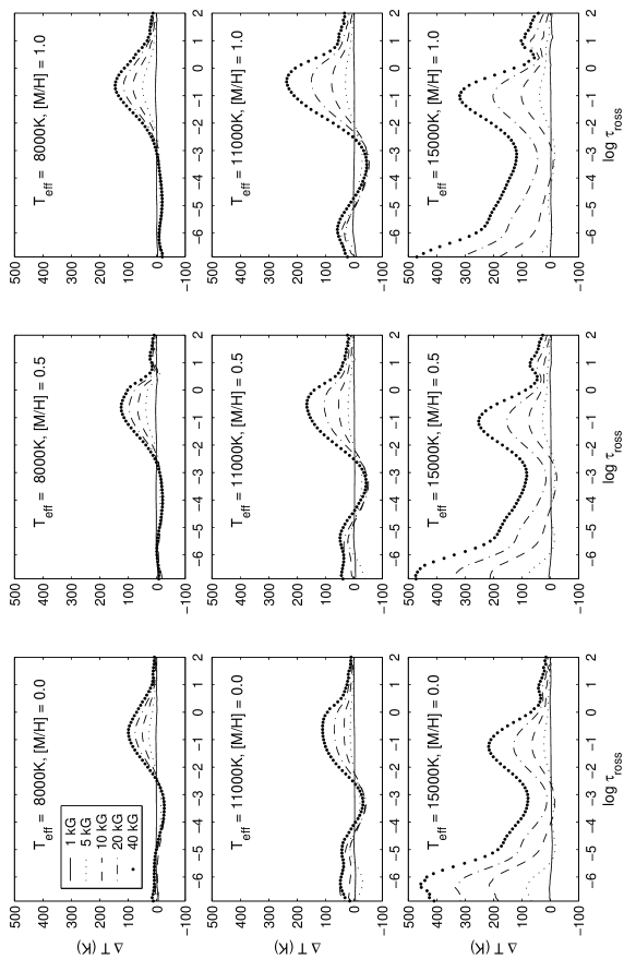
Figure 1: Difference of temperature between magnetic and non-magnetic model atmospheres for the effective temperatures ${T_{\rm eff}=8000}$ K, 11 000 K, 15 000 K and metallicities ${[M/H]=0.0}$, +0.5, +1.0.

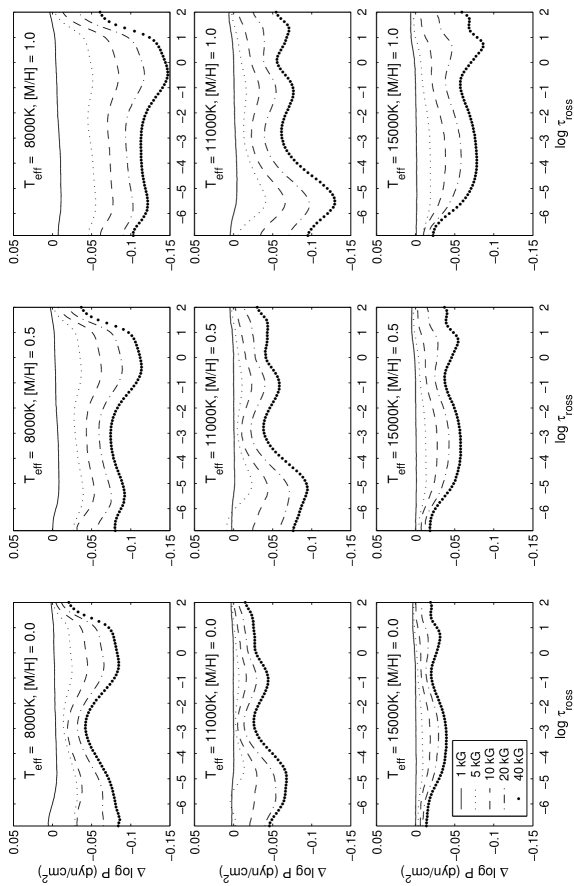
Figure 2: Difference of pressure between magnetic and non-magnetic model atmospheres for the effective temperatures ${T_{\rm eff}=8000}$ K, 11 000 K, 15 000 K and metallicities ${[M/H]=0.0}$, +0.5, +1.0.

3 Numerical results

Using the LLModels code and treating the magnetic opacity as detailed above, we have calculated a set of model atmospheres with the effective temperature ${T_{\rm eff}=8000}$ K, 11 000 K, 15 000 K, surface gravity $\log g=4.0$, metallicity $[M/H]=0.0$, +0.5, +1.0 and magnetic field strength 0, 1, 5, 10, 20 and 40 kG. For a few models with $[M/H]=+1.0$ we also considered the enhanced chromium abundance of $[Cr]=+2.0$ typical for some of the Cr-peculiar stars. The model atmosphere grid investigated in this paper covers substantial part of the stellar parameter space occupied by the magnetic Ap and Bp stars.

The model atmosphere calculations were carried out on the Rosseland optical depth grid spanning from $+2$ to $-6.875$ in $\log\tau_{\rm ross}$ and subdivided into 72 layers. Convection was neglected, since it is generally believed that strong global magnetic fields inhibit turbulent motions in the atmospheres of peculiar stars. Due the assumed absence of convection and because of a direct inclusion of the magnetic intensification in the modelling of spectral lines, we adopted zero microturbulent velocity in all calculations with magnetic field. A possibility to use pseudo-microturbulent velocity to mimic the effects of magnetic field on the line opacity was investigated by computing several model atmospheres with zero field and microturbulence in the range between 1 and 8 km s^-1.

Numerical tests demonstrated that a sufficient accuracy of the flux integration is achieved by using the following wavelength ranges for the spectrum synthesis: from 500 Å to 50 000 Å for ${T_{\rm eff}=8000}$ K, from 500 Å to 30 000 Å for ${T_{\rm eff}=11\,000}$ K and from 100 Å to 30 000 Å for ${T_{\rm eff}=15\,000}$ K. For all models we used a wavelength step of 0.1 Å, which resulted in the total number of frequency points in the range between 295 000 and 495 000.

At the first stage of creating models for each of the studied $T_{\rm eff}$, $[M/H]$ pairs we have used a standard atlas9 (Kurucz, 1993) model atmosphere for the spectral line preselection and as an initial guess of the model structure. The line selection threshold was set to 1%. Experiments with the smaller selection cutoffs in the range from $10^{-4}$% to 0.5% showed that, whereas including a larger number of lines results in a considerable increase of computing time, it leads to no more than 20–30 K difference of the temperature in the surface layers.

Two different initial approximations were investigated for calculation of magnetic model atmospheres. The first one uses a model atmosphere with zero magnetic field, whereas in the second one a new model is calculated using a converged model with a weaker field strength (i.e. the 0 kG model is used as an initial guess for the 1 kG model, then the 5 kG model is calculated starting from the 1 kG model, etc.). We found that the results of the two approaches are identical, but the second one requires far less computing time due to a faster convergence. Consequently, this iterative approach was used for the calculation of the magnetic model atmosphere grid presented here.

In the following sections we study the influence of the magnetic line blanketing on the model temperature and pressure structure and then investigate the effects on the common photometric and spectroscopic observables: spectral energy distribution, photometric colors in the Strömgren, Geneva and $\Delta a$ systems and profiles of the hydrogen Balmer lines.

3.1 Model structure

In Fig. 1 we show the difference between the temperature of magnetic and non-magnetic models as a function of the optical depth. The magnetic line blanketing typically increases temperature in the line forming region. This distortion becomes more pronounced in a stronger field and higher metal abundance. The most persistent effect of including magnetic field in the line opacity calculation is the heating of atmosphere in the optical depth range from $\log\tau_{\rm ross}=-2$ to 1. This phenomenon appears due to the enhanced line blanketing resulting from the additional absorption in Zeeman components. The additional opacity leads to a redistribution of the absorbed energy back to the lower atmospheric layers and, thus, to heating of the $\log\tau_{\rm ross}\approx-2\div 1$ region. This effect is present for all the models shown in Fig. 1.

In contrast, the behaviour of the upper layers depends strongly on the model parameters. For coolest stars considered here (${T_{\rm eff}=8000}$ K) we obtain a decrease of temperature in the upper layers. For the ${T_{\rm eff}=11\,000}$ K models this cooling is limited to a small range of depths centred at $\log\tau_{\rm ross}\approx-3.5$, whereas the magnetic models computed for ${T_{\rm eff}=15\,000}$ K display a significant increase of temperature throughout the atmosphere. This behaviour is explained by the shift from visual to UV of the wavelength interval which plays the most important role for the atmospheric energy balance. For the hotter models the line density in UV becomes very high due to Zeeman splitting and, therefore, even relatively high layers become opaque and are able to absorb additional incoming radiation and contributes to blanketing effect.

The pressure difference between magnetic and non-magnetic model atmospheres is shown in Fig. 2. The pressure stratification generally follows the tendencies of the temperature distribution: deviations from the non-magnetic models become larger with higher metal abundance and stronger magnetic field. The pressure tends to decrease when magnetic effects on the line opacity are taken into account. This is a consequence of a non-linear response of the model structure to the modification of the line opacity and the respective temperature increase due to the anomalous blanketing.

3.2 Energy distribution

The spectral energy distributions for the three values of effective temperature and metal overabundance of $[M/H]=+0.5$ and $[M/H]=+1.0$ are presented in Fig. 3. The theoretical energy distributions for magnetic stars are compared with the calculation for the reference non-magnetic models.

Three main anomalies are evident in the computed flux distribution of magnetic stars. The most conspicuous signature of the magnetically modified line blanketing is a flux deficiency in the ultraviolet spectral region and the respective flux excess in the visual. The magnitude of the UV deficiency is a moderate function of the effective temperature and clearly increases with the magnetic field strength and metallicity.

The presence of a magnetic field changes the stellar flux distribution in opposite direction in the visual and UV regions. At short wavelengths magnetic star appears to be cooler in comparison with a non-magnetic object with the same fundamental parameters, whereas in the visual magnetic star mimics a hotter normal star. The “null wavelength” where flux remains constant progressively shifts to bluer wavelengths as the stellar effective temperature increases.

Finally, we find that some of the theoretical flux distributions of magnetic stars exhibit depression in the 5200 Å region. This spectral feature has a well-known counterpart frequently observed in the spectra of peculiar stars (Kupka et al., 2003). In our theoretical calculations the 5200 Å depression is prominent at lower $T_{\rm eff}$ but becomes rather small for hotter models. The magnitude of the depression increases with the magnetic field intensity and metal content of the stellar atmosphere.

Figure 3: Synthetic energy distributions from UV to near IR region for effective temperatures ${T_{\rm eff}=8000}$ K, 11 000 K, 15 000 K and metallicities $[M/H]=+0.5$, $[M/H]=+1.0$. To enable visual comparison of the different curves the original LLModels stellar fluxes were convolved with a Gaussian profile with $FWHM=15$ Å. The insets show energy distributions in the 5200 Å region.

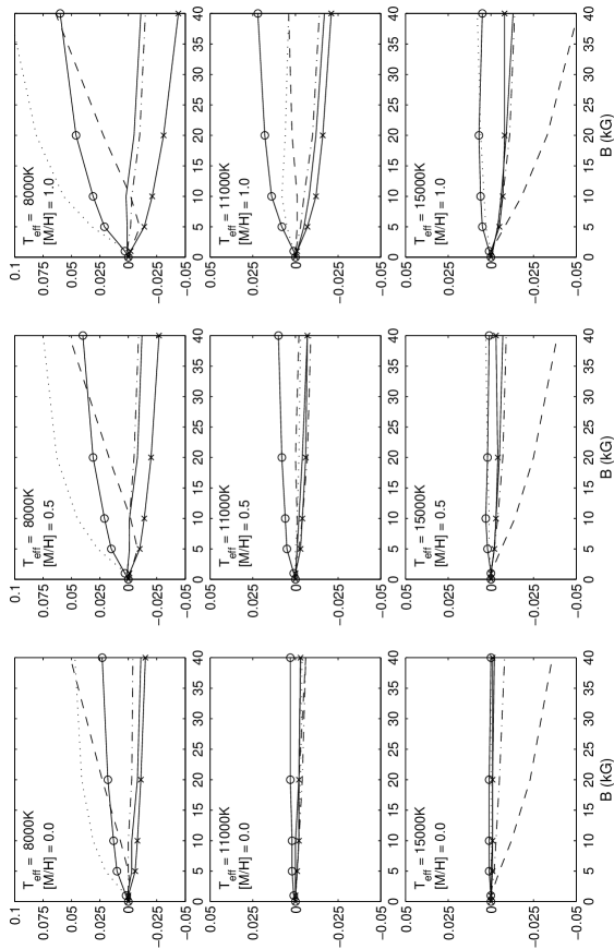
Figure 4: Difference between photometric color indices of magnetic stars in comparison with the predictions for the non-magnetic reference models. Effect of magnetic field on the photometric parameters of the Strömgren system is shown for $b-y$ (solid line), $m_{1}$ (dotted line), $c_{1}$ (dashed line) and $H\beta$ (dash-dotted line). The peculiarity indicators in the Geneva system, $\Delta(V_{1}-G)$ and $\Delta Z$, are shown with open circles and crosses respectively.

3.3 Colors

We studied the influence of the magnetic line blanketing on the photometric colors in the Strömgren $uvbyH\beta$, Geneva and $\Delta a$ systems. The dependence of various photometric parameters on magnetic field strength is shown in Figs. 4 and 5.

All colors were calculated using modified computer codes by Kurucz, (1993), which take into account transmission curves of individual photometric filters, mirror reflectivity and a photomultiplier response function. In contrast to the Kurucz’s procedures (Relyea & Kurucz, 1978) which are based on the low-resolution theoretical fluxes, our synthetic colors are computed from the energy distributions sampled every 0.1Å, so integration errors are expected to be small.

The peculiar parameter $\Delta a$ was introduced by Maitzen, (1976) to measure the strength of the 5200 Å depression. Our calculations of the synthetic $\Delta a$ photometry were carried out using the tabulated filter transmission curves and the photomultiplier response functions as discussed in the recent paper by Kupka et al., (2003). In addition, the peculiarity parameters $Z$ and $\Delta(V_{1}-G)$ of the Geneva photometric systems were computed according to Cramer & Maeder, (1979).

As one expects, the behaviour of the photometric indices is closely related to the flux redistribution between the visual and UV regions and the presence of several flux depressions, such the one at 5200 Å. The shift of the “null wavelength” leads to alternation of the Balmer discontinuity amplitude as measured by the $c_{1}$ index of the $uvbyH\beta$ system (see Fig. 4). We found that for all metallicities a relation between $c_{1}$ and the magnetic field intensity is almost linear for ${T_{\rm eff}=8000}$ K and ${T_{\rm eff}=15\,000}$ K, with positive and negative correlation respectively. On the other hand, for ${T_{\rm eff}=11\,000}$ K the $c_{1}$ index does not show any trend with the magnetic field strength because for this temperature the flux increases by a similar amount on both sides of the Balmer jump.

A relation between changes of all photometric indices and the intensity of magnetic field depends strongly on the stellar effective temperature. For low $T_{\rm eff}$ photometric changes are very pronounced, whereas for hotter magnetic stars modification of the $uvbyH\beta$ photometric observables is fairly small (except $c_{1}$). The Geneva photometric colors show a similar decrease of the sensitivity to the magnetic effects with increasing $T_{\rm eff}$. This picture agrees with the general temperature behaviour of the theoretical flux distributions evident in Fig. 3.

The $\Delta a$ photometric system, characterizing the strength of the 5200 Å depression, has long been considered as one of the most useful peculiarity indicators for stars with non-solar chemical composition and strong magnetic field (e.g., see Kupka et al. 2003, 2004 and references therein). Results of our calculations of the synthetic $\Delta a$ parameter are summarized in Fig. 5 and confirm its sensitivity to the metal abundance and magnetic field strength. However, similar to the effects observed for other medium and narrow-band photometric indicators, $\Delta a$ is most influenced by magnetic field at lower $T_{\rm eff}$, whereas the trend of $\Delta a$ vs. the field strength quickly saturates for higher temperatures. For example, for $T_{\rm eff}=8000$ K and $[M/H]=+1.0$ the $\Delta a$ index shows 0.043 mag difference between the 0 kG and 20 kG field strengths, for $T_{\rm eff}=11\,000$ K this difference decreases to 0.026 mag and it drops to 0.010 mag for the models computed with $T_{\rm eff}=15\,000$ K.

The prominent temperature sensitivity of the behaviour of the synthetic $\Delta a$ indices arises because the absorption in the 5200 Å region is dominated by the Fe i and low excitation Fe ii lines. These features become weaker with increasing $T_{\rm eff}$, hence the depression is stronger and more sensitive to the field strength in cooler magnetic stars.

All photometric indices become more sensitive to the magnetic effects with increasing metallicity. This is most clearly visible for the $\Delta a$ index computed for $T_{\rm eff}=8000$ and 11 000 K models. The respective panels in Fig. 5 demonstrate that, for instance, the difference between $\Delta a$ values for the models with ${T_{\rm eff}=8000}$ K, ${[M/H]=0.0}$ and ${[M/H]=+1.0}$ increases from the initial 0.010 mag for zero field to 0.031 mag for $B=40$ kG. This effect is even more dramatic for ${T_{\rm eff}=11\,000}$ K where the difference $\Delta a_{[M/H]=+1.0}-\Delta a_{[M/H]=0.0}$ grows from 0.016 to 0.041 mag.

Figure 5: The magnitude of the $\Delta a$ photometric index as a function of the magnetic field strength for $T_{\rm eff}=8000$, 11 000 and 15 000 K. Different curves show calculations with metal abundances $[M/H]=0.0$ (open circles), $[M/H]=+0.5$ (triangles) and $[M/H]=+1.0$ (filled circles). Open squares illustrate the effect of increasing Cr overabundance to $[Cr]=+2.0$ in the $T_{\rm eff}=8000$, $[M/H]=+1.0$ models.

An anomalous concentration of individual species with abundant spectral lines may have important implications for the $\Delta a$ value. For the models with scaled solar abundance the 5200 Å depression is produced mainly by the Fe lines. Contribution of the lines of other elements becomes significant only when the respective species are strongly overabundant. As illustrated in Fig. 5, increasing the Cr overabundance by a factor of 100 relative to the sun results in 0.016–0.023 mag growth of the $\Delta a$ index for ${T_{\rm eff}=8000}$ K, ${[M/H]=+1.0}$ model and the field strength 5–20 kG.

Hauck, (1974) has demonstrated that the $\Delta(V_{1}-G)$ index of the Geneva system could be used as a peculiarity parameter for Ap stars. We found that the behaviour of $\Delta(V_{1}-G)$ is comparable to that of the $\Delta a$ index. The maximum change of the $\Delta(V_{1}-G)$ parameter relative to the non-magnetic case is 0.060 mag for ${B=40}$ kG, ${T_{\rm eff}=8000}$ K and ${[M/H]=+1.0}$.

The $X$, $Y$, $Z$ parameters introduced by Cramer & Maeder, (1980) are linear combinations of the Geneva photometric indices. The $Z$ value was suggested to be an indicator of chemical peculiarity and the strength of the surface magnetic field (North, 1980). We found that the maximum change of $Z$ relative to the non-magnetic case equals to $-0.044$ mag for ${T_{\rm eff}=8000}$ K, ${[M/H]=+1.0}$ and ${B=40}$ kG. However, at higher temperatures $Z$ becomes less sensitive to the magnetic field effects compared to $\Delta(V_{1}-G)$ and $\Delta a$.

Finally, we note that none of the photometric indicators of magnetic stars proposed in the literature shows a linear trend over the whole range of the considered magnetic field strength. Relations between changes of the photometric indices and the magnetic field intensity show saturation effects for ${B\gtrsim 10}$ kG. This saturation can be offset to stronger fields by increasing the number of spectral lines affected by the Zeeman splitting and intensification, which explains greater magnetic sensitivity of the synthetic photometry computed for the models with lower $T_{\rm eff}$ and higher metal abundance.

3.4 Hydrogen line profiles and metal lines

Profiles of the H$\alpha$, H$\beta$ and H$\gamma$ hydrogen Balmer lines were calculated using the Synth program (Piskunov, 1992). This spectrum synthesis code incorporates the new hydrogen line Stark broadening computations by Stehlé, (1994), as well as the improved treatment of the hydrogen line self-broadening developed by Barklem et al., (2000). The comparison between the magnetic and non-magnetic profiles of the H$\beta$ line calculated for models with 10 times the solar metal abundance is presented in Fig. 6.

We found that the changes in the atmospheric structure due to the magnetic line blanketing do not have a strong influence on the hydrogen line profiles. For H$\beta$ the maximum change relative to the non-magnetic model amounts to about 3% of the continuum level for ${B=40}$ kG, but it does not exceed 1% for $B\leq 10$ kG, which is a more typical surface field strength for the majority of magnetic CP stars.

To estimate an effect of the anomalous atmospheric structure of the magnetic models on the profiles of individual metal lines we computed synthetic spectra in the 4000–6000 Å region for the zero field and the 10 kG field models and $[M/H]=+1.0$. Since at this point we are interested to study only the effects of the model structure, the spectrum synthesis calculations were carried out disregarding magnetic field. We found that the depth of absorption lines is modified in the spectra computed with the magnetic models. The strongest effect is found for $T_{\rm eff}=8000$ K, where in the presence of the 10 kG field many medium strength and weak lines become sytematically shallower by 4–6% of the continuum level relative to the calculation with the zero field model. This discrepancy is reduced to less than 2–3% for the $T_{\rm eff}=11\,000$ and 15 000 K models. For these hotter atmospheres the difference between the line profiles computed for the magnetic and non-magnetic models can be both negative and positive. For many lines the main discrepancy is concentrated in the line wings, with the magnetic models predicting slightly narrower line profiles.

Figure 6: Comparison between the synthetic H$\beta$ profiles computed for ${[M/H]=+1.0}$ and different values of the magnetic field strength and $T_{\rm eff}$. The lower panels show normalized profiles, whereas the upper plots illustrate the difference between H$\beta$ calculated for the models with substantial magnetic line blanketing and the reference non-magnetic model.

3.5 Stellar atmospheric parameters and bolometric correction

The overall modification of the energy distribution of magnetic stars as well as the presence of localized absorption features may bias photometric determination of the stellar atmospheric parameters. As a part of the investigation in this paper, we verified an influence of the magnetic line blanketing on the photometric determination of $T_{\rm eff}$ and $\log g$.

The TempLogg code (Rogers, 1995) was applied to the synthetic $uvbyH\beta$ colors calculated as described in Sect. 3.3. We found that for ${T_{\rm eff}=8000}$ K the maximum difference between $T_{\rm eff}$ and $\log g$ obtained for non-magnetic models and the corresponding parameters for the ${B=40}$ kG models is $-190$ K and $-0.27$ dex respectively. For the ${T_{\rm eff}=11\,000}$ K models the temperature discrepancy is maximal ($+$86 K) for normal composition and decreases with increasing metal abundance, whereas the difference of $\log g$ peaks at $-0.11$ dex. For the hottest models ($T_{\rm eff}=15\,000$ K) the $T_{\rm eff}$ difference is $+541$ K, but $\log g$ is not affected. It is clear that, even in the case of extreme magnetic field strengths, the bias in determination of the fundamental parameters using the Strömgren photometry does not result in a systematic deviation of $T_{\rm eff}$ and $\log g$ beyond the usual error bars assigned to the photometrically determined stellar parameters.

Somewhat different results emerged from our analysis of the stellar parameters determined using the Geneva photometric system. Effective temperature was derived applying the code of Künzli et al., (1997) to the synthetic Geneva colors and was found to increase systematically with the field strength for all three considered $T_{\rm eff}$ values. The bias introduced by magnetic field reaches 100–200 K for ${T_{\rm eff}=8000}$–11 000 K and 900 K for ${T_{\rm eff}=15\,000}$ K. The surface gravity is modified by up to 0.2 dex. Thus, a higher sensitivity to the metallic line absorption makes the standard Geneva photometric calibration a less robust method for determination of the atmospheric parameters of magnetic stars compared to the calibration in terms of the $uvbyH\beta$ colors.

An increase of the line blanketing due to magnetic effects and overabundance of metals lead to a redistribution of the stellar flux from UV to visual. Consequently, magnetic CP stars appear brighter in $V$ compared to normal stars with the same fundamental parameters. Using the theoretical flux distributions calculated with the LLModels code we studied the effect of magnetic field and metallicity on the bolometric correction (BC). For all stellar models this parameter decreases relative to the non-magnetic case by up to 0.054–0.089 mag for $B=40$ kG and by no more than 0.025 mag for $B\leq 10$ kG. The BC for the ${T_{\rm eff}=15\,000}$ K models is the most sensitive to magnetic field. At the same time, even in the absence of the field, an increase of metal abundance leads to a substantial modification of BC. It decreases by 0.079–0.115 mag when metal abundance is changed from solar to $[M/H]=+1.0$.

3.6 Enhanced microturbulence models

Until the present investigation the most common approach to account for the magnetic line blanketing in the model atmosphere analyses of magnetic CP stars was to use an increased value of the microturbulent velocity (Muthsam, 1979; Kupka et al., 2004). For the magnetic field $B$ such a pseudomicroturbulent velocity is computed according to the following equation (e.g., Kupka et al. 1996):

$$\xi_{\rm mag}=4.66\times 10^{-13}c\,\lambda g_{\rm eff}B,$$ (8)

where $c$ is the speed of light in km s^-1, the field strength $B$ is measured in gauss, $\lambda$ is the wavelength in Å and $g_{\rm eff}$ is the effective Landé factor. In previous model atmosphere studies $\lambda\approx 5000$ Å and $g_{\rm eff}=1.0$–1.2 were typically adopted, which gives $\xi_{\rm mag}\approx 4$ and 8 km s^-1 for the magnetic field strength of 5 and 10 kG respectively.

Having introduced a more realistic implementation of the magnetic intensification in modelling of stellar atmospheres, we are in the position to verify the extent to which models with the magnetic pseudomicroturbulence are able to match the properties of our more sophisticated but, admittedly, also more computationally expensive models. To study the performance of the enhanced microturbulence models, the model structure, energy distribution and synthetic $\Delta a$ indices computed for zero field and $\xi_{\rm mag}=1$–8 km s^-1 were compared with the respective parameters for the $B=5$ and 10 kG models from our main grid.

It appears that the enhanced microturbulence is indeed able to partially mimic the behaviour of magnetic models, such as the energy redistribution from UV to visual and the heating in certain atmospheric layers. However, an exact quantitative match requires adopting a different $\xi_{\rm mag}$ parameter for each considered quantity. For instance, to reproduce the temperature structure and energy distribution of the $T_{\rm eff}=8000$ K models one has to use (depending on metallicity) $\xi_{\rm mag}=2.1$–2.6 km s^-1 and 3.7–4.1 km s^-1 for $B=5$ and 10 kG respectively, which is roughly a factor of two smaller microturbulence than predicted by Eq. (8). At the same time, matching the anomalous absorption in the 5200 Å region requires a 2–3 km s^-1 higher value of $\xi_{\rm mag}$. Furthermore, models’ sensitivity to the magnetic line blanketing decreases with $T_{\rm eff}$ faster than the influence of microturbulence. Consequently, for the $T_{\rm eff}=15\,000$ K models one has to adopt nearly twice as weaker $\xi_{\rm mag}$ to simulate effect of the same field as in cooler models.

Results of the calculations in this section demonstrate that a properly chosen value of $\xi_{\rm mag}$ can only be used as a very rough guess of the effects due to magnetic field. However, it is evident that the models with enhanced microturbulence are not suitable for detailed analysis of magnetic stars and cannot be used for modelling individual features of the stellar flux distributions.

4 Conclusions and discussion

Construction of the model atmospheres of CP stars is considerably more complicated in comparison to that of normal stars because such modelling has to take into account and explain a range of phenomena not present in the atmospheres of normal stars. The main and most important distinction of magnetic CP stars from the other Main Sequence objects is the presence of a strong global magnetic field. It plays a central role in producing chemical abundance anomalies and inhomogeneities and leads to a peculiar atmospheric structure, unusual line profiles and an anomalous flux distribution.

The Zeeman splitting of spectral lines is one of the principal effects taking place in the magnetic stellar atmosphere. In this study we have computed a grid of model atmospheres of peculiar A and B stars accounting for the magnetic line blanketing. Our model grid has covered the range of possible atmospheric parameters of CP stars, which allowed us to analyze the behaviour of the model structure and observed characteristics for different magnetic field, abundances and effective temperature. We have used the new model atmosphere code LLModels and up-to-date compilations of the atomic line data from the VALD database to insure an accurate modelling.

A somewhat simplified “horizontal” model of magnetic field allowed us to reduce computational costs by solving the radiative transfer equation for the non-polarized radiation. This approach does not fully reflect the influence of magnetic field on the formation of spectral lines but, nevertheless, it represents the most accurate treatment of the Zeeman effect in model atmosphere calculation used so far.

Our models show that the enhanced line blanketing due to the magnetic intensification of spectral lines produces heating of the certain atmospheric layers and this effect increases with effective temperature, magnetic field strength and metal abundance.

We found that the model atmospheres with the magnetic line blanketing produce fluxes that are deficient in the UV region by ${0.2-0.3}$ mag for ${B=10}$ kG and about ${0.3-0.8}$ mag for ${B=40}$ kG. Moreover, the presence of a magnetic field leads to the flux redistribution from the UV to visual region due to backwarming. This property of the theoretical models is in agreement with those observations of CP stars (Leckrone, 1974; Molnar, 1973; Jamar, 1977) which have revealed the presence of the flux redistribution and demonstrated that the flux changes in the visible and ultraviolet regions are inversely correlated.

The energy distributions of the calculated model atmospheres show that an increase of effective temperature shifts the “null wavelength” where flux remains unchanged to shorter wavelengths. The results of our modelling suggest that the “null wavelength” approximately falls at 3800 Å for ${T_{\rm eff}=8000}$ K, at 2900 Å for ${T_{\rm eff}=11\,000}$ K and at 2600 Å for ${T_{\rm eff}=15\,000}$ K and slightly depends on metallicity and field strength. This fact is in concordance with the observational data and numerical experiments by Leckrone et al., (1974) who examined enhanced opacity models and found that the “null wavelength” shifts toward UV when effective temperature is increased.

Magnetic CP stars demonstrate several flux depressions in the visual and ultraviolet region unlike other stars. The most prominent feature in the visual is the flux depression centred at 5200 Å. Our numerical results show that the strong feature near 5200 Å appears for lower effective temperature and vanishes for higher effective temperature and its amplitude increases with the magnetic field strength and metallicity. Comparison of the synthetic $\Delta a$ indices with typical values of this parameter observed for cool magnetic stars demonstrate that our calculation are able to reproduce the whole range of the 5200 Å depression strength. Furthermore, our results argue that for modelling the 5200 Å feature in cool CP stars an accurate treatment of magnetic field is of no less importance compared to using individual abundances (Kupka et al., 2004). A 10 kG magnetic field changes the value of the $\Delta a$ parameter by as much as 20–30 mmag, which is substantial even compared to the largest observed $\Delta a$ values.

Since, historically, photometric data are widely used for the stellar classification and atmospheric parameter determination, we have calculated indices in the $uvbyH\beta$ and Geneva photometric systems as well as the peculiar indices $\Delta a$, $Z$ and $\Delta(V_{1}-G)$. We found that changes of most photometric parameters due to the influence of magnetic field are noticeable for low effective temperatures, whereas for hotter stars sensitivity to magnetic field is reduced considerably. This behaviour of the theoretical models agrees with the flux distribution properties and with the study by Cramer & Maeder, (1980), who noted that the effects of magnetic field on the energy distribution become less important with an increase of temperature.

The peculiar indices $\Delta a$, $Z$ and $\Delta(V_{1}-G)$ are frequently used for identification and assessment of the properties (in particular the surface field strength) of CP stars. We examined the influence of magnetic field on these indices. We found that the magnetic modification of the peculiar photometric parameters is relatively small (maximum change of $\Delta a$ is 0.065 mag for 40 kG field) and the relation between their values and the magnetic field strength is not linear due to the saturation effects for stronger field (${B\gtrsim 10}$ kG). In any case, the $\Delta a$ parameter appears to be the most sensitive to magnetic field, whereas $Z$ and $\Delta(V_{1}-G)$ are less sensitive. Cramer & Maeder, (1980) pointed that the saturation of the photometric effects for large fields is an observational fact and has to be explained by a model atmosphere analysis. Our numerical results reproduce and provide a clear explanation of the behaviour of the photometric indices.

Finally, we investigated the question to what extent the anomalous magnetic opacity affects the photometric determination of the atmosphere parameters of CP stars. We found that, although an enhanced metal abundance and magnetically modified line opacity produce some changes of the model atmosphere structure and the flux distribution, these changes are not very large and do not result in a strong modification of the optical photometric colors. Consequently, the model atmosphere parameters derived using the photometric calibrations for normal stars are not far from their true values. Thus, despite the presence of several local anomalies of the stellar energy distribution and the overall flux redistribution from the UV to visual region, peculiar stellar models do not appear to mimic standard models with a systematically different $T_{\rm eff}$. Standard calibrations of the Strömgren photometry appear to be especially robust for the determination of the parameters of magnetic stars. Thus, we conclude that by itself the magnetic opacity does not introduce significant errors in the photometric estimates of CP-star parameters.

We also showed that the hydrogen Balmer line and absorption features of metals are not very sensitive to the changes induced by the magnetic line blanketing on the model atmosphere structure. Although the effect on the overall flux distribution may be noticeable, the changes in the depths of metal lines do not exceed a few % of the continuum level for the 10 kG field, which justifies neglecting magnetic line blanketing in the routine abundance and spectrum synthesis studies of the majority of magnetic CP stars.