Bypass to Turbulence in Hydrodynamic Accretion: Lagrangian Analysis of Energy Growth

Abstract

Despite observational evidence for cold neutral astrophysical accretion disks, the viscous process which may drive the accretion in such systems is not yet understood. While molecular viscosity is too small to explain the observed accretion efficiencies by more than ten orders of magnitude, the absence of any linear instability in Keplerian accretion flows is often used to rule out the possibility of turbulent viscosity. Recently, the fact that some fine tuned disturbances of any inviscid shear flow can reach arbitrarily large transient growth has been proposed as an alternative route to turbulence in these systems. We present an analytic study of this process for 3D plane wave disturbances of a general rotating shear flow in Lagrangian coordinates, and demonstrate that large transient growth is the generic feature of non-axisymmetric disturbances with near radial leading wave vectors. The maximum energy growth is slower than quadratic, but faster than linear in time. The fastest growth occurs for two dimensional perturbations, and is only limited by viscosity, and ultimately by the disk vertical thickness.

After including viscosity and vertical structure, we find that, as a function of the Reynolds number, ${\cal R}$, the maximum energy growth is approximately $0.4({\cal R}/\log{\cal R})^{2/3}$, and put forth a heuristic argument for why ${\cal R}\gtrsim 10^{4}$ is required to sustain turbulence in Keplerian disks. Therefore, assuming that there exists a non-linear feedback process to replenish the seeds for transient growth, astrophysical accretion disks must be well within the turbulent regime. However, large 3D numerical simulations running for many orbital times, and/or with fine tuned initial conditions, are required to confirm Keplerian hydrodynamic turbulence on the computer.

1 Introduction

Accretion disks are very common in astrophysics. Disks are found in Active Galactic Nuclei (AGN), around newly forming stars (proto-planetary disks), and surrounding compact stellar remnants (white dwarfs, neutron stars, black holes) in binary systems (e.g., Pringle, 1981). Despite the overwhelming evidence for the existence of accretion disks (e.g., Lin & Papaloizou, 1996), and decades of literature dedicated to their understanding (e.g., see Balbus & Hawley, 1998, and references therein), the detailed working mechanism of accretion disks remains enigmatic at best.

One of the early puzzles in understanding the accretion phenomenon was the clear inadequacy of molecular viscosity in driving accretion in a Keplerian disk. This led to the speculation of turbulence as a proxy for viscous transfer of angular momentum (Weizsacker, 1948; Shakura & Sunyaev, 1976). The idea was particularly attractive because of the low viscosity of astrophysical fluids (high Reynolds number $\sim 10^{10}-10^{14}$), which, according to conventional wisdom, should make the shear flow in accretion disks unstable to turbulence.

However, in the context of Keplerian disks relevant to most astrophysical applications, no instability could be identified. The linear instabilities that seemingly induce the onset of turbulence in normal shear flows are stabilized by the Coriolis force associated with rotation in a Keplerian disk. Nonlinear hydrodynamic simulations appeared to confirm the absence of turbulence in such disks (Balbus, Hawley, & Stone, 1996; Hawley, Balbus, & Winters, 1999, both hereafter referred to as BHSW).

The breakthrough came in 1991, through re-discovery of the Magnetorotational Instability (MRI; Chandrasekhar, 1960) by Balbus and Hawley (Balbus & Hawley, 1991), who showed through Magnetohydrodynamic (MHD) simulations that initial seed magnetic fields in an MHD disk grow exponentially within a few rotation times, causing the onset of MHD turbulence. The MRI instability is now widely accepted as the driver of MHD turbulence in ionized disks (see e.g., Balbus, 2003, for a recent review).

Despite the great success of the MRI in many astrophysical systems, it is known that this instability will not operate in disks with very small ionization fractions, where the magnetic flux is poorly coupled to the gas. Examples of systems with low ionization fractions are proto-planetary disks, outer regions of AGN disks, and white dwarf disks in the low state (Gammie, 1996; Gammie & Menou, 1998; Formang, Terquem, & Balbus, 2002). The route to turbulence and accretion in such neutral disks remains an outstanding puzzle in theoretical astrophysics.

On the other hand, laboratory experiments of Taylor-Couette systems (fluid flow between concentric rotating cylinders) seem to indicate that, although Coriolis force delays the onset of turbulence, the flow is ultimately unstable to turbulence for Reynolds numbers larger than a few thousand (e.g., see Richard, 2001), even for subcritical systems (systems with no linear instability). Longaretti (2002) reviews the experimental evidence for the existence of turbulence in subcritical laboratory systems, and based on phenomenological analogy, concludes that a similar process must happen in astrophysical accretion flows. Longaretti (2002) also claims that the absence of turbulence in previous numerical simulations (BHSW) is due to their small effective Reynolds number, which is limited by the numerical viscosity caused by the finite resolution of the simulation. Indeed, Bech & Andersson (1997) see turbulence persisting in numerical simulations of subcritical rotating flows for large enough Reynolds numbers.

How does a shearing flow that is linearly stable to perturbations switch to a turbulent state? A possible explanation, known as bypass transition, has been discussed in the fluid mechanics community for some time (see Grossmann, 2000; Reshotko, 2001; Schmid & Henningson, 2000, and references therein, for an overview), though its diffusion into the astrophysical community has been slow (Ioannou & Kakouris, 2001; Chagelishvili et al., 2003; Tevzadze et al., 2003; Yecko, 2004; Umurhan & Regev, 2004). The bypass concept is based on the fact that definite frequency linear modes are not orthogonal in a shear flow. Therefore, even if all of the linear modes are decaying, a suitably tuned linear combination of them can still show an arbitrarily large transient energy growth in the absence of viscosity. In lieu of linear instabilities such as MRI, the transient energy growth, supplemented by a non-linear feedback process to repopulate the growing disturbances, could plausibly sustain turbulence for large enough Reynolds numbers.

This paper, along with a companion paper (Mukhopadhyay, Afshordi, & Narayan, 2004, hereafter MAN04), investigates the transient growth of perturbations in rotating shear flows, with an emphasis on applications to astrophysical accretion disks. Both papers study the dependence of the transient energy growth on various parameters of the system, in particular the wave vector of the perturbations and the Reynolds number. While MAN04 focuses on an eigenmode analysis in Eulerian coordinates for a shearing flow restricted between rigid walls, the present paper studies the bypass process in Lagrangian coordinates for an infinite shearing flow. The advantage of the Lagrangian approach is that there is no explicit coordinate dependence in the equations, and therefore the solution can be decomposed into plane waves. The drawback, however, is the explicit time dependence of the equations which prohibits definite frequency solutions, and thus requires explicit integration in time for each mode. The two analyses presented here and in MAN04 involve different numerical/analytic techniques and are both, in our opinion, valuable. The consistency of the results validates the general picture of our understanding of transient growth in the linear regime.

In §2 we summarize the current understanding of the transient growth phenomenon in shearing flows. §3 introduces the basic linear equations in Lagrangian coordinates in their most general form. §4 constitutes the main body of the paper, where we approach the problem of transient growth in inviscid and incompressible flows for general plane wave solutions. This is followed by §5 and §6, where we study the effects of viscosity and compressibility/vertical structure, respectively, and make the connection to astrophysical accretion flows. Finally, in §7 we discuss conditions for the emergence of turbulence, and its realization in numerical simulations. §8 summarizes our results and concludes the paper.

2 Understanding Transient Growth through Swinging Plane Waves

As mentioned in §1, the systematic approach to transient growth in subcritical systems is through a linear combination of non-normal decaying modes. In particular, in a local region of an accretion flow, different definite frequency modes with equal vertical and azimuthal wave numbers, but different radial profiles, are generically not orthogonal to one another, i.e.

$$\int d^{3}{\bf x}~{}{\bf{\delta v}}^{a}\cdot{\bf{\delta v}}^{b}\neq 0,$$ (1)

where ${\bf{\delta v}}^{a}$ and ${\bf{\delta v}}^{b}$ are velocity profiles of different modes. Therefore, even though all the modes may decay with time, a solution may still show a temporary energy growth for suitable initial conditions because of the cross terms in the energy expression. For a detailed description of the eigenmode approach, we refer the reader to MAN04 and Yecko (2004), which explain the numerical methods used to find the maximum growth through optimizing a linear combination of eigenmodes.

An alternative approach, which allows simple analytic treatment of linear perturbations for the case of astrophysical accretion flows, is the so-called shearing box approximation in which we study the linear evolution of plane wave perturbations in Lagrangian coordinates within a small region of an accretion flow (Chagelishvili et al., 2003; Tevzadze et al., 2003; Umurhan & Regev, 2004). This is the approach we follow in this paper.

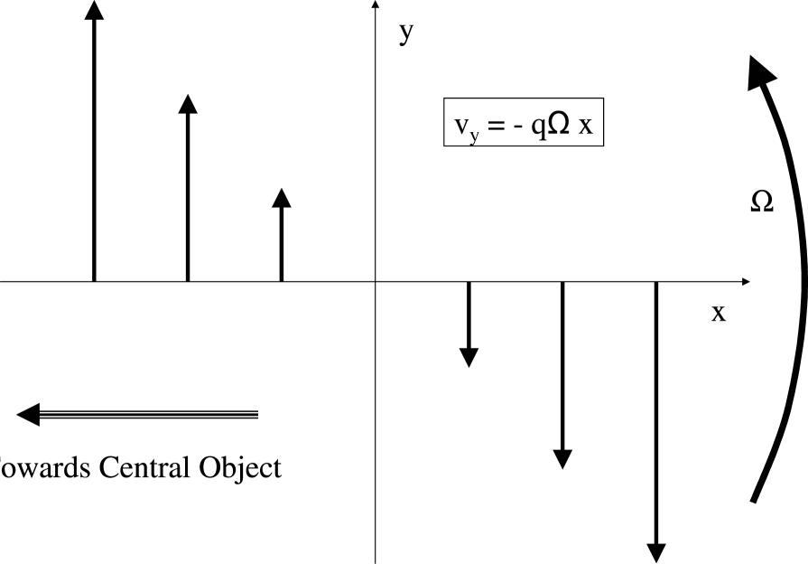
Figure 1: A plot of the unperturbed flow in the local comoving box studied in this paper. The thick arrows represent the velocity field.

Fig. 1 shows our choice of local Cartesian coordinates: $x$ is along the radial direction, $y$ is along the azimuthal or streamwise direction, and $z$ is along the vertical direction. The unperturbed flow has a velocity in the $y$-direction and a velocity gradient (shear) along the $x$ direction. The Coriolis force associated with rotation is described by an angular frequency vector ${\bf\Omega}$ pointed in the $z$ direction. We define

$$q\equiv-d\ln\Omega/d\ln R,$$ (2)

which is a dimensionless parameter that quantifies the shear in the local comoving box . For example, $q=3/2$ corresponds to a Keplerian accretion disk and $q=2$ to a disk with constant specific angular momentum.

Starting with a plane wave in Lagrangian coordinates with radial wave number $k^{L}_{x}$ (Eq. 16), we show in §3 that the Eulerian radial wave number $k_{x}$ of the plane wave evolves as a function of time $t$ according to:

$$k_{x}=k^{L}_{x}+(q\Omega t)k_{y},$$ (3)

while the azimuthal and vertical wave numbers $k_{y}$ and $k_{z}$ remain unchanged. Thus, the plane wave is effectively frozen into the flow and is swung around by the shear. For simplicity, as in Chagelishvili et al. (2003) and Umurhan & Regev (2004), let us consider ‘two-dimensional’ ($k_{z}=0$) incompressible and inviscid perturbations. In this regime, in general, the two-dimensional vorticity $\xi=k_{x}{\delta v}_{y}-k_{y}{\delta v}_{x}$ remains constant, while the two-dimensional divergence vanishes due to incompressibility, i.e. $k_{x}{\delta v}_{x}+k_{y}{\delta v}_{y}=0$. Therefore, the energy content of the plane wave scales as:

$${\cal E}\propto{\delta v}^{2}_{x}+{\delta v}^{2}_{y}=\frac{\xi^{2}}{k^{2}_{x}+k^{2}_{y}}=\frac{\xi^{2}}{\left[k^{L}_{x}+(q\Omega t)k_{y}\right]^{2}+k^{2}_{y}},$$ (4)

which reaches a maximum when $k_{x}=0$, or $k^{L}_{x}/k_{y}=-q\Omega t$. If the initial wave vector $k_{x}=k^{L}_{x}$ is negative, then the maximum is reached at positive time, and the energy growth factor is given by:

$$G_{max}\equiv\frac{{\cal E}_{max}}{{\cal E}(0)}\simeq(k^{L}_{x}/k_{y})^{2}=(q\Omega t)^{2}~{}{\rm for}~{}-k^{L}_{x}/k_{y}\gg 1.$$ (5)

As promised, the growth can become arbitrarily large for long enough time. As we show in §6, the maximum growth is limited only by viscosity and scales as ${\cal R}^{2/3}$, where ${\cal R}$ is the Reynolds number (Chagelishvili et al., 2003; Yecko, 2004, MAN04). Note that, after reaching the maximum, the linear solution drops and decays to zero asymptotically. Therefore, to have sustained turbulence, the perturbations must become non-linear before reaching the peak and must provide sufficient feedback to keep the perturbations going. Umurhan & Regev (2004) describe a 2D numerical simulation of the local accretion flow in which they find sustained turbulent behavior in the absence of viscosity.

Moving away from the $k_{z}=0$ plane, it is seen that for $q\lesssim 2$ (the regime of interest for astrophysical disks), the maximum growth drops (Yecko, 2004, MAN04). However, Tevzadze et al. (2003) argue that for $k_{z}\neq 0$, although the maximum growth is smaller, vertical stratification may cause the solution to have a non-vanishing asymptotic value, which is a fraction of the maximum growth. It is not clear if this will significantly help the onset of turbulence.

This concludes our summary of (the rather thin) astrophysical literature on transient growth and the bypass mechanism. In the following sections, we present a formal treatment of the Lagrangian hydrodynamic equations in the shearing box approximation, and study the transient growth of general plane wave solutions.

3 Hydrodynamic Equations in the Local Lagrangian Coordinates (Shearing Box Approximation)

We limit the calculations to scales much smaller than the thickness of the disk, which, for a geometrically thin disk, is in turn much smaller than the distance to the central object. We thus ignore the boundaries. Within a comoving local box, and in terms of Lagrangian coordinates, the Navier-Stokes and continuity equations can be written as:

$$\dot{\bf v} = -c^{2}_{s}{\bf\nabla}\lambda+\nu\nabla^{2}{\bf v}+2{\bf v\times\Omega},$$ (6)

$$\dot{\lambda} = -{\bf\nabla.v},$$ (7)

$$\dot{\bf r} = {\bf v}({\bf r}^{L}),$$ (8)

$${\bf\nabla} \equiv {\bf\partial r^{L}\over\partial r}{\bf.\nabla^{L}},$$ (9)

where ${\bf v}$ is the fluid velocity vector, ${\bf r}$ and ${\bf r}^{L}$ are Eulerian and Lagrangian position vectors respectively, $\nu$ is the kinematic coefficient of (molecular) viscosity, and $\lambda\equiv\ln\rho$ is the logarithm of fluid density. Since the local box rotates with the flow, we have a Coriolis term on the right hand side of the Navier-Stokes equation (6), which is proportional to the local angular velocity ${\bf\Omega}$; in the shearing box approximation, the Coriolis parameter $\Omega$ is taken to be independent of position. We have dropped the centrifugal and gravitational accelerations, as they cancel in the equilibrium flow and do not contribute to the perturbation equations.

Fig. 1 shows the unperturbed velocity field within the local comoving box. Let us define $\Omega{\mathfrak{q}}$ as minus the gradient of the unperturbed velocity field,

$$\Omega{\mathfrak{q}}\equiv-{\bf\nabla v}=-{(\bf\nabla\Omega)\times R}=\left(\begin{array}[]{ccc}0&q\Omega&0\\ 0&0&0\\ 0&0&0\end{array}\right);~{}~{}q=-\frac{d\ln\Omega}{d\ln R},$$ (10)

where ${\bf R}=(R,0,0)$, and $R$ is the distance to the center of the disk. Notice that, as the velocity field is normal to its gradient, and flow lines are straight in the local approximation, Eq. (8) can be integrated to give

$${\bf r}^{L}={\bf r}+\Omega t{\bf r}.{\mathfrak{q}}\Rightarrow{\bf\partial r^{L}\over\partial r}={\bf 1}+\Omega t{\mathfrak{q}},$$ (11)

and thus

$${\bf\nabla}=({\bf 1}+\Omega t{\mathfrak{q}}){\bf.\nabla^{L}}.$$ (12)

In deriving the equations for Eulerian perturbations in Lagrangian coordinates, we note that, as the unperturbed velocity field ${\bf v}_{0}$ has a spatial gradient (Fig. 1), it has a non-vanishing time derivative in the perturbed Lagrangian coordinates, i.e.

$${\bf\dot{{\delta v}}}={\bf\dot{v}}-{\bf\dot{v}}_{0}={\bf\dot{v}}-{\bf v.\nabla v}_{0}={\bf\dot{v}}+\Omega{\bf v}.{\mathfrak{q}}.$$ (13)

Combining this with Eqs. (6) and (7) yields the linear perturbation equations:

$$\dot{\bf{\delta v}} = -c^{2}_{s}{\bf\nabla}{\delta\lambda}+\nu\nabla^{2}{\bf{\delta v}}+2{\bf{\delta v}\times\Omega}+\Omega{\bf{\delta v}}.{\mathfrak{q}},$$ (14)

$$\dot{{\delta\lambda}} = -{\bf\nabla.{\delta v}},$$ (15)

where the Eulerian gradients are related to the Lagrangian gradients according to Eq. (12). We note that since ${\mathfrak{q}}$ is constant, the Navier-Stokes and continuity equations have no explicit dependence on the Lagrangian coordinates. Therefore, we can decompose a general linear perturbation into plane wave solutions of the form:

$${\bf{\delta v}},~{}{\delta\lambda}\propto\exp(i{\bf k}^{L}.{\bf r}^{L}).$$ (16)

Note that, although the Lagrangian fluid equations (6 and 7) look linear in ${\bf v}$ and $\lambda$, the above plane wave description breaks down for non-linear perturbations, since Eq. (12) will be modified at higher orders.

For a Lagrangian plane wave solution, the Eulerian wave number ${\bf k}$ can be obtained from Eq. (12):

$${\bf k}=(k_{x},k_{y},k_{z})=({\bf 1}+\Omega t{\mathfrak{q}}){\bf.k^{L}}=(k^{L}_{x}+q\Omega tk^{L}_{y},k^{L}_{y},k^{L}_{z}).$$ (17)

This can be combined with Eqs. (14) and (15) to yield the mode equations for Lagrangian plane wave solutions

$$\dot{{\delta v}_{x}} = -ic^{2}_{s}(k^{L}_{x}+\Omega tqk^{L}_{y}){\delta\lambda}+2\Omega{\delta v}_{y}-\nu k^{2}{\delta v}_{x},$$ (18)

$$\dot{{\delta v}_{y}} = -ic^{2}_{s}k^{L}_{y}{\delta\lambda}+(q-2)\Omega{\delta v}_{x}-\nu k^{2}{\delta v}_{y},$$ (19)

$$\dot{{\delta v}_{z}} = -ic^{2}_{s}k^{L}_{z}{\delta\lambda}-\nu k^{2}{\delta v}_{z},$$ (20)

$$\dot{{\delta\lambda}} = -i[(k^{L}_{x}+\Omega tqk^{L}_{y}){\delta v}_{x}+k^{L}_{y}{\delta v}_{y}+k^{L}_{z}{\delta v}_{z}],$$ (21)

where $k$ is the total Eulerian wave-vector

$$k^{2}=(k^{L}_{x}+\Omega tqk^{L}_{y})^{2}+(k^{L}_{y})^{2}+(k^{L}_{z})^{2}.$$ (22)

For given values of $q,\Omega,\nu$, and $c_{s}$, Eqs. (18-21) provide a homogeneous set of linear first order differential equations with time dependent coefficients. In the rest of this paper, we attempt to study the growth of energy ${\cal E}$, defined as

$${\cal E}=\frac{1}{4}(|{\delta v}^{2}_{x}|+|{\delta v}^{2}_{y}|+|{\delta v}^{2}_{z}|),$$ (23)

for different modes in various limits of the parameter space of interest to astrophysical/physical problems. As we discussed in §2, the presence of a large transient energy growth, even in a small region of phase space, may act as a possible trigger for the onset of self-sustained turbulence.

Eqs. (18-21) can be simplified by introducing the 2D divergence and vorticity, $\Delta$ and $\xi$, defined as

$$\Delta = k_{x}{\delta v}_{x}+k_{y}{\delta v}_{y},$$ (24)

$$\xi = k_{x}{\delta v}_{y}-k_{y}{\delta v}_{x},$$ (25)

which yield

$$\dot{\xi} = (q-2)\Omega\Delta-\nu k^{2}\xi,$$ (26)

$$\dot{\Delta} = \left(\frac{2q\Omega k_{x}k_{y}}{k_{x}^{2}+k^{2}_{y}}-\nu k^{2}\right)\Delta+2\Omega\left(1-\frac{qk^{2}_{y}}{k_{x}^{2}+k^{2}_{y}}\right)\xi-ic^{2}_{s}(k_{x}^{2}+k^{2}_{y}){\delta\lambda},$$ (27)

$$\dot{{\delta v}_{z}} = -ic^{2}_{s}k_{z}{\delta\lambda}-\nu k^{2}{\delta v}_{z},$$ (28)

$$\dot{{\delta\lambda}} = -i[\Delta+k_{z}{\delta v}_{z}].$$ (29)

In terms of the new variables, ${\cal E}$ can be written as

$${\cal E}=\frac{|\Delta^{2}|+|\xi^{2}|}{4(k^{2}_{x}+k^{2}_{y})}+\frac{|{\delta v}^{2}_{z}|}{4}.$$ (30)

4 Idealized Inviscid and Incompressible Flow

The Reynlods number corresponding to molecular viscosity is typically very large in astrophysical accretion disks. In this limit, we can visualize a regime in which

$$(c_{s}t)^{-2}\ll k^{2}\ll(\nu t)^{-1},$$ (31)

where $t$ is the characteristic time of the transient growth. Within this regime, we may neglect viscous effects ($\nu\simeq 0$) and we may also consider the fluid to be effectively incompressible, i.e. ${\delta\lambda}\rightarrow 0$ and $c^{2}_{s}\rightarrow\infty$, while the pressure perturbation $c^{2}_{s}{\delta\lambda}$ remains finite.

We begin by rearranging Eqs. (26-29) to get:

$$\dot{\xi} = (q-2)\Omega\Delta-\nu k^{2}\xi,$$ (32)

$$\dot{\Delta} = \frac{2q\Omega k_{x}k_{y}k_{z}^{2}}{k^{2}(k^{2}_{x}+k^{2}_{y})}\Delta+2\Omega\left(\frac{k^{2}_{z}}{k^{2}}\right)\left[1-{qk^{2}_{y}\over(k^{2}_{x}+k^{2}_{y})}+\right]\xi-\nu k^{2}\Delta+i\left(k^{2}_{x}+k^{2}_{y}\over k^{2}\right)(\ddot{{\delta\lambda}}+\nu k^{2}\dot{{\delta\lambda}}),$$

$$k^{2}_{z}(ic^{2}_{s}{\delta\lambda}) = \dot{\Delta}+\nu k^{2}\Delta-i(\ddot{{\delta\lambda}}+\nu k^{2}\dot{{\delta\lambda}}),$$ (34)

$$k_{z}{\delta v}_{z} = -\Delta+i\dot{{\delta\lambda}},$$ (35)

with the energy given by

$${\cal E}=\frac{|\Delta^{2}|+|\xi^{2}|}{4(k^{2}_{x}+k^{2}_{y})}+\frac{|\Delta|^{2}+|\dot{{\delta\lambda}}|^{2}}{4k^{2}_{z}}.$$ (36)

In the incompressible and inviscid limit, we may ignore the terms linear in ${\delta\lambda}$ and $\nu$ on the right hand sides of Eqs. (32-36). Eqs. (32) and (4) then take the form

$$\dot{\xi} = (q-2)\Omega\Delta,$$ (37)

$$\dot{\Delta} = \frac{2\Omega k_{z}^{2}}{k^{2}(k^{2}_{x}+k^{2}_{y})}\left\{qk_{x}k_{y}\Delta+[(1-q)k^{2}_{y}+k^{2}_{x}]\xi\right\}.$$ (38)

As the coefficients in the above equations are real, we can without loss of generality focus on real solutions, and thus the energy becomes

$${\cal E}=\frac{k^{2}\Delta^{2}+k^{2}_{z}\xi^{2}}{4k^{2}_{z}(k^{2}_{x}+k^{2}_{y})},$$ (39)

where $k_{x}=k^{L}_{x}+(q\Omega t)k_{y}$, is the only time-dependent component of the wave vector.

4.1 Near two-dimensional Growth ($k_{z}\ll k_{y},k^{L}_{x}$)

Eqs. (37-39) are significantly simplified in the two-dimensional regime, $k_{z}={\delta v}_{z}=0$ (see Chagilishvili et al. 2003; Umurhan & Regev 2004). In this limit, we find

$$\Delta = {\delta\lambda}=0,\qquad\xi={\rm const.},$$ (40)

$${\cal E}_{2D} = {\xi^{2}\over 4(k^{2}_{x}+k^{2}_{y})}={\xi^{2}\over 4[(k^{L}_{x}+q\Omega tk_{y})^{2}+{k_{y}}^{2}]}.$$ (41)

We have already seen in §2 that this leads to a maximum energy growth factor of $(q\Omega t)^{2}$ for $q\Omega t=-k^{L}_{x}/k_{y}\gg 1$ (Eq. 5).

Starting with $\Delta=0$ and $\xi=\xi_{0}={\rm const.}$ as the zeroth order solution, to first order in $k_{z}^{2}$, Eq. (38) becomes

$$\dot{\Delta}\simeq\frac{2\Omega k^{2}_{z}}{k^{2}_{x}+k^{2}_{y}}\left[1-\frac{qk^{2}_{y}}{k^{2}_{x}+k^{2}_{y}}\right]\xi_{0},$$ (42)

which can be integrated to give

$$\Delta=\Delta_{0}+\frac{k^{2}_{z}\xi_{0}}{k^{2}_{y}}\left[(2q^{-1}-1)\tan^{-1}(k_{x}/k_{y})-\frac{k_{x}k_{y}}{k^{2}_{x}+k^{2}_{y}}\right]+O(k^{4}_{z}).$$ (43)

Here $\Delta_{0}=O(k^{2}_{z})$ and so it vanishes in the limit $k_{z}\to 0$. Plugging this back into Eq. (37), yields $\xi$ to first order in $k^{2}_{z}$

$$\xi=\xi_{0}+(q-2)\Omega\Delta_{0}t-\frac{k^{2}_{z}\xi_{0}}{q^{2}k^{2}_{y}}\left(2-q\right)\left[\left(2-q\right)\frac{k_{x}}{k_{y}}\tan^{-1}({k_{x}\over k_{y}})-\ln\left(1+{k^{2}_{x}\over k^{2}_{y}}\right)\right].$$ (44)

Now we can go back to Eq. (39) to find the evolution of energy with time. Focusing on the solution with $k_{z}=0$ and maximum growth with $k^{L}_{x}=-(q\Omega t)k_{y}$, after some manipulations and marginalizing over $\xi_{0}$ and $\Delta_{0}$, we end up with an expression for the modified maximum growth

$$G_{max}(t)=(q\Omega t)^{2}\left[1-4\left({k_{z}\over qk_{y}}\right)^{2}\left(2-q\right)\ln(q\Omega t)+O\left(k^{2}_{z}/k^{2}_{y}\right)\right].$$ (45)

We see that, as expected (see §2), the growth function decreases as we move away from the $k_{y}$ axis so long as $q\lesssim 2$.

4.2 Near Axi-Symmetric Growth ($k_{y}\ll k_{z},k^{L}_{x}$)

Another special case which allows a simple analytic solution is the case of axi-symmetric perturbations, where $k_{y}=0$. Since there is no azimuthal dependence, the wave pattern is not swung round by the unperturbed flow, and therefore, there is no explicit time dependence in the equations (see Eq. 17). As a result, Eqs. (32-36) simplify to

$$\dot{\xi} = -(2-q)\Omega\Delta,$$ (46)

$$\dot{\Delta} = \frac{2\Omega k^{2}_{z}}{k^{2}_{x}+k^{2}_{z}}\xi,$$ (47)

which allow a harmonic solution

$$\Delta = A\exp(-i\omega t)+B\exp(i\omega t),$$ (48)

$$\xi = i\frac{(q-2)\Omega}{\omega}[A\exp(-i\omega t)-B\exp(i\omega t)],$$ (49)

where

$$\omega^{2}=\frac{2(2-q)\Omega^{2}k^{2}_{z}}{k^{2}_{x}+k^{2}_{z}}.$$ (50)

We first note that for $q>2$ the frequency $\omega=\pm i|\omega|$ is imaginary. This means that the system has exponentially growing perturbations, a reflection of the Rayleigh stability criterion (according to which a flow with specific angular momentum decreasing outward is unstable). However, this regime is not of interest since real disks cannot survive here.

Let us, therefore, consider $q<2$, where stable circular orbits are allowed and an accretion flow is possible. Without loss of generality, we can change the origin of time to eliminate the phase difference between $A$ and $B$. The leftover phase will be irrelevant for calculating the energy, and thus we can assume that $A$ and $B$ are real. Plugging this into Eq. (36), after straightforward manipulations, we arrive at

$${\cal E}_{AS}=\frac{1}{8}(k^{-2}_{x}+k^{-2}_{z})\left[(A^{2}+B^{2})\left(4-q\right)+2qAB\cos(2\omega t)\right],$$ (51)

where the subscript $AS$ identifies the axi-symmetric solutions.

Since ${\cal E}$ is a periodic function of time, the maximum growth factor is equal to the ratio of its maximum to its minimum:

$$G_{AS}={(A^{2}+B^{2})\left(4-q\right)+2AB\left|q\right|\over(A^{2}+B^{2})\left(4-q\right)-2AB\left|q\right|},$$ (52)

which is maximized for $A=B$:

$$G_{AS,max}={4-q+\left|q\right|\over 4-q-\left|q\right|}=\left(2\over 2-q\right)^{{\rm sgn}(q)}.$$ (53)

For most astrophysical disks, $q>0$, i.e. the angular velocity decreases with increasing radius, and therefore significant growth can only happen in the limit of a constant angular momentum disk ($2-q=d\ln(\Omega R^{2})/d\ln R\to 0$). For a Keplerian disk with $q=3/2$, the maximum possible energy growth is only a factor of 4.

Focusing on the marginal case of a disk with constant angular momentum ($q=2$), since the harmonic frequency $\omega$ is zero, we find solutions that are linear in time:

$$\Delta=\frac{2\Omega k^{2}_{z}\xi t}{k^{2}_{x}+k^{2}_{z}},\qquad\xi={\rm const.}.$$ (54)

The growth is then given by

$$G_{AS}(t;q=2)=1+\frac{k^{2}_{z}}{k^{2}_{z}+k^{2}_{x}}(2\Omega t)^{2}.$$ (55)

As in the case of two-dimensional perturbations, we see that the growth for axisymmetric perturbations of a constant angular momentum disk is quadratic in time and can be arbitrarily large in the absence of viscosity. In contrast, for any $q<2$, there is a firm limit to the maximum growth, given by equation (53).

Now, let us consider small but non-vanishing values of $k_{y}$. As a small value of $k_{y}$ corresponds to a slowly changing frequency, we can use the WKB approximation to solve Eqs. (37-38). This gives

$$\xi(t)\simeq\hat{\xi}(t)\exp\left[-i\int dt~{}\omega(t)\right],~{}~{}{\rm and}~{}~{}\Delta(t)\simeq\hat{\Delta}(t)\exp\left[-i\int dt~{}\omega(t)\right].$$ (56)

Ignoring terms of order $k^{2}_{y}$ in Eq. (38), we find after some simple manipulations that

$$\dot{\Delta}=\Delta\frac{d}{dt}\ln(k^{2}_{x}/k^{2})+\frac{2\Omega k^{2}_{z}}{k^{2}}\xi.$$ (57)

Plugging (56) into Eqs. (37) and (57), and keeping only terms linear in $k_{y}$, yields

$$i\omega(t)\hat{\xi}\simeq(2-q)\Omega\hat{\Delta}~{}~{}{\rm,and}~{}~{}\hat{\xi}^{2}\propto\frac{k^{2}_{x}}{\omega k^{2}}.$$ (58)

Plugging this result into the expression for energy (Eq. 39), and ignoring second order terms in $k_{y}$, we find

$${\cal E}_{\rm WKB}\propto k^{-1}=(k^{2}_{x}+k^{2}_{z})^{-1/2},$$ (59)

which reaches a maximum when $k_{x}=k^{L}_{x}+k_{y}(q\Omega t)=0$. Therefore, the maximum growth becomes

$$G_{max}(t)=\sqrt{(k^{L}_{x})^{2}+k^{2}_{z}\over k^{2}_{z}}\simeq(q\Omega t)\left|\frac{k_{y}}{k_{z}}\right|\left[1+O\left(k^{2}_{y}\over k^{2}_{z}\right)\right]~{}~{}{\rm for}~{}~{}q\Omega t\gg 1,\frac{k_{z}}{k_{y}}.$$ (60)

Thus, even near axi-symmetric plane-wave solutions can achieve arbitrarily large transient growth. However, the growth is only linear in time, whereas it is quadratic for two-dimensional solutions. Therefore, the growth is significantly slower than for the two-dimensional case.

4.3 Ideal Growth for a General Plane Wave Solution

Having analysed the regions near the two axes in wave vector space, we now consider general perturbations of an incompressible and inviscid flow. We have not been able to find an analytic solution to Eqs. (37-38), but we are able to put a lower bound on the growth.

First, consider how the combination $\xi_{1}\Delta_{2}-\xi_{2}\Delta_{1}$ evolves with time, where $(\xi_{1},\Delta_{1})$ and $(\xi_{2},\Delta_{2})$ are two independent solutions of Eqs. (37-38). From these equations we obtain

$$\frac{d}{dt}(\xi_{1}\Delta_{2}-\xi_{2}\Delta_{1})=\frac{2q\Omega k_{x}k_{y}k^{2}_{z}}{k^{2}(k^{2}_{x}+k^{2}_{y})}(\xi_{1}\Delta_{2}-\xi_{2}\Delta_{1}),$$ (61)

which can be easily integrated to give

$$(\xi_{1}\Delta_{2}-\xi_{2}\Delta_{1})\left(k^{2}\over k_{x}^{2}+k^{2}_{y}\right)={\rm const.}$$ (62)

Now consider two solutions with initial conditions $(\xi_{0},-\Delta_{0})$ and $(\xi_{0},\Delta_{0})$, which have the same initial energies:

$${\cal E}_{1}(t=0)={\cal E}_{2}(t=0)=\frac{k_{0}^{2}\Delta_{0}^{2}+k^{2}_{z}\xi_{0}^{2}}{4k^{2}_{z}(k^{2}_{0}-k^{2}_{z})},$$ (63)

where

$$k_{0}^{2}=(k^{L}_{x})^{2}+k_{y}^{2}+k_{z}^{2}.$$ (64)

After time $t$, the sum of the energies of the two solutions is:

$${\cal E}_{1}(t)+{\cal E}_{2}(t) = \frac{k^{2}(\Delta_{1}^{2}+\Delta_{2}^{2})+k^{2}_{z}(\xi_{1}^{2}+\xi_{2}^{2})}{4k^{2}_{z}(k^{2}_{x}+k^{2}_{y})}=\frac{(k^{2}\Delta_{2}^{2}+k^{2}_{z}\xi^{2}_{1})+(k^{2}\Delta_{1}^{2}+k^{2}_{z}\xi^{2}_{2})}{4k^{2}_{z}(k^{2}_{x}+k^{2}_{y})}$$ (65)

$$\geq \frac{2kk_{z}(\xi_{1}\Delta_{2}-\xi_{2}\Delta_{1})}{4k^{2}_{z}(k^{2}_{x}+k^{2}_{y})}=(4\xi_{0}\Delta_{0})\left[4k^{2}_{z}(k^{2}_{0}-k^{2}_{z})\right]^{-1}(k^{2}_{0}k_{z}/k),$$

where we have used Eq. (62) to substitute for $\xi_{1}\Delta_{2}-\xi_{2}\Delta_{1}$ in terms of its initial condition.

We can now translate this result to a lower bound on the average growth function of the two solutions:

$$\frac{G_{1}(t)+G_{2}(t)}{2}=\frac{{\cal E}_{1}(t)+{\cal E}_{2}(t)}{{\cal E}_{1}(0)+{\cal E}_{2}(0)}\geq\left(2k_{z}k^{2}_{0}\xi_{0}\Delta_{0}/k\over k^{2}_{0}\Delta_{0}^{2}+k^{2}_{z}\xi^{2}_{0}\right).$$ (66)

Maximizing this lower bound over the initial conditions $(\xi_{0},\Delta_{0})$, and noting that the average of $G_{1}$ and $G_{2}$ is a lower bound on the maximum growth, we finally arrive at:

$$G_{max}(t)\geq{\rm Max}{k_{0}\over k}\simeq(q\Omega t)\frac{k_{y}}{\sqrt{k^{2}_{y}+k^{2}_{z}}},~{}~{}{\rm for}~{}q\Omega t\gg 1,\frac{k_{z}}{k_{y}}.$$ (67)

The maximum is achieved for $k^{L}_{x}\simeq-(q\Omega t)k_{y}$.

We first note that the above lower bound is smaller than the maximum growth near the $k_{y}$ axis (Eq. 5), but becomes asymptotically equal to the growth close to the $k_{z}$ axis (Eq. 60). More generally, this result implies that arbitrarily large transient growth is a generic feature of plane waves with relatively large leading radial wave numbers ($k^{L}_{x}\gg k_{y},k_{z};k^{L}_{x}k_{y}<0$).

One interesting observation is how the slope of the energy growth function depends on position in the $k_{y}-k_{z}$ plane. We find:

$${d\ln G_{max}(t)\over d\ln(q\Omega t)}=\left\{\begin{array}[]{ll}1&\mbox{if $k_{y}\ll k_{z}$},\\ 2-4q^{-1}\left(2q^{-1}-1\right)(k^{2}_{z}/k^{2}_{y})&\mbox{if $k_{z}\ll k_{y}$},\end{array}\right.$$ (68)

which is a result of Eqs. (60) and (45). We see that, in general, the growth function behaves as a power law in $q\Omega t$, i.e. $G\propto(q\Omega t)^{\sigma}$, where $1\leq\sigma\leq 2$. We can justify this conjecture by plugging a scaling ansatz into Eqs. (37-38):

$$\xi=\hat{\xi}k^{\beta}_{x},\qquad\Delta=\hat{\Delta}k^{\gamma}_{x}.$$ (69)

This ansatz satisfies the equations in the limit $k_{x}\gg k_{y},k_{z}$, if

$$\beta = \gamma+1,$$ (70)

$$\gamma(\gamma+1) = -2q^{-1}(2q^{-1}-1)(k_{z}/k_{y})^{2},$$ (71)

or

$$2\gamma=-1\pm\sqrt{1-8q^{-1}(2q^{-1}-1)(k_{z}/k_{y})^{2}}.$$ (72)

Plugging this result into Eq. (39), we see that ${\cal E}\propto k^{{\rm Re}(2\gamma)}_{x}$. Since the scaling solution breaks down when $k_{x}\sim k_{y},k_{z}$, the maximum growth relative to the initial value of $k^{L}_{x}=-(q\Omega t)k_{y}$ takes the form

$$G_{max}(t)\simeq\left[(q\Omega t)\left({k_{y}\over\sqrt{k^{2}_{z}+k^{2}_{y}}}\right)F(k_{z}/k_{y})\right]^{\sigma}~{}{\rm for}~{}~{}~{}(q\Omega t)\gg 1$$ (73)

where

$$\sigma={\rm Max}~{}{\rm Re}(-2\gamma)=\left\{\begin{array}[]{ll}1&\mbox{if $k_{z}>\mu k_{y}$},\\ 1+\sqrt{1-(k_{z}/k_{y})^{2}/\mu^{2}}&\mbox{if $k_{z}<\mu k_{y}$},\end{array}\right.$$ (74)

where

$$\mu=q\left[8(2-q)\right]^{-1/2}\simeq 0.20~{}{\rm for}~{}q=3/2.$$ (75)

We note that the above result for the logarithmic slope of the maximum growth function is consistent with our previous asymptotic results for the two limits $k_{y}\ll k_{z}$ and $k_{z}\ll k_{y}$ (Eq. 68). The exact value of the dimensionless factor $F(k_{z}/k_{y})\sim 1$ does not come out of the scaling argument. However, based on our solution in the large and small $k_{y}/k_{z}$ limits (Eqs. 60 and 45), we can say that $F$ goes to $1$ as its argument goes to zero or infinity. Moreover, the lower bound in Eq. (67) requires that $F(x)\geq 1$ for $x\geq\mu$.

Fig. 2 shows how the logarithmic slope of the growth function, $\sigma$, depends on $k_{z}/k_{y}$ for a Keplerian accretion flow. For $k_{z}<\mu k_{y}$, the slope monotonically increases with decreasing $k_{z}$, reaching its maximum when $k_{z}=0$, as pointed out by Tevzadze et al. (2003); Yecko (2004); and also MAN04. Thus, the fastest growth is achieved for two-dimensional solutions. For $k_{z}>\mu k_{y}$, as for the $k_{z}\gg k_{y}$ case (§4.2), the solution is oscillatory with a growing amplitude, yielding a maximum energy growth which is linear in time.

5 Dependence of the Maximum Growth on Viscosity

In this section, we study the effect of viscosity on the growth of incompressible local perturbations of an accretion disk. Neglecting the terms of order ${\delta\lambda}$ in Eqs. (32-4), but keeping the terms that include viscosity, we end up with

$$\dot{\xi}+\nu k^{2}\xi = (q-2)\Omega\Delta,$$ (76)

$$\dot{\Delta}+\nu k^{2}\Delta = \frac{2\Omega k_{z}^{2}}{k^{2}(k^{2}_{x}+k^{2}_{y})}\left\{qk_{x}k_{y}\Delta+[(1-q)k^{2}_{y}+k^{2}_{x}]\xi\right\}.$$ (77)

Now, introducing

$$\tilde{\xi}=\xi\cdot\exp\left[\nu\int k^{2}dt\right],{~{}\rm and}~{}~{}\tilde{\Delta}=\Delta\cdot\exp\left[\nu\int k^{2}dt\right],$$ (78)

we see immediately that $\tilde{\xi}$ and $\tilde{\Delta}$ satisfy the same equations that $\xi$ and $\Delta$ satisfy (Eqs. 37-38) for inviscid perturbations. As the expression for the energy (39) remains unchanged, we see that in the presence of viscosity, the growth function is simply modified to

$$G_{max}(t)=G_{max}(t;\nu=0)\exp\left[-2\nu\int^{t}_{0}k^{2}dt^{\prime}\right].$$ (79)

For $q\Omega T\gg 1$, based on the results of the last section, we know that the inviscid maximum growth is proportional to $(q\Omega t)^{\sigma}$, where $1\leq\sigma\leq 2$, and the maximum is achieved when $k_{x}=k^{L}_{x}+(q\Omega t)k_{y}\simeq 0$. Plugging these into the above expression for the modified growth yields

$$G_{max}(t)\propto(q\Omega t)^{\sigma}\exp\left[-\frac{2\nu k^{2}_{y}}{3q}(q\Omega t)^{3}\right],$$ (80)

which reaches a maximum for:

$$q\Omega t_{max}=\left(\sigma q\Omega\over 2\nu k^{2}_{y}\right)^{1/3}.$$ (81)

Plugging this back into Eq. (79), we find that

$$G_{max}=G_{max}(t_{max};\nu=0)\cdot\exp(-\sigma/3),$$ (82)

where $G_{max}(t_{max};\nu=0)$ was obtained in Eq. (73).

Consider as an example the case of two-dimensional perturbations, where the solution has a closed form and the inviscid growth is equal to $(q\Omega t)^{2}$. In the presence of viscosity we find

$$G_{max}(k_{z}=0)\simeq\left(q\Omega\over\nu k^{2}_{y}\right)^{2/3}\exp\left(-2/3\right).$$ (83)

6 Vertical Structure and Finite Speed of Sound

The heuristic argument for assuming incompressibility in the analysis so far is that, if the wavelength of the velocity perturbations is much shorter than the sound horizon for the time of interest, then the density perturbations (i.e. sound waves) reach equilibrium early on and thus the density is effectively uniform during the timescale of interest for velocity perturbations. For a geometrically thin disk around a gravitating mass, the vertical half thickness of the disk $H$ is comparable to the sound horizon corresponding to one disk rotation time (e.g., Pringle, 1981):

$$H\sim c_{s}\Omega^{-1}.$$ (84)

Therefore, for processes that take longer than one rotation time, wavelengths shorter than the disk thickness can be approximately treated as incompressible.

We can refine this heuristic picture by focusing on the two-dimensional perturbations ($k_{z}=0$) discussed in §4.1, since their solutions are available in closed form, and solving Eqs. (26-29) to first order in $c^{-2}_{s}$. As we have already discussed the effect of viscosity in the last section, we will for simplicity ignore viscosity in the following analysis. Assuming $k_{z}={\delta v}_{z}=\nu=0$, Eqs. (26-29) can be simply combined to give

$$\Delta = -{\dot{\xi}\over(2-q)\Omega},$$ (85)

$${\delta\lambda} = {i(\xi-\xi_{0})\over(2-q)\Omega},$$ (86)

$$\ddot{\xi} = \left(\frac{2q\Omega k_{x}k_{y}}{k^{2}_{x}+k^{2}_{y}}-\nu k^{2}\right)\dot{\xi}+2\Omega^{2}(q-2)\left(1-{qk^{2}_{y}\over k^{2}_{x}+k^{2}_{y}}\right)\xi+c^{2}_{s}(k^{2}_{x}+k^{2}_{y})(\xi_{0}-\xi),$$ (87)

where $\xi_{0}$ is a constant.

Recognizing that $\xi=\xi_{0}$ and $\Delta={\delta\lambda}=0$ are the solutions to zeroth order in $c_{s}^{-2}$, we can easily write down the first order solutions:

$$\xi \simeq \left[1+\frac{2\Omega^{2}(2-q)}{c^{2}_{s}(k^{2}_{x}+k^{2}_{y})}\left(1-{qk^{2}_{y}\over k^{2}_{x}+k^{2}_{y}}\right)\right]\xi_{0},$$ (88)

$${\delta\lambda} = \frac{2i\Omega\xi_{0}}{c^{2}_{s}(k^{2}_{x}+k^{2}_{y})}\left(1-{qk^{2}_{y}\over k^{2}_{x}+k^{2}_{y}}\right),$$ (89)

$$\Delta = \frac{4q\Omega^{2}k_{x}k_{y}\xi_{0}}{c^{2}_{s}(k^{2}_{x}+k^{2}_{y})^{3}}\left[(2q-1)k^{2}_{y}-k^{2}_{x}\right].$$ (90)

Noting that the maximum growth occurs when $k_{x}=0$, we find the correction to the growth function:

$$G_{max}(t) = (q\Omega t)^{2}\left\{1-2(2-q)(q-1)(c_{s}k_{y}/\Omega)^{-2}+O(c_{s}k_{y}/\Omega)^{-4}\right\}$$ (91)

$$\simeq (q\Omega t)^{2}\exp\left\{-2(2-q)(q-1)(k_{y}H)^{-2}+O(k_{y}H)^{-4}\right\},$$

where $H\equiv c_{s}/\Omega$.

At this point, we should note that the vertical structure of the disk puts a lower limit on the vertical component of the wave vector $k_{z,min}\sim\pi/(2H)$ (assuming free boundary conditions at $z=\pm H$). Therefore the pre-factor of $(q\Omega t)^{2}$ must be replaced by $(q\Omega t)^{\sigma}$, where $\sigma$ is given in Eq. (74), and is smaller than $2$ for a finite value of $k_{z}$. Let us also define the Reynolds number ${\cal R}$ by

$${\cal R}\equiv{\Omega H^{2}\over\nu}.$$ (92)

Modifying Eq. (91) for $k_{z}=\pi/(2H)$, and using Eq. (81) we arrive at:

$$\ln G_{max}(k_{z}={\pi\over 2H}) \simeq$$

$${2\over 3}[1-2(2-q)q^{-2}{\left({\pi/2}\right)^{2}} {(k_{y}H)^{-2}} ]\ln\left[q{\cal R}(k_{y}H)^{-2}\right]-{2\over 3}-2(2-q)(q-1)(k_{y}H)^{-2}+O(k_{y}H)^{-4}.$$

Due to the non-algebraic dependence of $G_{max}$ on $k_{y}$, one cannot express the value of $k_{y}$ that maximizes $G_{max}$, or $G_{max}$ itself, in a closed form. However, we can find an asymptotic expansion, in the limit of $\ln{\cal R}\gg 1$. In this limit, we find

$$G_{max} \simeq \left[2\exp(-1)q^{3}\over(2-q)\pi^{2}\right]^{2/3}\left({\cal R}\over\ln{\cal R}\right)^{2/3}\cdot\exp\left[O\left(\ln\ln{\cal R}\over\ln{\cal R}\right)\right]$$ (94)

$$\simeq 0.36\left({\cal R}\over\log{\cal R}\right)^{2/3}\cdot\exp\left[O\left(\ln\ln{\cal R}\over\ln{\cal R}\right)\right],~{}{\rm for~{}a~{}Keplerian~{}disk~{}}(q=3/2).$$

This maximum is achieved for

$$(k_{y}H)^{2} \simeq \frac{\pi^{2}(2-q)}{2q^{2}}\ln{\cal R}+O(1)$$ (95)

$$\simeq 2.5\log{\cal R}+O(1),~{}{\rm for~{}a~{}Keplerian~{}Disk~{}}(q=3/2).$$

For example, to reach a maximum growth of $\sim 10^{3}$, we need a Reynolds number $\sim 10^{6}$, and the maximum growing perturbations have $k_{y}H\simeq 4$, $k_{z}H\sim\pi/2$. We note that, in this regime, ignoring the terms of order $(k_{y}H)^{-4}$, as we did in Eqs. (91-LABEL:lngmax), introduces $\lesssim 1\%$ error, and is therefore justified.

7 Discussion

Throughout this paper, we have demonstrated that arbitrarily large transient growth of plane wave perturbations in a stable cold disk is possible in the restricted phase space of modes with relatively large radial leading wave numbers (i.e. $k_{x}\gg k_{y},k_{z};k_{x}k_{y}<0$). This growth is only limited by viscosity, and eventually by the vertical thickness of the accretion disk, as we saw in §5 and §6.

So why do 3D simulations of local hydrodynamic accretion flows fail to see the onset of turbulence for a Keplerian disk (BHSW)? As we mentioned in §1, one possibility is the limited numerical resolution of the 3D hydrodynamic simulations (e.g., Longaretti, 2002). Balbus (2004) invokes the scale invariance symmetry of inviscid Navier-Stokes equations, to argue that the lack of any instability on large scales probed by simulations implies stability for smaller scales. Although this argument may hold for positive eigenvalue instabilities such as MRI, the amplitude of transient growth is directly affected by the dynamical range of the simulation (i.e. the effective Reynolds number). Therefore, the resolution of a simulation may be a critical factor which decides if an energy growth large enough to sustain turbulence can, or cannot be achieved.

A yet more important factor in simulating the bypass phenomenon may be the assumed initial conditions of the simulations. Although the steady turbulent phase is expected to be independent of initial conditions, due to the restricted nature of modes with large transient growth, the time needed to reach the steady turbulent phase will significantly depend on the choice of initial conditions. For example, based on the results of §4.3, we can show that, starting with an isotropic distribution of energy in (3D) k-space, the total linear energy decays in the linear regime.

In order to see this, let us consider the general case of a $D$-dimensional isotropic initial energy distribution within the phase space of modes, i.e. $d{\cal E}=f(k){\bf d^{D}k}$. Here, $D=3$ corresponds to a 3D isotropic initial condition, $D=2$ is a 2D isotropic distribution with $k_{z}=0$, and $D=1$ refers to initial conditions with $k_{y},k_{z}\ll k_{x}$. Since, the Lagrangian modes are orthogonal, the maximum energy growth is the sum of the maximum energy growth of the individual modes, i.e.

$$\bar{G}_{max}={\int G_{max}({\bf k})f(k){\bf d^{D}k}\over\int f(k){\bf d^{D}k}}.$$ (96)

At time $t\gg\Omega^{-1}$, the maximum growth is peaked at $-k_{y}=(q\Omega t)^{-1}k^{L}_{x}$, and $k_{z}=0$ with $G_{max}\sim(q\Omega t)^{2}$. Based on the analyses of §4.3, we can also roughly estimate the width of the peak, i.e. $\Delta k_{y}\sim(q\Omega t)^{-1}k_{y}\sim(q\Omega t)^{-2}k_{x}^{L}$ and $\Delta k_{z}\sim k_{y}\sim(q\Omega t)^{-1}k^{L}_{x}$. In particular, for isotropic 3D initial conditions, we find

$$\bar{G}_{max,3D}\sim{\int(q\Omega t)^{2}f(k^{L}_{x})(q\Omega t)^{-3}(k^{L}_{x})^{2}dk^{L}_{x}\over\int f(k^{L}_{x})(k^{L}_{x})^{2}dk^{L}_{x}}=(q\Omega t)^{-1},$$ (97)

implying that, despite the presence of a large transient growth $\propto t^{2}$, as a result of the shrinking phase-space volume (which decays as $\Delta k_{y}\Delta k_{z}\propto t^{-3}$) the total energy in the perturbations decays as $t^{-1}$, which is completely consistent with the BHSW results.

In 2D, as it was recently pointed out by Johnson & Gammie (2005), the shrinking of the phase space volume exactly cancels the transient growth, which implies a constant energy and thus, lack of any significant growth in the linear regime:

$$\bar{G}_{max,2D}\sim{\int(q\Omega t)^{2}f(k^{L}_{x})(q\Omega t)^{-2}k^{L}_{x}dk^{L}_{x}\over\int f(k^{L}_{x})k^{L}_{x}dk^{L}_{x}}=1,$$ (98)

which is also consistent with simulations of Umurhan & Regev (2004).

Therefore, it is only with near one-dimensional initial conditions, i.e. $k^{L}_{x}\gg k_{y},k_{z}$, where we can obtain significant transient growth of $\bar{G}_{max,1D}=(q\Omega t)^{2}$ until $k^{L}_{x}=-(q\Omega t)k_{y}$.

One may speculate that in a 3D simulation the total energy decays until/unless it is re-distributed into near radial leading modes through non-linear couplings. BHSW follow the evolution for only a few orbital times, which is probably not enough to reach the expected turbulent phase with near-radial structure. However, a direct way to test the viability of this scenario is to study a 3D simulation with near-radial initial conditions, and see if a self-sustained turbulent phase can be realized.

A more subtle question to address is the minimum energy growth (or Reynolds number) required for the onset of sustained turbulence. Unlike linear evolution, the answer to this question requires solving non-linear equations, which can be usually done only through numerical methods. For example, Umurhan & Regev (2004) see sustained turbulence throughout the duration of their inviscid 2D simulation, while their run with a ${\cal R}\sim 10^{5}$ decays in a few hundred rotation times. However, it can be formally shown that due to the steady decay of comoving vorticity in 2D, one cannot sustain turbulence in a periodic box without external forcing. Therefore 2D simulations will not be able to pinpoint ${\cal R}_{c}$, the critical Reynolds number necessary for the onset of sustained turbulence. However, this does not necessarily pose a problem for real disks, as the modes that show the largest growth are inherently three-dimensional (see the end of §6).

Assuming that there exists a non-linear feedback process to repopulate the growing disturbances, let us present a heuristic way for estimating ${\cal R}_{c}$. Most theoretical studies of 2D turbulence are based on describing the turbulent flow as a gas of 2D interacting vortices (see e.g., Miller, 1990, and refrences therein). While in isotropic turbulence the vortices are typically circular, as can be seen in simulations such as that of Umurhan & Regev (2004), in a shear flow, the vortices are stretched along the stream (our $y$ direction). The aspect ratio of vortices in their simulation of a 2D Keplerian flow is within the range $6-11$. Let us now conjecture that this number is intrinsic to Keplerian 2D turbulence, and identify it with the minimum value for the ratio $k^{L}_{x}/k_{y}$. Note that the latter is $q\Omega t_{max}$ at the time of maximum growth, which is limited by viscosity through Eq. (81). The rationale of our argument is that if the energy growth for modes with $k^{L}_{x}/k_{y}=6-11$ is significantly hindered by viscosity, then vortices of the corresponding scale damp and thus turbulence does not develop at smaller scales. Now, defining the effective Reynolds number for a simulation box of size $L$ as ${\cal R}=\Omega L^{2}/\nu,$ and noting that the minimum value of $k_{y}$ available to the modes is $2\pi/L$ for periodic boundary conditions, Eq. (81) for a 2D Keplerian flow gives

$${\cal R}_{c}\sim\frac{(2\pi)^{2}}{1.5}\left(k^{L}_{x}\over k_{y}\right)^{3}\sim 6\times 10^{3}-4\times 10^{4}.$$ (99)

Based on analogy with the onset of turbulence in subcritical Couette flow, MAN04 find a value for ${\cal R}_{c}$ that is consistent with the high end of the above range. We thus conclude that the critical Reynolds number required for sustaining turbulence in 3D numerical simulations of a local Keplerian flow is (at least) $\sim 10^{4}$, which is comparable with the effective dynamical range in BHSW simulations. Therefore, we expect larger 3D simulations, with appropriately chosen initial conditions, and/or long enough run time to start seeing the possible emergence of Keplerian turbulence.

Here, we note that as the turbulent vortices are stretched in the streamwise direction, more resolution in the radial (compared to the streamwise) direction is needed to resolve the turbulent structure. Therefore, the most efficient way to simulate the turbulent regime is to look at a simulation box that is elongated in the streamwise (y) direction by a factor of $6-11$ compared to the radial (x) direction, while similar number of (asymmetric) cells in x and y directions are used. This will insure that the largest (i.e. least damped) sheared vortices can fit in the simulation box, while the vortices are adequately resolved in both directions. We do not have a solid answer for the optimum vertical (z) size of the simulation box but note that, due to the decay of vorticity in 2D, the vertical structure is necessary to sustain the turbulence.

8 Conclusions

In this paper, for the first time, we present a three-dimensional analytic study of the transient growth of energy for plane wave disturbances of a rotating shear flow, in the limit of large speed of sound and small viscosity, and consider its direct application to astrophysical accretion disks. We see that, although the growth is fastest for 2D disturbances, a large transient energy growth is a generic feature of non-axisymmetric disturbances with relatively large radial leading wave numbers ($k_{x}\gg k_{y},k_{z};k_{x}k_{y}<0$). The maximum growth is quadratic in time for 2D disturbances, but becomes linear in time for relatively large vertical wave numbers ($k_{z}\gtrsim k_{y}$), and long times.

After including the effects of viscosity and compressibility/finite disk thickness, we show that the maximum energy growth scales as $({\cal R}/\log{\cal R})^{2/3}$, where, ${\cal R}\gg 1$, is the Reynolds number. Therefore, for neutral astrophysical accretion disks with ${\cal R}\sim 10^{10}-10^{14}$, assuming that there exists a non-linear feedback process to repopulate the growing disturbances, the transient growth can act as an alternative to the more conventional MRI instability in ionized disks, in starting and sustaining the turbulence necessary to explain the observed accretion efficiencies.

Finally, we present a heuristic argument based on the aspect ratio of sheared turbulent vortices to show that the critical Reynolds number for sustaining Keplerian hydrodynamic turbulence in a periodic shearing box should be $\sim 10^{4}$. A hydrodynamical simulation needs to start with a fine tuned initial condition or last many orbital times to reach the sustained turbulent regime.

Figure 2: The logarithmic slope of the maximum growth function, $\sigma$, i.e. $G_{max}\propto(q\Omega t)^{\sigma}$, plotted as a function of $k_{z}/k_{y}$ for a Keplerian disk. For larger values of $k_{z}/k_{y}$, $\sigma$ remains constant.

References

- Balbus (2003) Balbus, S. A. 2003, ARA&A, 41, 555
- Balbus (2004) Balbus, S. A. 2004, ArXiv Astrophysics e-prints, astro-ph/0408510
- Balbus & Hawley (1991) Balbus, S. A. & Hawley, J. F. 1991, ApJ, 376, 214
- Balbus & Hawley (1998) Balbus, S. A. & Hawley, J. F. 1998, Reviews of Modern Physics, 70, 1
- Balbus, Hawley, & Stone (1996) Balbus, S. A., Hawley, J. F., & Stone, J. M. 1996, ApJ, 467, 76 (BHSW;1)
- Bech & Andersson (1997) Bech, K. H., & Andersson, H. I. 1997, J. Fluid Mech., 347, 289
- Chagelishvili et al. (2003) Chagelishvili, G. D., Zahn, J.-P., Tevzadze, A. G., & Lominadze, J. G. 2003, A&A, 402, 401
- Chandrasekhar (1960) Chandrasekhar, S. 1960, Proc. Nat. Acad. Sci. 46, 53
- Formang, Terquem, & Balbus (2002) Fromang, S., Terquem, C. & Balbus, S. 2002, MNRAS, 329, 18
- Gammie (1996) Gammie, C. 1996, ApJ, 457, 355
- Gammie & Menou (1998) Gammie, C. & Menou, K. 1998, ApJ, 492, L75
- Grossmann (2000) Grossmann, S. 2000, Reviews of Modern Physics, 72, 603
- Hawley, Balbus, & Winters (1999) Hawley, J. F., Balbus, S. A., & Winters, W. F. 1999, ApJ, 518, 394 (BHSW;2)
- Ioannou & Kakouris (2001) Ioannou, P. J. & Kakouris, A. 2001, ApJ, 550, 931
- Johnson & Gammie (2005) Johnson, B. M., & Gammie, C. F. 2005, ArXiv Astrophysics e-prints, astro-ph/0501005
- Lin & Papaloizou (1996) Lin, D. N. C. & Papaloizou, J. C. B. 1996, ARA&A, 34, 703
- Longaretti (2002) Longaretti, P. 2002, ApJ, 576, 587
- Miller (1990) Miller, J. 1990, Physical Review Letters, 65, 2137
- Mukhopadhyay, Afshordi, & Narayan (2004) Mukhopadhyay, B., Afshordi, N., & Narayan, R. 2004, ApJ, submitted (MAN04)
- Pringle (1981) Pringle, J. E. 1981, ARA&A, 19, 137
- Shakura & Sunyaev (1976) Shakura, N. I. & Sunyaev, R. A. 1976, MNRAS, 175, 613
- Reshotko (2001) Reshotko, E. 2001, Physics of Fluids, 13, 1067
- Richard (2001) Richard, D. 2001, Ph.D. thesis, Univ. Paris VII
- Schmid & Henningson (2000) Schmid, P. J. & Henningson, D. S. 2000, Shear Flow Instabiliy (Springer-Verlag)
- Tevzadze et al. (2003) Tevzadze, A. G., Chagelishvili, G. D., Zahn, J.-P., Chanishvili, R. G., & Lominadze, J. G. 2003, A&A, 407, 779
- Umurhan & Regev (2004) Umurhan, O. M. & Regev, O. 2004, ArXiv Astrophysics e-prints, astro-ph/0404020
- Weizsacker (1948) von Weizsacker, C. F. 1948, Z Naturforsch 3a: 524
- Yecko (2004) Yecko, P. A. 2004, A&A, 425, 385