Spin Correlation In Binary Systems

Abstract

We examine the correlation of projected rotational velocities in binary systems. It is an extension of previous work (Steinitz and Pyper, 1970; Levato, 1974). An enlarged data basis and new tests enable us to conclude that there is indeed correlation between the projected rotational velocities of components of binaries. In fact we suggest that spins are already correlated.

Stars: Binaries-General Stars: Rotational-velocities-distribution Stars: Spin Correlation

0.1 Introduction

Evolution of binary systems could be a result of two main processes: three body collision, or evolving of binaries in one disk. The probability for three body collision is extremely small; thus it is more likely that binary systems evolve in one disk. In that case we expect to find correlation between the measured $V_{e}sin(i)$ values of the members of such a system. Therefore, we study the degree of projected rotational velocity correlation between members of binary systems.

Slettebak (1963) did not find any significant difference between mean rotational velocity distribution of members of binary systems and those of single stars. Further, Abt (2001) concluded that spin axes are probably randomly oriented. On the other hand, Steinitz and Pyper (1970) concluded that some correlation of projected rotational velocities is present for the components of visual binaries. Levato (1974) also discussed this issue for visual binaries and close binary systems and found that there is indeed correlation of projected rotational velocities in binary systems. We now extend the original study (Steinitz and Pyper, 1970), which included only 50 systems. The significance of our results stems from the use of 1010 binary systems.

Actually, we will examine three samples of binary systems, as defined in the next section.

0.2 Data

The Catalogue of Stellar Projected Rotational Velocities (Glebocki et al, 2000) is our source for the sample of binaries, chosen by imposing the following criteria:

1. The spectral type of both components is earlier than A9 (slow rotation of stars later than A9 would automatically simulate correlation).

2. Giants and Supergiants may have lost their original rotational velocities. So we select only those binaries whose both components are on the main sequence.

3. Multiple systems including more than two stars are excluded.

We are now left with a sample of 1010 real binary (RB) systems. Since the mean rotational velocity along the main sequence changes, it could happen that the choice of a sample restricted in spectral type will automatically exhibit the correlation we are looking for. To eliminate this possibility, and show that projected rotational velocity correlation is present in real binary systems only, we use two artificial samples of binaries. Define sample AB (Artificial Binaries) through shuffling the components of the real systems, and exclude the real ones (containing 2038180 systems). The second sample ABR (Artificial Binaries, Restricted), is obtained from sample AB by eliminating of all pairs having spectral type difference larger than two spectral subclasses (containing 263344 systems). This restriction is more stringent than the one we admit for the basic, real systems.

0.3 Illustration

In Fig.1. we plot the projected rotational velocities of one component against the other one, for all the three samples previously defined. From Fig.1. we see that samples AB and ABR do not exhibit any correlation whatsoever. In contrast, the correlation in sample RB is clearly evident. To quantify this result we apply more tests in the next section.

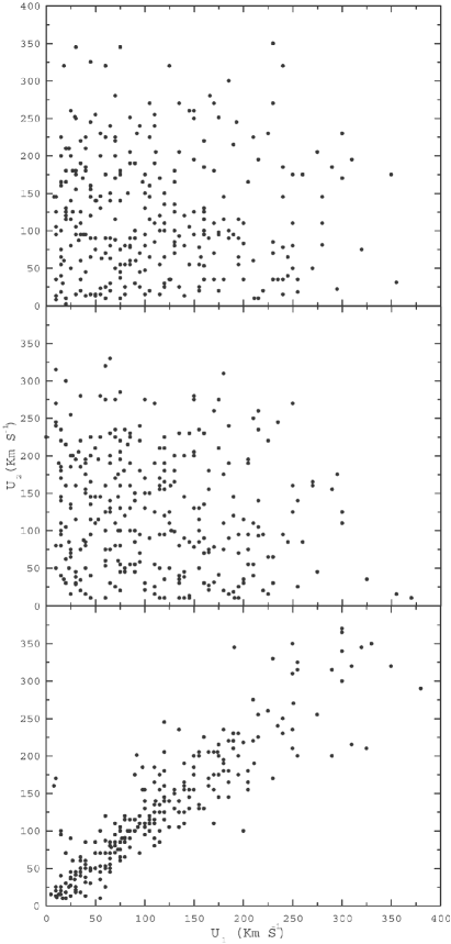
Figure 1: illustration of the projected rotational velocities of one component against the other for the samples AB (top), ABR (mid), and RB (bottom).

0.4 Analysis

0.4.1 Bivariate distribution, Marginal distribution, and Linear regression

We prepare a table for each of the three samples, AB, ABR and RB: it gives the discrete bivariate distribution of the samples. We give also the regression of the mean velocity of one component on the other one, as defined by equation (1).

$$\overline{u}_{1}\left({u_{2}\left(j\right)}\right)=\frac{\sum\limits_{i=1}^{7}{u_{1}\left(i\right)F\left({u_{1}\left(i\right),u_{2}\left(j\right)}\right)}}{\sum\limits_{i=1}^{7}{F\left({u_{1}\left(i\right),u_{2}\left(j\right)}\right)}}\$$ (1)

Here $u_{1}=v_{1}sini_{1}$ is the projected rotational velocity of the component, and $F(u_{1},u_{2})$ is the bivariate distribution.

For better illustration we show the regression of projected rotational velocity distribution of one component on the other one for each of the three samples. The $F(u_{1},u_{2})$ distributions for the samples AB, ABR, and RB are given in table 1. The marginal distribution and the regression lines are also shown. The latter are plotted in Fig.2. For the ease of comparing the current results with previous ones, the velocity range has been divided into subintervals of 50 km s^-1.

10 $\begin{array}[]{cc}&u1\\ u2&\\ \end{array}$ 0-50 50-100 100-150 150-200 200-250 250-300 300-350 $\phi_{2}(u_{2})$ $\bar{u}_{1}(u_{2})$ 0-50 563 525 406 351 200 90 51 0.22 115 50-100 617 575 446 388 221 99 58 0.24 116 100-150 451 420 324 282 161 73 42 0.18 115 150-200 433 404 313 271 155 70 41 0.17 116 200-250 276 260 200 174 99 45 26 0.11 116 250-300 122 115 88 77 44 20 12 0.05 116 300-350 104 99 76 67 39 17 10 0.04 117 $\phi_{1}(u_{1})$ 0.26 0.24 0.19 0.16 0.09 0.04 0.02 $\bar{u}_{2}(u_{1})$ 125 126 126 126 126 126 127 0-50 576 496 385 356 205 105 0 0.21 112 50-100 657 627 466 412 215 94 0 0.25 108 100-150 452 447 331 277 141 56 22 0.17 110 150-200 465 454 335 276 143 57 22 0.18 109 200-250 290 264 201 172 96 45 18 0.11 112 250-300 115 99 80 65 37 19 7 0.04 112 300-350 115 88 74 66 43 25 10 0.04 119 $\phi_{1}(u_{1})$ 0.27 0.25 0.19 0.16 0.09 0.04 0.01 $\bar{u}_{2}(u_{1})$ 126 125 126 124 125 125 201 0-50 1901 198 20 0 0 0 0 0.21 31 50-100 614 1564 158 40 10 0 0 0.24 68 100-150 40 515 1000 158 0 0 0 0.17 112 150-200 69 79 574 752 158 59 10 0.17 156 200-250 10 50 99 535 347 50 40 0.11 190 250-300 0 0 30 59 228 119 30 0.05 231 300-350 0 10 10 50 129 198 89 0.05 254 $\phi_{1}(u_{1})$ 0.26 0.24 0.19 0.16 0.09 0.04 0.02 $\bar{u}_{2}(u_{1})$ 43 89 144 193 242 278 284 a$u_{1}$ and $u_{2}$ are given in units of $10^{-4}$ km s^-1.

Table 1: Discrete distribution function ${F(y_{1},y_{2})}$ of the projected rotational velocities of the components of sample AB (top), ABR(middle), and RB(bottom).

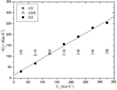
Figure 2: Regression of the mean rotational velocities of one component (ordinate) as a function of the rotational velocity interval of the second component (abscissa) for samples AB (top), ABR (mid), and RB (bottom).

No significant differences between the main diagonal and other components of the table are evident for the samples AB and ABR. But the set RB shows a distinct difference between the main diagonal and other elements of the table, indicating the presence of correlation of projected spins in real binaries.

0.4.2 Modified Convolution Test

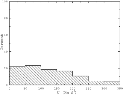
Figure 3: Projected rotational velocity distribution of all components grouped into intervals of 50 km s^-1.

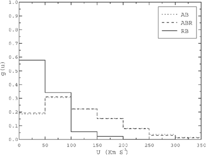
Figure 4: Modified convolution of rotational velocities.

Further illustration of the correlation between the rotational velocity distribution in real binary systems, and not in artificial ones, is to evaluate the modified convolution of the distribution functions. To validate the result, we first look at the single star velocity distribution, as shown in Fig. 3. The distribution is rather flat and does not indicate a strong maximum at any specific speed. Our modified convolution is essentially $g(u)=\int{P(v-u|v)dv}$, which in the discrete case is:

$$g(u)=\sum\limits_{v}{F(v-u,v)}$$ (2)

As expected from the flatness of the distribution in Fig. 3., the convolution of artificial binary systems do not indicate a concentrated, sharp peak. However, for real binaries, there is a rather sharp peak present. It means that probability for the projected rotational velocity difference to be smaller than 50 km s^-1 is almost 60%. The probability for the difference to be smaller than 100 km s^-1 is more than 90%(!) in real binaries.

0.5 Conclusions

We examined three samples of binaries. For each of the samples we applied identical tests, to render significant comparisons between artificial binaries and real ones.

As expected, correlation in artificial systems (Set AB and ABR) is insignificant. This is indicated by the miniscule slope of the regression lines. However, correlation for the Binary set RB (Real Binaries) is clearly evident (u₁=.856u₂+32). One can describe our results roughly as follows:

$$v_{1}\ sini_{1}\cong v_{2}\ sini_{2}\$$ (3)

This relation can be understood either as:

1. $v_{1}\ll\ v_{2}$ while $sini_{1}\gg\ sini_{2}$,

   or

2. $v_{1}\simeq\ v_{2}$ as well as $sini_{1}\simeq\ sini_{2}$.

Since we have used a sample containing 1010 systems, the probability of the first case to be real is extremely small. We rather accept the second explanation. We interpret this as meaning that:

1. Spin axes of members in binary systems are roughly parallel.

2. Rotational speeds are correlated.

There have been several investigations related to binary systems (Giuricin et al., 1984; Levato, 1976; Zhan, 1977; and Pan, 1997). These papers points out the importance of tidal interaction in close binary systems (especially the theory given by Zhan, 1966, 1970, 1975, 1977).

We suppose that only a small fraction of the sample RB contains close binary systems. Thus, we lack a general theory which can account for the empirical results demonstrated here.

References

- (1) Abt H. A., ApJ, 2001, 122, 2008
- (2) Giuricin G., Mardirossian F., & Mezzetti M., AA, 1984, 131, 152
- (3) Giuricin G., Mardirossian F., & Mezzetti M., AA, 1984, 135, 393
- (4) Glebocki R., Gnacinski P., & Stawikowski A., Acta Astron., 2000, 50, 509
- (5) Levato, H., AA, 1974, 35, 259
- (6) Levato, H., ApJ, 1976, 203, 680
- (7) Pan K., AA, 1997, 321, 202
- (8) Slettebak, A., 1963, ApJ, 138, 118
- (9) Steinitz, R., & Pyper, D. M., 1970, Stellar Rotation, ed. A. Slettebak
- (10) Zahn J. P., Ann. A, 1966, 29, 313, 489, 685
- (11) Zahn J. P., AA, 1970, 4, 452
- (12) Zahn J. P., AA, 1975, 41, 329
- (13) Zahn J. P., AA, 1977, 57, 383