Far-ultraviolet Spectroscopy of Magnetic Cataclysmic Variables

Abstract

We have obtained HST/STIS data for a total of eleven polars as part of a program aimed to compile a homogeneous database of high-quality far-ultraviolet (FUV) spectra for a large number of cataclysmic variables (CVs). Of the eleven polars, eight were found in a state of low accretion activity (V347 Pav, VV Pup, V834 Cen, BL Hyi, MR Ser, ST LMi, RX J1554.2+2721 and V895 Cen) and three in a state of high activity (CD Ind, AN UMa and UW Pic). The STIS spectra of the low-state polars unambiguously reveal the photospheric emission of their white dwarf (WD) primaries. We have used pure hydrogen WD models to fit the FUV spectra of the low-state systems (except RX J1554.2+2721, which is a high-field polar) in order to measure the WD effective temperatures. In all cases, the fits could be improved by adding a second component, which is presumably due to residual accretion onto the magnetic pole of the WD. The WD temperatures obtained range from 10 800 K to 14 200 K for $\log g=8.0$. Our analysis more than doubles the number of polars with accurate WD effective temperatures. Comparing the WD temperatures of polars to those of non-magnetic CVs, we find that at any given orbital period the WDs in polars are colder than those in non-magnetic CVs. The temperatures of polars below the period gap are consistent with gravitational radiation as the only active angular momentum loss mechanism. The differences in WD effective temperatures between polars and non-magnetic CVs are significantly larger above the period gap, suggesting that magnetic braking in polars might be reduced by the strong field of the primary. We derive distance estimates to the low-state systems from the flux scaling factors of our WD model fits. Combining these distance measurements with those from the literature, we establish a lower limit on the space density of polars of $1.3\times 10^{-6}\,\rm pc^{-3}$.

1 Introduction

Polars, also called AM Her stars, are cataclysmic variables (CVs) containing a white dwarf (WD) with a strong magnetic field ($\rm B\geq 10\,MG$) and a Roche lobe filling late type star (the secondary) that is losing mass to the WD through the inner Lagrangian point ($L_{1}$). For the typical $B\sim 10-80$ MG fields in polars, the material travels on a ballistic trajectory from $L_{1}$ to a point where the magnetic pressure exceeds the ram pressure of the accretion stream. At that point, the material is captured by the field and falls along the field lines to the magnetic pole or poles of the WD. A disk does not form because the material is captured before it reaches the stream circularization radius. The strong magnetic interaction between the WD and the donor star also results in the synchronization of the WD with the orbital period of the system. Due to the absence of a disk, polars do not show the outbursts characteristic of dwarf novae. Instead, they undergo deep low states on irregular timescales of months to years, up to three magnitudes fainter than their bright (high) states, during which the WD accretes at an extremely low rate. Since there is no disk to buffer the material before it reaches the WD, variations in accretion rate onto the WD directly reflect changes in the mass loss rate of the secondary (possibly due to star spots covering $L_{1}$; Hessman et al., 2000). Even though mass transfer via Roche lobe overflow may cease during a low state, the WD might still accrete some material from the donor star wind, as occurs in post common envelope binaries (see e.g.  O’Donoghue et al., 2003). The sources of ultraviolet (UV) emission that dominate in the high state - a hot polar cap near the footpoint of the accretion column, contributing most in the far-UV (FUV), and the X-ray illuminated accretion stream - greatly weaken or completely disappear during low-states. In this situation, the WD photosphere is the main source of FUV-radiation (e.g Gänsicke et al., 1995; Stockman et al., 1994; Gänsicke, 1998a; Gänsicke et al., 2000; Rosen et al., 2001; Schwope et al., 2002) and the effective temperature of the WD can be directly measured.

With typical effective temperatures in the range $10\,000-50\,000$ K, the best-suited wavelength range to observe CV WDs is in the region from $1500-3000$Å. As a consequence, much of the efforts on studying CV WDs were directed to the UV regime. The first measurements of WD effective temperatures in CVs were carried out with the International Ultraviolet Explorer (IUE) two decades ago (Mateo & Szkody, 1984; Panek & Holm, 1984). As a result of the IUE observations, Sion (1985, 1991) recognized that WDs in CVs were hotter than field WDs of comparable age, and suggested that compressional heating by the accreted material could account for this fact. More recently, Townsley & Bildsten (2002b, 2003, 2004) have carried out detailed studies of the long term effects of accretion on the thermal structure of the core and the envelope, including low-level nuclear burning, and have determined a relationship between the long-term average accretion rate and the photospheric temperature of the WD. This makes the measurement of CV WD temperatures an extremely important issue, since the secular mean of the mass accretion rates is key to understanding the evolutionary history of CVs.

A total of 23 polars were observed with IUE during its long and successful history, and these observations allowed a number of important insights into the accretion process of magnetic CVs (see e.g.  de Martino, 1998, for a review). Only a handful of these systems were bright enough to obtain estimates of their WD temperatures (e.g.  Heise & Verbunt, 1988; Gänsicke et al., 1995, 2000), the vast majority of polars were too faint for IUE to obtain UV spectroscopy of their WDs during low states. The larger aperture of the Hubble Space Telescope (HST) allowed observations of fainter polars using the Faint Object Spectrograph (FOS) and the Goddard High Resolution Spectrograph (GHRS), but the number of different polars (and CVs in general) measured remained quite small (Stockman et al., 1994; de Martino et al., 1998; Rosen et al., 2001; Schwope et al., 2002). To address this problem, we undertook an HST snapshot survey with the goal of obtaining reasonable high quality FUV spectra of a substantial sample of CVs of all subclasses (Gänsicke et al., 2003). Here we report on the observations of the eleven polars obtained as part of this survey.

2 Observations and Data Reduction

FUV spectroscopy of eleven polars was obtained with HST/STIS in Cycle 11 (Table 1). The data were obtained using the G140L grating and the $52\arcsec\times 0.2\arcsec$ aperture, providing a spectral resolution of $R\approx 1000$ over the wavelength range $1150-1710$ Å. Since the total time involved in a snapshot observation is short ($\sim 35$ min), we chose to make the observations in ACCUM mode in order to minimize the instrument overheads, resulting in exposure times of $\simeq 12-15$ min. As a result of this choice, each observation resulted in a single time averaged spectrum of each polar. For the analysis described here, all of the data were processed within IRAF using CALSTIS V2.13b. Figure 1 shows the STIS spectra of the eleven polars that were observed.

During target acquisition, HST points at the the nominal target coordinates and takes a $5\arcsec\times 5\arcsec$ CCD image with an exposure time of a few seconds. Subsequently, a small slew is performed that centers the target in the acquisition box, and a second CCD image is taken. The acquisition images for these observations were obtained using the $\mathrm{F28\times 50LP}$ long-pass filter, which has a central wavelength of 7228.5 Å and a full-width at half maximum (FWHM) of 2721.6 Å. We have made use of the STIS acquisition images to establish the (quasi-simultaneous) brightness of the systems at the time of the FUV observations. We computed instrumental magnitudes from the acquisition images by performing aperture photometry with the sextractor (Bertin & Arnouts, 1996). We then obtained from the HST archive a number of acquisition images of well-calibrated flux standards (GRW$+70^{\circ}$5824 and G191 B2B) to convert the instrumental magnitudes into $\mathrm{F28\times 50LP}$ magnitudes. Testing the method on a number of STIS observations of objects of known and constant magnitudes shows that the acquisition images can be used to determine the visual magnitude to typically $\pm 0.1$ mag. The response of the $\mathrm{F28\times 50LP}$ filter is closest to that of an $R$ filter, but extends further both into the blue and red.

Based on the appearance of the FUV spectra (Fig. 1) and the $\mathrm{F28\times 50LP}$ magnitudes (Table 1), three of the systems that we observed were found in a high state: CD Ind, AN UMa and UW Pic. Their FUV spectra are characterized by a nearly-flat continuum superimposed by strong emission lines of He, C, N, and Si. During the high state, the dominant FUV emission sources in polars are the heated polar cap (or hot spot) and the accretion stream. Line emission is the result of photoionization of the accretion stream by the high-energy photons from shocks in the accretion column and/or the impact regions of material on the WD surface. CD Ind, AN UMa and UW Pic exhibit similar emission line ratios of C IV $\lambda\lambda 1548,1551$, He II $\lambda 1640$, N V $\lambda\lambda 1239,1243$, Si IV $\lambda\lambda 1394,1403$, C III $\lambda 1176$, Si III $\lambda 1207$ and C II $\lambda 1333$ (see next section), the latter being the weakest in all three systems (Fig. 1). The Si III $\lambda\lambda 1295$–1303 multiplet is also present in CD Ind and to some extent in AN UMa but absent in the spectrum of UW Pic. The emission lines are highly asymmetric, consistent with their origin in the accretion stream, which has a large velocity gradient. The narrow ${\rm Ly\alpha}$ absorption (superposed on the broader emission) seen in the spectra of CD Ind and UW Pic is of interstellar origin.

Eight polars were observed in a state of very low accretion activity, as indicated by the weakness (V347 Pav, VV Pup, ST LMi and RXJ1554.2+2721,) or absence (V834 Cen, BL Hyi, MR Ser and V895 Cen) of emission lines (Fig. 1). All of the low state systems show the broad ${\rm Ly\alpha}$ absorption feature that is characteristic of a WD-dominated system. In addition, the $\mathrm{F28\times 50LP}$ magnitudes of these systems are consistent with the brightness level of previously observed low states (Table 1). In V895 Cen, the $\mathrm{F28\times 50LP}$ magnitude is close to the observed high-state V magnitude. However, in this long period polar the secondary star significantly contributes in the red also during the high state (Craig et al., 1996; Stobie et al., 1996; Howell et al., 1997). Consequently the high-to-low state variation in the $R$ band is low and the $\mathrm{F28\times 50LP}$ magnitude is only of limited use to determine the state of the system. Unfortunately, no $R$ low/high state magnitudes have been published for V895 Cen, except the USNO catalogue entry of $R=$15.9. Comparing this value to $\mathrm{F28\times 50LP}$=16.4 supports that the STIS observations were obtained during a low state of accretion. The fact that the WD is clearly visible in these systems allows us to obtain one of their fundamental system parameters, the WD temperature ($T_{\rm wd}$), as well as to estimate their distances.

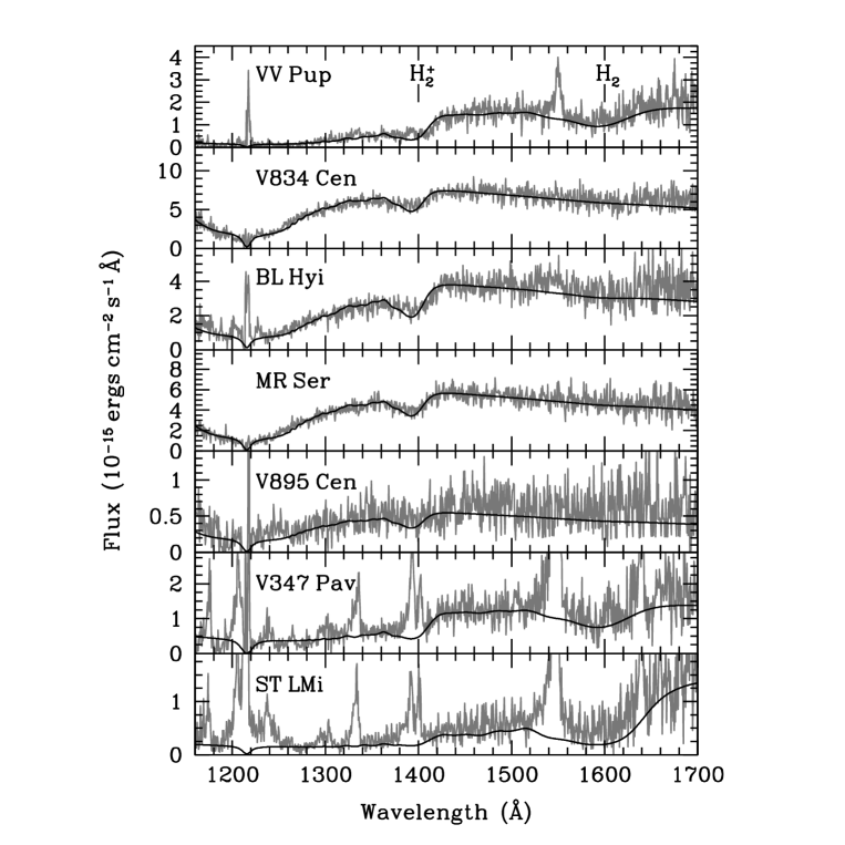
Figure 4: HST/STIS spectra (grey line) of the seven systems found in a low-state of accretion. Plotted over (black line) is the best 2-WD model for each of the systems. The parameter values for each of the models are given in Table 5.

A common feature in the FUV spectra of the low-state systems in Fig. 1 (see also Fig. 4), with the exception of RX J1554.2+2721 (RX J1554 for simplicity), is the presence of quasi-molecular hydrogen $\mathrm{H}^{+}_{2}$ at $\sim 1400$ Å. Also present in VV Pup, BL Hyi, V347 Pav and ST LMi is absorption by quasi-molecular hydrogen $\mathrm{H_{2}}$ at $\sim 1600$Å. The nature of both quasi-molecular features, first identified in WDs by Koester et al. (1985) and Nelan & Wegner (1985), is attributed to perturbations of the potential energy between the ground and first excited state of a neutral hydrogen atom caused by a proton or by another neutral hydrogen atom. In both cases the perturbation results in a shift of the energy of the emitted/absorbed photon, producing $\rm H^{+}_{2}$ ${\rm Ly\alpha}$ absorption at $\sim 1400$ Å in the case of a perturbing proton, and producing $\rm H_{2}$ ${\rm Ly\alpha}$ absorption at $\sim 1600$ Å in the case of a perturbing neutral hydrogen atom. The strength of both features depends strongly on the temperature of the hydrogen plasma (i.e. the WD atmosphere): the $1400$ Å feature is present for $\mbox{$T_{\rm wd}$}\lesssim 20\,000$ K and the 1600 Å feature is only visible for $\mbox{$T_{\rm wd}$}\lesssim 13\,500$ K.

In contrast to the spectra of quiescent dwarf novae, the low state spectra of polars show no metal absorption lines. In fact, not a single IUE or HST observations of any polar shows metal absorption line strengths anywhere close to those observe in non-magnetic systems (see e.g.  Gänsicke et al., 1995). This is in agreement with the idea that metal rich accreted material is coupled to the magnetic field lines and sinks deep into the WD atmosphere. Not until the gas pressure within the atmosphere exceeds the magnetic pressure can the material break free and spread laterally, and this occurs at large optical depths (Beuermann & Gänsicke, 2003).

An interesting feature in the low-state STIS spectrum of BL Hyi is that it shows two emission lines centered on ${\rm Ly\alpha}$. We believe that this is due to Zeeman splitting of ${\rm Ly\alpha}$ and in Fig.1 we identify the emission lines as the ${\rm Ly\alpha}$ Zeeman $\pi$, $\sigma^{+}$ and $\sigma^{-}$ components. This is only the second time in which Zeeman splitting has been observed in an emission line (EF Eri; Seifert et al., 1987) and the first time it has been observed in ${\rm Ly\alpha}$. We defer further discussion of this system to Sec. 4.4.

The FUV spectrum of RX J1554 reveals a very unusual broad absorption line centered on $\sim 1280$ Å (Fig. 1). We identify this feature as the ${\rm Ly\alpha}$ Zeeman $\sigma^{+}$ component, split in a field of $B>100$ MG, analogous to that observed in the FUV spectrum of AR UMa, whose magnetic field strength is $B=230\rm\,MG$ (the highest magnetic field among CVs; Schmidt et al., 1996; Gänsicke et al., 2001a). A full account of RX J1554 is given by Gänsicke et al. (2004). Due to its high field strength, the temperature determination of the WD in RX J1554 is subject to large systematic uncertainties, and we will not further discuss the properties of this object in the context of the present paper.

3 Polars observed in a high state

In previous HST/STIS and IUE studies of the prototype polar AM Her, Gänsicke et al. (1995, 1998) have shown that during high states a large heated pole cap dominates the FUV continuum emission at wavelengths $\lesssim 1500$ Å. During the high state, the emission from the polar cap in AM Her, even though arising from a high-gravity photosphere, showed only a very shallow broad ${\rm Ly\alpha}$ absorption line. Using a semi-empirical model, Gänsicke et al. (1998) showed that irradiation by thermal bremsstrahlung and/or cyclotron radiation from the accretion column is likely to flatten out the temperature gradient in the WD atmosphere around the accretion column, resulting in a significantly decreased depth of the ${\rm Ly\alpha}$ absorption compared to an undisturbed WD atmosphere. There is no evidence for broad ${\rm Ly\alpha}$ absorption ($\simeq 100$ Å) in any of the three high-state systems (see Fig.2). In contrast, in CD Ind (and, less clearly, in UW Pic) a broad emission bump centered on ${\rm Ly\alpha}$ is observed. Such feature could arise if irradiation results in a temperature inversion in the WD atmosphere at a significant depth, where pressure (Stark) broadening is sufficient to affect the ${\rm Ly\alpha}$ profile over $\simeq 100$ Å. Full phase-resolved FUV spectroscopy would be necessary to assess this hypothesis.

The line properties of the high-state systems in Fig. 2 are summarized in Table 2. A single Gaussian was fitted to each of the lines in the normalized spectrum with the exception of the Si IV $\lambda\lambda 1394,1403$ doublet where a double Gaussian fit was carried out. We also computed the following line flux ratios: He II/C IV, Si IV/C IV and N V/C IV (see Table 3), which fall within the normal range observed in CVs (Mauche et al., 1997; Gänsicke et al., 2003). As observed by Mauche et al. (1997) from a small sample of polars, there is a tendency within these three systems of exhibiting increasing N V/C IV ratios with increasing Si IV/C IV, with the He II/C IV ratio remaining approximately constant.

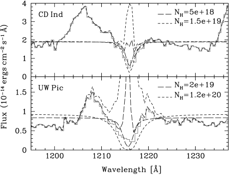
Figure 3: Interstellar ${\rm Ly\alpha}$ absorption of the spectra of CD Ind (top panel) and UW Pic (bottom panel) plotted in grey. Dash lines are the artificial ${\rm Ly\alpha}$ profile for different values of $N_{\rm H}$ as well as the corresponding corrected spectra.

In CD Ind and UW Pic, a narrow ${\rm Ly\alpha}$ absorption line is detected, which is of interstellar origin and allows a determination of the column densities of neutral hydrogen along the line of sight to these objects. We modeled the ${\rm Ly\alpha}$ interstellar absorption profile with a Lorentzian profile (Bohlin, 1975) with the neutral hydrogen column density ($N_{\rm H}$) and the profile broadening as free parameters. The broadening parameter used for both systems was the STIS resolution (i.e. $\simeq$1.2Å). The broadening produced by the turbulent velocity of the interstellar medium is so small compared with the instrumental resolution that it can be neglected here. In the case of CD Ind, the resulting neutral column density is $(1.0\pm{0.5})\times 10^{19}\,\mathrm{cm^{-2}}$, well within the upper limit $\rm 4.5\times 10^{20}\,cm^{-2}$ determined from radio 21 cm data (i.e. value of the entire content of $N_{\rm H}$ along the line of sight of CD Ind; Dickey & Lockman 1990). Our estimate is consistent with and should be more accurate than the more model dependent value of $(0.4\pm 1.0)\times 10^{20}\,\mathrm{cm^{-2}}$ obtained by Schwope et al. (1997) from ROSAT observations. The top panel of Fig. 3 shows the computed interstellar ${\rm Ly\alpha}$ profiles for values of $\mbox{$N_{\rm H}$}=0.5\times 10^{19}\,\mathrm{cm^{-2}}$ and $\mbox{$N_{\rm H}$}=1.5\times 10^{19}\,\mathrm{cm^{-2}}$. Also shown is the FUV spectrum of CD Ind corrected for the two respective values of $N_{\rm H}$. For $\mbox{$N_{\rm H}$}>1.5\times 10^{19}\,\mathrm{cm^{-2}}$, the correction produces an unrealistically strong ${\rm Ly\alpha}$ emission line. Due to clear signs of ${\rm Ly\alpha}$ emission in the spectrum of UW Pic, red-shifted due to the orbital motion at the time of the STIS observations, fitting the interstellar ${\rm Ly\alpha}$ absorption is prone to some systematic uncertainties, and we estimate a lower limit to be $\mbox{$N_{\rm H}$}>2\times 10^{19}\,\mathrm{cm^{-2}}$. This lower limit is consistent with the value of $\mbox{$N_{\rm H}$}=1.2\times 10^{20}\,\mathrm{cm^{-2}}$ reported by Reinsch et al. (1994), which they derived from the analysis of ROSAT observations. Plotted on the bottom panel of Fig. 3 is the ${\rm Ly\alpha}$ profile for values of $\mbox{$N_{\rm H}$}=2.0\times 10^{19}\,\mathrm{cm^{-2}}$ together with $\mbox{$N_{\rm H}$}=1.2\times 10^{20}\,\mathrm{cm^{-2}}$ of Reinsch et al. (1994). As in the case of CD Ind, we corrected the observed spectrum for the respective interstellar ${\rm Ly\alpha}$ absorption profiles to be able to judge the best models. Certainly, the value for $N_{\rm H}$ cannot be greater than $1.2\times 10^{20}\,\mathrm{cm^{-2}}$, as this would imply a broader ${\rm Ly\alpha}$ absorption profile than it is observed. Therefore, we believe that the real value for $N_{\rm H}$ along the line of sight of UW Pic is clearly in between the two values plotted on Fig. 3, which are well within the upper limit $4.5\times 10^{20}\rm\,cm^{-2}$, estimated from radio 21 cm data (Dickey & Lockman, 1990).

4 Polars observed in a low state

Previous analysis of IUE and HST/FOS observations of AM Her (Gänsicke et al., 1995; Silber et al., 1996), DP Leo (Stockman et al., 1994; Schwope et al., 2002), and HU Aqr (Gänsicke, 1998a) have demonstrated that the FUV flux of these polars during a low state can be interpreted in terms of photospheric emission from the WD with two different temperature regions: a small accretion-heated region – the polar cap (or hot spot) –  and a larger area with a relatively low temperature representing the “unheated” WD photosphere. The main focus of our analysis here is to determine the temperatures of the WDs in seven of the polars observed with STIS in a state of low accretion activity (Table 1). The approach we have adopted is to fit the STIS data of each of the systems with model spectra consisting of (a) a single WD; (b) a WD and a power-law; and (c) a two-component WD model. The two-component WD model is intended to represent the region of the WD unaffected by accretion and the hot spot at the base of the accretion column. We believe this model is the most physically reasonable of the three approaches. However, the other two models are important to assess the need for a second component and assess whether we have statistically significant evidence for our specific hot spot temperatures.

4.1 WD model spectra and fitting routine

We created a grid of local thermodynamic equilibrium (LTE), pure hydrogen (DA) WD non-magnetic model spectra with temperatures ranging from 8000 K to 60 000 K, using the codes TLUSTY/ SYNSPEC (Hubeny, 1988; Hubeny & Lanz, 1995). The spectra were smoothed to the resolution of the STIS. No additional broadening is expected since the WDs in polars are phase-locked to the secondary and therefore rotational effects are very small. We computed model spectra for three values of the surface gravity, $\log g=$ 7.5, 8.0, and 8.5. In this way we cover WD masses of $\mbox{$M_{\rm wd}$}\simeq 0.33-0.90\,\mbox{$M_{\odot}$}$, which is the typical range of WD masses found in CVs.

The assumption of LTE is well-justified for the temperature range considered here. In contrast to non-magnetic CVs, the FUV spectra of polars show no noticeable metal absorption lines, and therefore the use of pure-hydrogen models is appropriate. The field strengths of the systems studied here (Table 1) are too low to cause significant changes in the ${\rm Ly\alpha}$ profile due to Zeeman-splitting. The spectrum of BL Hyi ($B=23$ MG; Schwope & Beuermann, 1990; Ferrario et al., 1996) in Fig. 1 shows Zeeman-splitting of ${\rm Ly\alpha}$ in emission whose components are well within the broad ${\rm Ly\alpha}$ absorption originating in the WD atmosphere. This illustrates that fields of this magnitude do not modify the ${\rm Ly\alpha}$ profile significantly. Therefore, despite the fact that we have not attempted to create spectra for magnetic DAs, we believe the temperatures are reliable. In addition, all the polars studied here are cold enough to show strong quasi-molecular $\rm H_{2}^{+}$, and in some cases quasi-molecular $\rm H_{2}$ absorption lines (see Fig. 4). The dominant uncertainty in our approach is due to the unknown masses of the WDs. In fact, $T_{\rm wd}$ and $M_{\rm wd}$ (or $\log g$) are correlated as the width of ${\rm Ly\alpha}$ increases with higher WD mass as well as with lower effective temperatures. We explore below quantitatively the dependence of the best-fit $T_{\rm wd}$ on $\log g$.

Our fitting routine permits the use of single or multi-component spectral models, and uses $\chi^{2}$ minimization as best-fit criterion. In carrying out the fits, we masked the emission lines in the spectra of VV Pup, BL Hyi, V895 Cen, V347 Pav and ST LMi; the other low-state spectra were emission line-free. Free parameters in the fit are the temperature (or power-law index) and the scaling factor of each component. The scaling factor between the model spectra and the observed data is defined as

$$\frac{f}{H}=4\pi\frac{\mbox{$R_{\rm wd}$}^{2}}{d^{2}},$$ (1)

where $f$ and $H$ are the “de-reddened” flux and the Eddington flux of the model, respectively, and $R_{\rm wd}$ and $d$ are the WD radius and the distance to the system. We have assumed negligible reddening for all seven systems (consistent with the absence of detectable reddening in the IUE spectra of V834 Cen, BL Hyi, VV Pup and MR Ser; La Dous, 1991). However, in order to test the effect of reddening ($E_{(B-V)}$) on the fits we repeated the fits assuming $E_{(B-V)}=0.05$, which can be considered a conservative upper limit for these relatively nearby high-galactic latitude systems. The WD temperatures did not change by more than $\simeq 200$ K. The scale factors increased by a factor of $\simeq 1.5$ compared with $E_{(B-V)}=0$ because the de-reddened flux is higher. This translates into a decrease of $\simeq 20\%$ on the derived distance estimates, which is within the error introduced by the uncertainty of the WD mass (see Sect. 4.3).

4.2 WD effective temperatures

As outlined above, our first approach was to fit the STIS spectra of the seven low-state polars using a single temperature WD model. The results from this exercise are reported in Table 5. The uncertainties in the derived temperatures and scaling factors are obtained from three separate fits using $\log g=7.5$, 8.0, and 8.5 models, and reflect the fact that the WD masses of these systems are unknown. It is apparent that the uncertainty in the WD masses translates into only a relatively small uncertainty in the derived values for $T_{\rm wd}$. The $\chi^{2}_{\nu}$ values obtained from the three fits (i.e. for $\log g=$7.5, 8.0 and 8.5 respectively) to each of the spectra are essentially the same. This underlines the fact that it is not possible to independently determine $T_{\rm wd}$ and $M_{\rm wd}$ from the STIS data alone.

Guided by the experience of Stockman et al. (1994), Gänsicke et al. (1995), Gänsicke (1998a) and Schwope et al. (2002), as well as by the relatively high values of $\chi^{2}_{\nu}$ for a number of systems (Table 5) we fitted the STIS spectra of the seven polars with the two-component models introduced above: a WD plus a power-law or two WD components with different temperatures. In all cases the two-component model improves the fit, most noticeably for V834 Cen, BL Hyi and MR Ser. However, based on $\chi^{2}_{\nu}$, we are unable to chose between models that use a power-law or WD spectrum as the second component. Furthermore, we found that the temperature of the second WD component, typically in the range 30 000 K$-$70 000 K, was poorly constrained by the fits. This is not very surprising since in our spectral range, the slope of the hotter WD continuum is close to the Rayleigh-Jeans limit and the ${\rm Ly\alpha}$ profile is weak and relatively narrow. Varying the temperature of the hot component had little effect on the resulting temperature and scaling factor for the cold WD component. Our conclusion is that while a second component improves the fits, we cannot on the basis of statistics (a) distinguish between power law fits and WD models for the second component, or (b) accurately determine the temperature and fractional size of the second component from the two WD fits.

We therefore decided to report the fits using two WD components with the second component fixed at 50 000 K, comparable to the “hot spot” temperature of DP Leo and AM Her derived by Stockman et al. (1994) and Gänsicke et al. (1998) from phase resolved HST data. As for the single WD model approach, we fitted the STIS spectra for three values of $\log g=$ 7.5, 8.0 and 8.5. These results are listed in Table 5, with the errors reflecting the uncertainty in the masses of the WDs. In all cases the optical flux of the best two temperature fit model to each of the FUV spectra is consistent with the simultaneous optical flux obtained from the HST/STIS acquisition image. The ratio of the scale factors for a given distance and mass of the two temperature components (Table 5; $F[\%]=N_{2}/N_{1}\times 100$) gives an idea of the hot component contribution to our observations. This value needs to be interpreted with caution as due to the nature of the observations (snapshots which only cover a small portion of the orbital cycle) we are unable to properly quantify the true hot spot surface area with respect to the entire WD. Overall, the effective temperatures of the WDs did not change by large amounts compared to the single WD fits, but by analogy to the few polars for which phase-resolved low-state FUV observations exist, we believe that the WD temperatures determined from the two-component model are preferable.

4.3 Distances

Even though accurate distances to a few CVs have recently been determined directly through ground and space based parallax programs (Harrison et al., 2000; Thorstensen, 2003; Beuermann et al., 2003, 2004), the bulk of all available distance estimates is still based either on the absolute magnitude in outburst-orbital period relationship found by Warner (1987) (only in the case of dwarf novae), or on red/infrared observations of the donor stars in these systems. The latter technique is based primarily on the quasi-independent relation between surface brightness of cool stars in the $K$-band and their temperature (or luminosity) empirically found by Bailey (1981), and later refined by Ramseyer (1994). The most crucial assumption of this method is that the observed $K$-band magnitude is entirely due to emission from the secondary. Whereas in dwarf novae the outer (cooler) regions of accretion disks may contribute to the observed red/infrared flux the main source of contamination in polars is cyclotron emission. Hence, the $K$-band magnitude method is prone to underestimate the distances. A significant improvement of this method is achieved if the secondary can be detected spectroscopically; Beuermann & Weichhold (1999) presented a calibration of the surface brightness in the TiO absorption bands prominent in M-dwarfs found in short-period CVs, and conclude that with the appropriate data, distance estimates with an accuracy of $10\%$ can be obtained.

Here we make use of an independent method to estimate the distances of the polars observed in the low state, based on the surface brightness of the primaries in these systems through the normalization factor defined in Eqn. 1. To make use of this relation, we need to assume a mass-radius relation to convert the WD mass/$\log g$ into a stellar radius. For the low temperatures of the WDs considered here, the Hamada–Salpeter mass-radius relation (Hamada & Salpeter, 1961) is accurate enough. Obviously, the unknown WD mass is the largest systematic uncertainty in these estimates. Our WD model fits primarily reflect the shape of ${\rm Ly\alpha}$. At a given temperature, the ${\rm Ly\alpha}$ profile increases in width as the mass increases. At a given mass, the ${\rm Ly\alpha}$ profile decreases in width as the temperature increases. The physical reasons for these dependencies are as follows: A higher WD mass (higher $\log g$) implies a higher density in the WD atmosphere, resulting in an increase in the width of ${\rm Ly\alpha}$ due to the stronger Stark broadening. A higher temperature results in a narrower ${\rm Ly\alpha}$ profile, as the number of neutral hydrogen atoms decreases with increasing $T_{\rm wd}$. The same observed ${\rm Ly\alpha}$ profile can hence be fit approximately well with a somewhat hotter high-mass WD or a somewhat colder low-mass WD. Furthermore, the surface area of the WD is $\propto\mbox{$R_{\rm wd}$}^{2}$, and $R_{\rm wd}$ is anticorrelated with $M_{\rm wd}$. Combining all effects, we find that the systematic uncertainty in the distance is $\pm 13-23$ % for WD masses in the range $\mbox{$M_{\rm wd}$}=0.33-0.90$ $M_{\odot}$ (see Table 6). Using the WD as an independent distance estimator is not only useful to confirm distance measurements based on Bailey (1981)’s method (see e.g. Gänsicke et al. 1999; Araujo-Betancor et al. 2003; Hoard et al. 2004), but is the only feasible way to obtain distance estimates for systems in which the secondary is not detected, such as those likely to contain a brown dwarf donor (e.g. EF Eri: Beuermann et al. 2000, HS 2331+3909: Araujo-Betancor et al. 2004).

4.4 Individual systems

Here we discuss the results for the individual systems and compare our findings to previous studies.

VV Pup — Liebert et al. (1978) fitted a blackbody to an optical low state spectrum and estimated $\mbox{$T_{\rm wd}$}\simeq 9000$ K and 80 pc$<d<$150 pc. Bailey (1981) estimated $d\simeq 144$ pc based on the low-state $K$ band magnitude measured by Szkody & Capps (1980). VV Pup has been considered to host the coldest WD in a CV, however, our value of $T_{\rm wd}=11\,900$ K moves it to a significantly higher temperature. Blackbodies are relatively crude approximations to a WD spectra, and our STIS result should supersede the older estimate. Our estimate of the distance to VV Pup, $d=151\pm{28\atop 34}$ pc, agrees well within the errors with that obtained by Bailey (1981) using Bailey’s method, which in general gives lower limits and therefore we believe our value to be more robust.

V834 Cen — Maraschi et al. (1984)’s blackbody fit to simultaneous optical and IUE low-state spectra gave a $\mbox{$T_{\rm wd}$}=26\,500$ K WD within a distance of $d=50-200$ pc from the low state $R$ and $I$ magnitudes. They noted, however, that the WD interpretation of the UV continuum was somewhat ambiguous, as no broad ${\rm Ly\alpha}$ absorption was observed. Cropper (1990) applied Bailey’s method using $K=13.1$, as reported by Maraschi et al. (1984) during a high state. This value of $K$ is clearly an upper limit to the $K$-brightness of the secondary in V834 Cen and therefore the derived distance $d=86$ pc is an absolute lower limit. Further optical low-state spectroscopy and photometry was reported by Puchnarewicz et al. (1990), Schwope (1990) and Ferrario et al. (1992). Puchnarewicz et al. (1990) obtained $\mbox{$T_{\rm wd}$}=12\,000$ K from a blackbody fit to the optical low-state continuum and $d>70$ pc from the spectral signature of the companion. Interestingly, both Schwope (1990) and Ferrario et al. (1992) suggested a two-temperature model for the WD to fit the observations. Ferrario et al. (1992) showed a very smooth, quasisinusoidal blue light curve (their Fig. 5), which they interpreted as a hot spot of $T_{\rm spot}\simeq 50\,000$ K on a $\mbox{$T_{\rm wd}$}=15\,000-20\,000$ K WD with probably some cyclotron emission from a residual accretion column. Schwope (1990) modeled phase-resolved low state optical spectroscopy with a $\mbox{$T_{\rm wd}$}=15\,000$ K WD and a spot of 30 000 K. More recently, Gänsicke (1998b) reached the same conclusion as Ferrario et al. (1992) and Schwope (1990) about the need of two-temperature model to fit the observations of V834 Cen. They used IUE low state spectroscopy and find $\mbox{$T_{\rm wd}$}=15\,000$ K and $\mbox{$T_{\rm spot}$}=30\,000$ K. Our STIS value for the WD temperature of V834 Cen, $\mbox{$T_{\rm wd}$}=14\,300$ K, confirms the values reported by Schwope (1990) and Gänsicke (1998b), and our data clearly underline the need of a two-component model for V834 Cen in the low state. Our distance estimate, $d=144\pm{18\atop 23}$ pc appears realistic.

BL Hyi — As already mentioned in Sec. 2, the spectrum of BL Hyi exhibits Zeeman-splitting in the ${\rm Ly\alpha}$ emission (see Fig. 1). We measure the spacing between the central $\pi$ component and the $\sigma^{-}$ and $\sigma^{+}$ components of the ${\rm Ly\alpha}$ emission Zeeman-splitting to be $\Delta\lambda\sim 14$ Å. Using $\Delta\lambda=e\lambda^{2}B/4\pi m_{e}c^{2}$ (where $e$ is the electron charge and $m_{e}$ is its mass), or $B=1.45\Delta\lambda$ [MG] (for values of $\Delta\lambda$ in Å), we infer a field strength of $B\sim 20$ MG which is consistent with the value measured from cyclotron radiation and Zeeman absorption features ($B=23$ MG; Schwope & Beuermann, 1990; Ferrario et al., 1996). Considering that $B\propto 1/r^{3}$, the ${\rm Ly\alpha}$ emission line must arise therefore from emission regions very close to the white dwarf surface. A previous study of BL Hyi reported by Wickramasinghe et al. (1984) gave a value for the temperature of the WD of $\mbox{$T_{\rm wd}$}\simeq 20\,000$ K. In this case, the authors modeled low-state optical spectroscopy with simple magnetic WD models. Our estimate, $\mbox{$T_{\rm wd}$}=13\,300$ K, is significantly different from the above but agrees well with the estimate of Schwope et al. (1995), $\mbox{$T_{\rm wd}$}=13\,000$ K, obtained from modeling optical low-state spectroscopy of BL Hyi. Here the authors used a distance to the system of $d=132\pm 20$ pc, obtained via Bailey’s method. Our distance estimation $d=163\pm{18\atop 26}$ pc is consistent with the above.

MR Ser —Mukai & Charles (1986) fitted optical low-state spectroscopy with a composite model consisting of a blackbody plus M-dwarf template and found $\mbox{$T_{\rm wd}$}\simeq 9000$ K and $d=142$ pc. They mentioned, however, that the choice of $T_{\rm wd}$ was somewhat arbitrary, and they were mainly interested in the secondary star. Szkody et al. (1988) fitted IUE intermediate state data with WD models and found $\mbox{$T_{\rm wd}$}\simeq 20\,000\,K$. The absence of a ${\rm Ly\alpha}$ absorption line, characteristic of the WD photosphere, casts some doubt on the interpretation of the authors and the inferred value. Schwope et al. (1993) estimated $d=139\pm 13$ pc from the detection of the M5–M6 secondary star in optical low state spectroscopy which agrees well with our estimate, $d=160\pm{18\atop 26}$ pc. The same authors derived $\mbox{$T_{\rm wd}$}=8500-10\,000$ K from modeling the low state spectrum with WD spectra. The value obtained in the present work for the temperature of the WD, $T_{\rm wd}=14\,200$ K, is significantly higher than the previous estimates, but being based on the unambiguous signature of the WD in the FUV, we believe that our value is more accurate.

V895 Cen — Howell et al. (1997) estimated the distance to V895 Cen to be $d\simeq 250-295$ pc by using the absolute visual magnitude of the best main-sequence template fit to the optical spectrum and the measured $V$-magnitude. Our estimate of $d=511\pm{60\atop 81}$ pc puts V895 Cen significantly further away. As in the case of Bailey’s method, the method employed by Howell et al. (1997) gives lower limits for the distance since other sources within the system (apart from the secondary) might have contributed to the measured visual magnitude.

V347 Pav — Ramsay et al. (2004) modeled UV broadband fluxes obtained from the Optical Monitor (OM) on board of the XMM-Newton observatory to estimate $\mbox{$T_{\rm wd}$}<10\,200$ K and $d\simeq 40-50$ pc. Their observations were obtained during a high state, so the contribution of the accretion spot/stream to the UV flux was likely to have contaminated the emission from the WD, and broad-band fluxes were probably insufficient to permit a reliable determination of $T_{\rm wd}$. A WD temperature of $\mbox{$T_{\rm wd}$}=11\,800$ K at a distance $d=171\pm{33\atop 38}$ determined from our detailed STIS spectroscopy is certainly a more robust result. With Ramsay’s 2004 distance of $\simeq 40-50$ pc, V347 Pav would be one of the closest CVs known, and a ground-based parallax program would be worthwhile to test this hypothesis.

ST LMi —The first report on the temperature of the WD in ST LMi was made by Schmidt et al. (1983). In their paper they estimated $\mbox{$T_{\rm wd}$}=10\,000-25\,000$ K by comparing a low state optical spectrum of ST LMi to that of AM Her. Szkody et al. (1985) obtained a WD temperature of $\mbox{$T_{\rm wd}$}=13\,400\pm 2000$ K from blackbody fits to IUE low state spectra and optical/IR photometry. Bailey et al. (1985) estimated $d=136$ pc based on the faint-phase $K$ magnitude, and $\mbox{$T_{\rm wd}$}=12\,000-30\,000$ K from $U-B$ and $B-V$ colours. Mukai & Charles (1987) modeled optical low-state spectroscopy of ST LMi with a composite model consisting of a blackbody plus M-dwarf template (M5–M6). They found that any of the blackbody curves with temperature values within the range given by Bailey et al. (1985) (i.e. $\mbox{$T_{\rm wd}$}=12\,000-30\,000$ K) could equally well fit the observations. Our value of $\mbox{$T_{\rm wd}$}=10\,800$ K is the first unambiguous measurement of the WD temperature in ST LMi. Our distance estimate of $d=115\pm{21\atop 22}$ pc is consistent with Bailey’s 1985 value of $d=136$ pc.

5 Discussion

We have obtained HST/STIS FUV observations of a group of eleven polars, eight of which were found in a low accretion state. Thanks to the reduction of the mass transfer from the secondary, we were able to have a direct view at the WD allowing us to measure its temperature and to estimate the distances to the systems.

5.1 WD temperatures in the context of CV evolution

Measuring WD effective temperatures for seven polars from high-quality STIS data represents a substantial addition to the number of polars with well-determined WD temperatures. In order to discuss our results in the general context of CV WD temperatures, we have compiled in Table 7 a list of reliable CV WD temperature measurements. We only include values derived from WD model fits to FUV spectra which clearly show ${\rm Ly\alpha}$. The only exception is the short-period polar EF Eri, in which the WD is unambiguously detected at optical wavelength during a low state (Beuermann et al., 2000). We also exclude the WDs in the recently discovered polars, SDSSJ155331.12+551614.5 and SDSSJ132411.57+032050.5 (Szkody et al., 2004b), and in HS 0922+1333 (Reimers & Hagen, 2000) and WX LMi=HS 1023+3900 (Reimers et al., 1999), as so far there is no evidence that they have started Roche lobe overflow mass transfer.

Figure 5 shows the CV WD $T_{\rm wd}$ as a function of the orbital period for magnetic and non-magnetic CV WDs. Two important results are evident: (a) $T_{\rm wd}$ decreases toward shorter periods and (b) magnetic CVs show lower $T_{\rm wd}$ than non-magnetic CVs at any given period. The new results confirm suggestions by Sion (1991), who used the best available temperature information at the time: only two $T_{\rm wd}$ measurements were reliable in the sense that we have defined here (AM Her: Heise & Verbunt 1988 and V834 Cen: Schwope 1990).

The evolution of single WDs is driven by the cooling of their degenerate cores. Isolated WDs reach photospheric temperatures of $\mbox{$T_{\rm wd}$}\thickapprox 8000$ K after $\simeq 1$ Gyr and $\mbox{$T_{\rm wd}$}\thickapprox 4500-5000$ K after $\simeq 4$ Gyr (Salaris et al., 2000; Wood, 1995). CVs are believed to spend on average $\simeq 2$ Gyr as detached WD/main sequence binaries (Schreiber & Gänsicke, 2003). Once they start mass transfer, they evolve above the gap on time scales of a few 100 Myr, and below the gap on time scales of several Gyr (Kolb & Stehle, 1996). Comparing these time scales and the observed $T_{\rm wd}$ of CV WDs to the theory of WD cooling, it is evident that long term accretion-induced heating (with possibly some additional heating occurring during nova outbursts) is essential to compensate the secular core cooling.

According to the standard model of CV evolution (e.g. King, 1988, for a review), systems evolve to shorter orbital periods responding to angular momentum loss (AML) from the binary, with magnetic braking dominating in systems above the period gap and gravitational radiation in those below. While the standard theory explains the period gap by invoking a sudden decrease in magnetic braking (= decrease in accretion rate), it fails to explain a number of features that characterize the orbital period distribution of CVs (e.g. Kolb & Baraffe, 1999; Patterson, 1998; King et al., 2002). Several authors (Patterson, 1998; King et al., 2002, among others) have suggested an additional AML mechanism working below the period gap to resolve some of the discrepancies between the theory and the observations; notably the observed minimum period ($P_{\rm min}\sim 80$ min) compared to the predicted value ($P_{\rm min}\sim 65$ min), and the missing number of observed systems around $P_{\rm min}$, and below the 2 h orbital period in general, predicted by population synthesis models (Kolb & Baraffe, 1999). Townsley & Bildsten (2003) derived a relation between the mean mass accretion rate ($\langle\dot{M}\rangle$) and temperature of the WD so that for a given temperature $\langle\dot{M}\rangle$ can be estimated. Using their $\langle\dot{M}\rangle$-$T_{\rm wd}$ relations, Townsley & Bildsten (2003) concluded that the temperatures of non-magnetic CVs below the gap revealed mass accretion rates higher than those computed from gravitational radiation alone, providing an indirect evidence for an additional AML mechanism below the gap, which increases $\langle\dot{M}\rangle$.

Whereas the standard scenario predicts that magnetic and non-magnetic CVs will evolve in an indistinguishable way, Wickramasinghe & Wu (1994) and Li et al. (1994) have predicted that the strong magnetic fields in polars would result in the formation of closed field lines between the WD and the donor star. This will effectively reduce the number of the open field lines responsible for the drain of angular momentum from the system. Consequently, the mass transfer rates in polars are expected to be lower, and their evolution time scales longer compared to non-magnetic CVs.

Fig. 5 shows that for any given orbital period, WDs in magnetic CVs are colder than in non-magnetic CVs. Following the work of Townsley & Bildsten (2002a, 2003, 2004) this implies lower secular accretion rates in the strongly magnetic polars compared to the non-magnetic dwarf novae, and is consistent with the hypothesis of reduced magnetic braking in polars. The difference in WD effective temperature between magnetic and non-magnetic CVs is largest above the gap, but it is still significant below the gap. Assuming gravitational radiation as the only AML mechanism below the gap, there should be no differences between the WD effective temperatures of magnetic and non-magnetic CVs. Our finding of lower temperatures in polars compared to non-magnetic CVs also below the gap can be understood in a scenario where residual magnetic braking is important below the gap, but is reduced by the presence of a strong magnetic field on the WD.

While a difference in the long-term accretion rate between magnetic and non-magnetic CVs is the most likely mechanism to explain the differences in their WDs effective temperature, several other physical factors that could partially account for this effect need to be considered. As discussed by Townsley & Bildsten (2003) $T_{\rm wd}$ is a function of both, the secular mean accretion rate and the WD mass, as a larger mass implies a higher accretion luminosity per accreted gram of material. Considering this degeneracy in ($\dot{M},\mbox{$M_{\rm wd}$}$), the lower temperatures found in polars could be explained within a scenario where magnetic and non-magnetic CVs have the same mean accretion rates, but magnetic CVs have on average less massive WDs than non-magnetic CVs. While for single WDs the contrary is true, i.e. magnetic WDs are more massive than non-magnetic ones (Liebert et al., 2003), the situation is much less clear for CVs, as the CV WD mass values (with just a few exceptions) are subject to extreme systematic uncertainties.

Another effect to consider is the degree to which short term variations in the accretion history of the CVs being compared compromise the interpretation of $T_{\rm wd}$ as indicative of the long-term ($10^{5}$ yr) accretion rates that control the evolutionary history of CVs. Observations of some dwarf novae, e.g VW Hyi (Gänsicke & Beuermann, 1996) indicate that a WD returns to a quiescent state within 20 days of outburst, while the WD in WZ Sge had not fully cooled to its pre-outburst temperature 18 months after outburst (Long et al., 2003; Sion et al., 2003a). These differences likely reflect the different amounts of mass accreted during an outburst, much more in WZ Sge than in VW Hyi. The situation in polars is less understood, since essentially only one intensive study of interoutburst temperature measurements has been conducted. In AM Her, Gänsicke et al. (1995) have analyzed all available low-state IUE observations of AM Her, and found consistently $\mbox{$T_{\rm wd}$}\simeq 20\,000$ K, independent of the time passed since the previous high state. However, given the fact that the temperatures listed in Table 7 and shown in Fig. 5 were measured at random inter-outburst phases for the non-magnetic systems, and at random points during low states for the polars, some conspiracy appears to be necessary to explain the observed differences in $T_{\rm wd}$ by the effect of short-term heating/cooling. Obviously, given that the difference in $T_{\rm wd}$ between magnetics and non-magnetics is smallest in the region below the gap, this is where it is most difficult to rule out the effects of short term heating, and that only few systems with reliable $T_{\rm wd}$ are available above the gap, additional data would be desirable to improve the statistics of the temperature comparison.

5.2 Low-states versus high-states

In our survey of eleven polars, we have observed eight systems in a low-state of accretion (or $73\%$). Considering the relatively small number of systems, the percentage of those found in low state is in good agreement with the numbers found by Ramsay et al. (2004). In their study they observed a total of 37 polars with XMM-Newton of which 16 ($43\%$) were found in a low-state. They also re-examine a sample of the ROSAT All-Sky Survey data and found that 16 out of the 28 polars that were not discovered by ROSAT ($57\%$) were in a low-state. In their study the authors concluded that there was no evidence for a correlation between the orbital period and the occurrence of low states. That means that low states appear not to be connected with the evolution of the systems. Dedicated monitoring programs, aiming at mapping out the frequency of high and low states in polars, is needed in order to confirm this point and to search for any correlation with the WD magnetic field strength, which will improve our understanding of CV evolution.

5.3 Space density

Standard population models (e.g. de Kool, 1992; Kolb, 1993; Politano, 1996) typically give a galactic CV space density of up to $10^{-4}\,\mathrm{pc}^{-3}$. Assuming a scale height of $\sim 150$ pc above the galactic plane (Patterson, 1984; Thomas & Beuermann, 1998), a mid-plane density of $10^{-4}\,\mathrm{pc}^{-3}$ corresponds to $\simeq 680$ CVs within a distance of 150 pc (accounting for the exponential drop-off in density over one scale height decreases the effective volume by a factor $\simeq 2$) – compared to a few tens of known CVs with a confirmed $d\lesssim 150$ pc.

Within the error bars, we find six polars in our STIS sample that are within a distance of $\simeq 150$ pc: VV Pup, V834 Cen, BL Hyi, MR Ser, V347 Pav and ST LMi. Compiling the distance estimates for the other known polars from the literature, three additional systems are within a distance of 150 pc: AM Her ($d=79$ pc, Thorstensen 2003), EF Eri ($d\sim 150$ pc, Beuermann 2000; Thorstensen 2003), and AR UMa ($d\simeq 88$ pc, Remillard et al. 1994). Again assuming a scale height of 150 pc, the effective volume sampled is $6.81\times 10^{6}\mathrm{pc^{3}}$, which implies a space density of known polars of $1.3\times 10^{-6}\mathrm{pc^{-3}}$, compared to $\sim 4.4\times 10^{-6}\mathrm{pc^{-3}}$ of the known non-magnetic CVs with $d\lesssim 150$ pc.

Considering that the majority of polars have been discovered by their X-ray emission, that ROSAT has been the only all-sky-survey in this wavelength band, that polars spend on average $\simeq 50$% of their time in a low state, and that the local interstellar medium is inhomogeneous (Warwick et al., 1993) (which favors the discovery of systems in certain parts of the sky more than others), it is clear that the number derived above is an absolute lower limit on the space density of polars, and that the true value could be easily a factor $\simeq 2$ higher.

The total ratio of known magnetic/non-magnetic CVs is $\sim 22\%$ (if we only include confirmed AM Her stars and Intermediate polars; Downes et al., 2001) whereas it is $\sim 5\%$ for isolated WDs (Jordan, 1997; Wickramasinghe & Ferrario, 2000). If we assume that the fractional birthrate of magnetic to non-magnetic WDs should be similar for single WDs and those in CVs, then we must think of a mechanism that increases the fraction of magnetic CVs. The first and obvious mechanism are observational selection effects. Whereas it is true that ROSAT has been very efficient in finding magnetic CVs, the same is true for amateurs finding dwarf novae, and a quantitative comparison is difficult. However, spectroscopic optical surveys that are not biased towards X-ray emission but discover CVs on the base of their colours/emission lines consistently report the fraction of magnetic CVs in the range of $\simeq 10-20$ % Gänsicke et al. (2002); Marsh et al. (2002); Szkody et al. (2002a, 2003a, 2004a). An intrinsic mechanism of increasing the fraction of magnetic CVs is inherent to the discussion in Sect. 5.1: if strong magnetic fields on the WD indeed inhibit the efficiency of magnetic braking, then the evolution time scales of magnetic CVs are correspondingly longer, and the likelihood of discovering them at a given orbital period is increased with respect to non-magnetic CVs. A possible caveat to this line of reasoning is that the true fraction of isolated magnetic/non-magnetic WDs might be higher than suggested by previous studies. Liebert et al. (2003) have recently shown that the fraction of isolated magnetic/non-magnetic WDs of the local sample, which is considered as complete (to distances of 13 pc), is $11\%\pm 5\%$ for $B>2$ MG. This value is marginally consistent with the $\sim 5\%$ quoted by Jordan (1997) and Wickramasinghe & Ferrario (2000), but it underlines the need to understand observational selection effects.

6 Conclusions

We studied a group of eleven polars observed with HST/STIS as part of our snapshot program aimed at compiling a homogeneous data base of high-quality FUV spectra of CVs. Of the eleven AM Her systems under study here, we found eight in a low-state of accretion. One described in detail elsewhere (Gänsicke et al., 2004) is RXJ1554 with $B>100$ MG, the third high-field polar. A second is BL Hyi, for which we confirm a field of $\sim$20 MG from Zeeman splitting of ${\rm Ly\alpha}$ in emission, the first time ${\rm Ly\alpha}$ Zeeman splitting has been detected in emission. Thanks to the reduction of the mass accretion rate during low-states a direct study of the WD in these systems has been possible. We have derived their temperatures and distances to the system of the low-state polars in an uniform way by fitting their FUV spectra with WD models (with the exception of RX J1554, where the high field strength impedes an accurate $T_{\rm wd}$ determination). Our main conclusions are as follows:

1. The low-state spectra of VV Pup, V834 Cen, BL Hyi, MR Ser, 894 Cen, V347 Pav, and ST LMi can be well described with two-temperature models: a hot component with a small area (a hot polar cap) and a cold component which is ascribed to the ‘unheated’ photosphere of the WD. The seven polars analyzed have WD temperatures in the range 10 800 K–14 200 K.

2. Our analysis increases the sample of polars with well-determined $T_{\rm wd}$ from 6 to 13. Combining the $T_{\rm wd}$ obtained here with all reliable CV WD temperatures from the literature we find that the WDs in magnetic CVs are colder than those in non-magnetic CVs at any given orbital period.

3. Using the $\mbox{$T_{\rm wd}$}-\langle\dot{M}\rangle$ relation derived by Townsley & Bildsten (2003) we conclude that the temperatures of polars below the gap are consistent with those expected from gravitational radiation as the only mechanism removing angular momentum from the systems. This is in contrast with the result for non-magnetic CVs below the gap obtained by Townsley & Bildsten (2003), in which they found that an extra angular momentum loss mechanism is needed to explain the measured accretion rates. Above the gap, the WD temperatures in polars imply lower mean accretion rates than predicted by magnetic braking, which supports the hypothesis that a strong magnetic field on the primary will reduce the efficiency of magnetic braking.

4. The total ratio of known magnetic/non-magnetic CVs is $\sim 22\%$ compared to $\sim 5\%$ observed in isolated WDs. Reduced magnetic braking in polars would increase the time scale of their evolution, which might explain their apparent overabundance compared to non-magnetic CVs.

5. We have obtained relatively accurate distance estimates to the low state systems from the WD surface brightness. Using these distances and those published in the literature, we find a lower limit to the space density of polars of $1.3\times 10^{-6}\,\rm pc^{-3}$.

Table 1: Log of observations.

System	Date		UT	Exp. [s]	State	$\rm F28\times 50L$	$V_{\rm range}$	$P_{\rm orb}$ [min]	B
V347 Pav	2003-03-28		02:23:05	700	low	17.7	15.2-17.6	90.0	$<25$
VV Pup	2003-03-10		10:17:34	900	low	17.4	14.5-18.0	100.4	31/56
V834 Cen	2003-02-16		23:11:33	830	low	15.9	14.2-16.9	101.5	23
CD Ind	2003-03-25		10:00:04	900	high	15.8	16.2-17.4	110.9	11
BL Hyi	2003-06-25		08:29:29	830	low	17.2	14.3-17.4	113.6	33
MR Ser	2003-05-28		03:46:30	800	low	16.3	14.9-17.0	113.5	24
ST LMi	2003-05-28		18:15:30	900	low	16.9	15.0-17.2	113.9	18
AN UMa	2003-06-23		13:09:16	900	high	16.7	14.0-18.5	114.8	36
UW Pic	2003-02-22		23:08:29	900	high	15.8	16.4-17.2	133.4	19
RX J1554	2003-02-27		23:18:13	830	low	16.7	15.0-17.0	151.9	145
V895 Cen	2003-01-21		10:02:58	700	low	16.4	16.5-17.5	285.9	${{\dagger}}$
† Not available

Table 2: Line properties of the high-state magnetic CVs.

	CD Ind		AN UMa		UW Pic
Lines	EW	FWHM	EW	FWHM	EW	FWHM
	$\rm\AA$	$\rm\AA$	$\rm\AA$	$\rm\AA$	$\rm\AA$	$\rm\AA$
He II $\lambda 1640$	29	7	65	5	40	6
C IV $\lambda\lambda 1548,51$	81	8	178	7	118	7
Si IV $\lambda 1394$	17	6	24	6	14	5
Si IV $\lambda 1403$	18	7	13	4	16	7
C II $\lambda 1333$	7	6	15	7	4	6
Si III $\lambda\lambda 1295,03$	15	12	…	…	…	…
N V $\lambda\lambda 1239,43$	22	9	42	8	13	8
Si III $\lambda 1207$	8	7	11	4	6	4
C III $\lambda 1176$	17	6	10	3	9	6

Table 3: Line flux ratios of the high-state magnetic CVs.

Log line ratios	CD Ind	AN UMa	UW Pic
He II/C IV	-0.5	-0.6	-0.5
Si IV/C IV	-0.3	-0.6	-0.6
N V/C IV	-0.4	-0.7	-0.8

Table 4: Line properties of the low-state magnetic CVs.

	V347 Pav		VV Pup		ST LMi
Lines	EW	FWHM	EW	FWHM	EW	FWHM
	$\rm\AA$	$\rm\AA$	$\rm\AA$	$\rm\AA$	$\rm\AA$	$\rm\AA$
He II $\lambda 1640$	16	6	…	…	13	4
C IV $\lambda\lambda 1548,1551$	64	7	9	6	60	5
Si IV $\lambda 1394$	14	5	…	…	8	4
Si IV $\lambda 1403$	5	3	…	…	7	4
C II $\lambda 1333$	19	8	…	…	28	6
Si III $\lambda 1207$	34	7	…	…	…	…
C III $\lambda 1176$	24	4	…	…	…	…

Table 5: Parameters obtained from model fits to the low-state spectra.

	1-WD model			2-WD modelc
System	$N_{1}^{\footnotesize\rm a}$	$T_{1}^{\footnotesize\rm a}$	$\chi_{\nu}^{2^{\footnotesize\rm b}}$	$N_{1}+N_{2}^{\footnotesize\rm a}$	$T_{1}^{\footnotesize\rm a}$	$F^{\footnotesize\rm b}$	$\chi_{\nu}^{2^{\footnotesize\rm b}}$
	[$10^{-23}\,\rm sr$]	[1000 K]		[$10^{-23}\,\rm sr$]	[1000 K]	[$\%$]
VV Pup	$2.85\pm{1.15\atop 0.74}$	$12.3\pm{0.7\atop 0.7}$	1.6	$4.33\pm{1.01\atop 0.72}$	$11.9\pm{0.6\atop 0.5}$	0.02	1.5
V834 Cen	$3.47\pm{1.50\atop 0.97}$	$15.5\pm{1.0\atop 1.0}$	4.1	$4.78\pm{1.89\atop 1.35}$	$14.3\pm{0.9\atop 0.9}$	0.31	1.4
BL Hyi	$2.88\pm{1.43\atop 0.84}$	$14.2\pm{0.9\atop 1.0}$	2.3	$3.72\pm{1.59\atop 1.07}$	$13.3\pm{0.9\atop 0.8}$	0.20	1.3
MR Ser	$3.05\pm{1.18\atop 0.85}$	$15.1\pm{1.0\atop 0.9}$	2.7	$3.89\pm{1.58\atop 1.12}$	$14.2\pm{0.9\atop 0.9}$	0.25	1.1
V895 Cen	$0.28\pm{0.11\atop 0.08}$	$15.3\pm{1.0\atop 1.0}$	1.4	$0.38\pm{0.15\atop 0.11}$	$14.0\pm{0.9\atop 0.9}$	0.36	1.2
V347 Pav	$1.28\pm{0.53\atop 0.38}$	$13.3\pm{0.9\atop 0.8}$	1.5	$3.41\pm{0.77\atop 0.61}$	$11.8\pm{0.6\atop 0.5}$	0.09	1.3
ST LMi	$7.20\pm{1.86\atop 1.52}$	$10.9\pm{0.5\atop 0.4}$	2.3	$7.57\pm{1.82\atop 1.79}$	$10.8\pm{0.5\atop 0.4}$	0.02	2.1

^a $N_{1}$,and $N_{2}$, are the scale factors of the two-component fit (cold and hot respectively), and $T_{1}$ is the cold component temperature (or $T_{\rm wd}$). The errors are due to the uncertainty in the mass
^b The $\chi^{2}_{\nu}$ and $F$ (fractional scale factor of the hot temperature component compared to the cold one) values are given only for the $\log g=8.0$ case. Due to the nature of the observations (ACCUM mode), we are unable to properly quantify $F$, and therefore the values given here represents lower limits to the true hot spot contribution
^c The temperature of the second component ($T_{2}$) is fixed at 50 000 K

Table 6: Distances estimates to the low-state magnetic CVs.

	1-WD model	2-WD model	Literature
System	$\rm d^{\footnotesize{\dagger}}$ [pc]	$\rm d^{\footnotesize{\dagger}}$ [pc]	d [pc]
VV Pup	$187\pm{22\atop 33}$	$151\pm{28\atop 34}$	$144^{\footnotesize\rm a}$
V834 Cen	$169\pm{18\atop 28}$	$144\pm{18\atop 23}$	$86^{\footnotesize\rm b}$
BL Hyi	$186\pm{15\atop 30}$	$163\pm{18\atop 26}$	$\sim 130^{\footnotesize\rm c}$
MR Ser	$180\pm{23\atop 30}$	$160\pm{18\atop 26}$	$139\pm 13^{\footnotesize\rm d}$
V895 Cen	$600\pm{75\atop 98}$	$511\pm{60\atop 81}$	$250-295^{\footnotesize\rm e}$
V347 Pav	$279\pm{31\atop 43}$	$171\pm{33\atop 38}$	$40-50^{\footnotesize\rm f}$
ST LMi	$117\pm{22\atop 23}$	$115\pm{21\atop 22}$	$136^{\footnotesize\rm g}$

^† The errors are due to uncertainty in the mass
^aBailey (1981), ^bCropper (1990), ^cBeuermann et al. (1985), ^dSchwope et al. (1993), ^eHowell et al. (1997), ^fRamsay et al. (2004), ^gBailey et al. (1985)

Table 7: List of CV WD temperatures

System	$P_{\rm orb}$[min]	$T_{\rm wd}$[K]	Ref.
BW Scl	78.2	14 800	1
LL And	79.2	14 300	2
EF Eri‡	81.0	9 500	3
WZ Sge	81.6	14 900	4
AL Com	81.6	16 300	5
SW UMa	81.8	14 000	1
HV Vir	83.5	13 300	6
WX Cet	83.9	14 500	7
EG Cnc	86.4	13 300	6
DP Leo‡	89.8	13 500	8
V347 Pav	90.0	12 300	${\dagger}$
BC UMa	90.2	15 200	1
VY Aqr	90.8	14 000	7
EK Tra	91.6	18 800	9
VV Pup	100.4	12 100	${\dagger}$
V834 Cen	101.5	14 200	${\dagger}$
VW Hyi	106.9	19 000	10
CU Vel	113.0	18 500	11
BL Hyi	113.6	13 100	${\dagger}$
MR Ser	113.5	14 000	${\dagger}$
ST LMi	113.9	10 800	${\dagger}$
EF Peg	123	16 600	2
HU Aqr‡	125.0	14 000	12
QS Tel‡	139.9	17 500	13
AM Her‡	185.6	20 000	14
TT Ari	198.0	39 000	15
DW UMa	198.0	50 000	16
MV Lyr	191.0	47 000	17
V1043 Cen‡	251.4	15 000	18
U Gem	254.7	31 000	19,20
SS  Aur	263.2	31 000	21
V895 Cen	285.9	13 800	${\dagger}$
RX  And	302.2	34 000	22
Z Cam	417.4	57 000	23
RU Peg	539.4	49 000	21

¹Gänsicke et al. (2004), ²Howell et al. (2002), ³Beuermann et al. (2000), ⁴Sion et al. (1995), ⁵Szkody et al. (2003b) ⁶Szkody et al. (2002b), ⁷Sion et al. (2003b), ⁸Schwope et al. (2002), ⁹Gänsicke et al. (2001b), ¹⁰Gänsicke & Beuermann (1996), ¹¹Gänsicke & Koester (1999), ¹²Gänsicke (1999), ¹³Rosen et al. (2001), ¹⁴Gänsicke et al. (1995), ¹⁵Gänsicke et al. (1999), ¹⁶Araujo-Betancor et al. (2003), ¹⁷Hoard et al. (2004), ¹⁸Gänsicke et al. (2000), ¹⁹Sion et al. (1998), ²⁰Long & Gilliland (1999), ²¹Sion et al. (2004), ²²Sion et al. (2001), ²³Hartley et al. (2004), ^‡Polars whose temperatures were found in the literature, ^†Temperatures obtained in this work (see Table 5)

Figure 1: Snapshot spectra of the group of eleven polars observed by HST/STIS.

Figure 2: Closer view of the HST/STIS snapshot spectra of the three magnetic CVs found in a high state of accretion during the observations.

Figure 5: WD temperatures versus orbital period. Filled triangles are non-magnetic CVs, filled circles are those low-state polars under study in this article and open circles are polars not contained here.

References

- Araujo-Betancor et al. (2004) Araujo-Betancor, S., Gänsicke, B. T., Hagen, H. J., et al. 2004, A&A, in press (astro-ph/0410223)
- Araujo-Betancor et al. (2003) Araujo-Betancor, S., Knigge, C., Long, K. S., et al. 2003, ApJ, 583, 437
- Bailey (1981) Bailey, J. 1981, MNRAS, 197, 31
- Bailey et al. (1985) Bailey, J., Watts, D. J., Sherrington, M. R., et al. 1985, MNRAS, 215, 179
- Bertin & Arnouts (1996) Bertin, E. & Arnouts, S. 1996, A&AS, 117, 393
- Beuermann (2000) Beuermann, K. 2000, New Astronomy Review, 44, 93
- Beuermann & Gänsicke (2003) Beuermann, K. & Gänsicke, B. T. 2003, in NATO ASIB Proc. 105: White Dwarfs, 317–+
- Beuermann et al. (2003) Beuermann, K., Harrison, T. E., McArthur, B. E., Benedict, G. F., & Gänsicke, B. T. 2003, A&A, 412, 821
- Beuermann et al. (2004) —. 2004, A&A, 419, 291
- Beuermann et al. (1985) Beuermann, K., Schwope, A., Weissieker, H., & Motch, C. 1985, Space Science Reviews, 40, 135
- Beuermann & Weichhold (1999) Beuermann, K. & Weichhold, M. 1999, in Annapolis Workshop on Magnetic Cataclysmic Variables, ed. C. Hellier & K. Mukai (ASP Conf. Ser. 157), 283–290
- Beuermann et al. (2000) Beuermann, K., Wheatley, P., Ramsay, G., Euchner, F., & Gänsicke, B. T. 2000, A&A, 354, L49
- Bohlin (1975) Bohlin, R. C. 1975, ApJ, 200, 402
- Craig et al. (1996) Craig, N., Howell, S. B., Sirk, M. M., & Malina, R. F. 1996, ApJ Lett., 457, L91
- Cropper (1990) Cropper, M. 1990, Space Science Reviews, 54, 195
- de Kool (1992) de Kool, M. 1992, A&A, 261, 188
- de Martino (1998) de Martino, D. 1998, in ESA SP-413: Ultraviolet Astrophysics Beyond the IUE Final Archive, 387–+
- de Martino et al. (1998) de Martino, D., Mouchet, M., Rosen, S. R., et al. 1998, A&A, 329, 571
- Dickey & Lockman (1990) Dickey, J. M. & Lockman, F. J. 1990, ARA&A, 28, 215
- Downes et al. (2001) Downes, R. A., Webbink, R. F., Shara, M. M., et al. 2001, PASP, 113, 764
- Ferrario et al. (1996) Ferrario, L., Bailey, J., & Wickramasinghe, D. 1996, MNRAS, 282, 218
- Ferrario et al. (1992) Ferrario, L., Wickramasinghe, D. T., Bailey, J., Hough, J. H., & Tuohy, I. R. 1992, MNRAS, 256, 252
- Gänsicke et al. (2004) Gänsicke, B. T., Jordan, S., Beuermann, K., et al. 2004, ApJ Lett., 613, L141
- Gänsicke et al. (2003) Gänsicke, B. T., Szkody, P., de Martino, D., et al. 2003, ApJ, 594, 443
- Gänsicke (1998a) Gänsicke, B. T. 1998a, in Wild Stars in the Old West: Proceedings of the 13th North American Workshop on CVs and Related Objects, ed. S. Howell, E. Kuulkers, & C. Woodward (ASP Conf. Ser. 137), 88–95
- Gänsicke (1998b) Gänsicke, B. T. 1998b, Astron. Ges., Abstr. Ser., 14, 25
- Gänsicke (1999) Gänsicke, B. T. 1999, in Annapolis Workshop on Magnetic Cataclysmic Variables, ed. C. Hellier & K. Mukai (ASP Conf. Ser. 157), 261–272
- Gänsicke & Beuermann (1996) Gänsicke, B. T. & Beuermann, K. 1996, A&A, 309, L47
- Gänsicke et al. (1995) Gänsicke, B. T., Beuermann, K., & de Martino, D. 1995, A&A, 303, 127
- Gänsicke et al. (2000) Gänsicke, B. T., Beuermann, K., de Martino, D., & Thomas, H.-C. 2000, A&A, 354, 605
- Gänsicke et al. (2002) Gänsicke, B. T., Beuermann, K., & Reinsch, K., eds. 2002, The Physics of Cataclysmic Variables and Related Objects (ASP Conf. Ser. 261)
- Gänsicke et al. (1998) Gänsicke, B. T., Hoard, D. W., Beuermann, K., Sion, E. M., & Szkody, P. 1998, A&A, 338, 933
- Gänsicke & Koester (1999) Gänsicke, B. T. & Koester, D. 1999, A&A, 346, 151
- Gänsicke et al. (2001a) Gänsicke, B. T., Schmidt, G. D., Jordan, S., & Szkody, P. 2001a, ApJ, 555, 380
- Gänsicke et al. (1999) Gänsicke, B. T., Sion, E. M., Beuermann, K., et al. 1999, A&A, 347, 178
- Gänsicke et al. (2004) Gänsicke, B. T., Szkody, P., Howell, S. B., & Sion, E. M. 2004, ApJ, submitted
- Gänsicke et al. (2001b) Gänsicke, B. T., Szkody, P., Sion, E. M., et al. 2001b, A&A, 374, 656
- Hamada & Salpeter (1961) Hamada, T. & Salpeter, E. E. 1961, ApJ, 134, 683
- Harrison et al. (2000) Harrison, T. E., McNamara, B. J., Szkody, P., & Gilliland, R. L. 2000, AJ, 120, 2649
- Hartley et al. (2004) Hartley, L. E., Long, K. L., Froning, C. S., & Drew, J. E. 2004, ApJ, submitted
- Heise & Verbunt (1988) Heise, J. & Verbunt, F. 1988, A&A, 189, 112
- Hellier & Mukai (1999) Hellier, C. & Mukai, K., eds. 1999, Annapolis Workshop on Magnetic Cataclysmic Variables (ASP Conf. Ser. 157)
- Hessman et al. (2000) Hessman, F. V., Gänsicke, B. T., & Mattei, J. A. 2000, A&A, 361, 952
- Hoard et al. (2004) Hoard, D. W., Linnell, A. P., Szkody, P., et al. 2004, ApJ, 604, 346
- Howell et al. (1997) Howell, S. B., Craig, N., Roberts, B., MCGee, P., & Sirk, M. 1997, AJ, 113, 2231
- Howell et al. (2002) Howell, S. B., Gänsicke, B. T., Szkody, P., & Sion, E. M. 2002, ApJ, 575, 419
- Hubeny (1988) Hubeny, I. 1988, Comput.,Phys.,Comm., 52, 103
- Hubeny & Lanz (1995) Hubeny, I. & Lanz, T. 1995, ApJ, 439, 875
- Jordan (1997) Jordan, S. 1997, in White Dwarfs, ed. J. Isern, M. Hernanz, & E. García-Berro (Dordrecht: Kluwer), 397–403
- King (1988) King, A. R. 1988, QJRAS, 29, 1
- King et al. (2002) King, A. R., Schenker, K., & Hameury, J. M. 2002, MNRAS, 335, 513
- Koester et al. (1985) Koester, D., Weidemann, V., Zeidler-K.T., E. M., & Vauclair, G. 1985, A&A, 142, L5
- Kolb (1993) Kolb, U. 1993, A&A, 271, 149
- Kolb & Baraffe (1999) Kolb, U. & Baraffe, I. 1999, MNRAS, 309, 1034
- Kolb & Stehle (1996) Kolb, U. & Stehle, R. 1996, MNRAS, 282, 1454
- La Dous (1991) La Dous, C. 1991, A&A, 252, 100
- Li et al. (1994) Li, J. K., Wu, K. W., & Wickramasinghe, D. T. 1994, MNRAS, 270, 769
- Liebert et al. (2003) Liebert, J., Bergeron, P., & Holberg, J. B. 2003, AJ, 125, 348
- Liebert et al. (1978) Liebert, J., Stockman, H. S., Angel, J. R. P., et al. 1978, ApJ, 225, 201
- Long et al. (2003) Long, K. S., Froning, C. S., Gänsicke, B., et al. 2003, ApJ, 591, 1172
- Long & Gilliland (1999) Long, K. S. & Gilliland, R. L. 1999, ApJ, 511, 916
- Maraschi et al. (1984) Maraschi, L., Treves, A., Tanzi, E. G., et al. 1984, ApJ, 285, 214
- Marsh et al. (2002) Marsh, T. R., Morales-Rueda, L., Steeghs, D., et al. 2002, in The Physics of Cataclysmic Variables and Related Objects, ed. B. T. Gänsicke, K. Beuermann, & K. Reinsch (ASP Conf. Ser. 261), 200–207
- Mateo & Szkody (1984) Mateo, M. & Szkody, P. 1984, AJ, 89, 863
- Mauche et al. (1997) Mauche, C. W., Lee, Y. P., & Kallman, T. R. 1997, ApJ, 477, 832
- Mukai & Charles (1986) Mukai, K. & Charles, P. A. 1986, MNRAS, 222, 1P
- Mukai & Charles (1987) —. 1987, MNRAS, 226, 209
- Nelan & Wegner (1985) Nelan, E. P. & Wegner, G. 1985, ApJ Lett., 289, L31
- O’Donoghue et al. (2003) O’Donoghue, D., Koen, C., Kilkenny, D., et al. 2003, MNRAS, 345, 506
- Panek & Holm (1984) Panek, R. J. & Holm, A. V. 1984, ApJ, 277, 700
- Patterson (1984) Patterson, J. 1984, ApJS, 54, 443
- Patterson (1998) —. 1998, PASP, 110, 1132
- Politano (1996) Politano, M. 1996, ApJ, 465, 338
- Puchnarewicz et al. (1990) Puchnarewicz, E. M., Mason, K. O., Murdin, P. G., & Wickramasinghe, D. T. 1990, MNRAS, 244, 20P
- Ramsay et al. (2004) Ramsay, G., Cropper, M., Mason, K. O., Córdova, F. A., & Priedhorsky, W. 2004, MNRAS, 347, 95
- Ramseyer (1994) Ramseyer, T. F. 1994, ApJ, 425, 243
- Reimers & Hagen (2000) Reimers, D. & Hagen, H.-J. 2000, A&A, 358, L45
- Reimers et al. (1999) Reimers, D., Hagen, H. J., & Hopp, U. 1999, A&A, 343, 157
- Reinsch et al. (1994) Reinsch, K., Burwitz, V., Beuermann, K., Schwope, A. D., & Thomas, H.-C. 1994, A&A, 291, L27
- Remillard et al. (1994) Remillard, R. A., Schachter, J. F., Silber, A. D., & Slane, P. 1994, ApJ, 426, 288
- Rosen et al. (2001) Rosen, S. R., Rainger, J. F., Burleigh, M. R., et al. 2001, MNRAS, 322, 631
- Salaris et al. (2000) Salaris, M., García-Berro, E., Hernanz, M., Isern, J., & Saumon, D. 2000, ApJ, 544, 1036
- Schmidt et al. (1983) Schmidt, G. D., Stockman, H. S., & Grandi, S. A. 1983, ApJ, 271, 735
- Schmidt et al. (1996) Schmidt, G. D., Szkody, P., Smith, P. S., et al. 1996, ApJ, 473, 483
- Schreiber & Gänsicke (2003) Schreiber, M. R. & Gänsicke, B. T. 2003, A&A, 406, 305
- Schwope (1990) Schwope, A. D. 1990, Reviews of Modern Astronomy, 3, 44
- Schwope & Beuermann (1990) Schwope, A. D. & Beuermann, K. 1990, A&A, 238, 173
- Schwope et al. (1995) Schwope, A. D., Beuermann, K., & Jordan, S. 1995, A&A, 301, 447
- Schwope et al. (1993) Schwope, A. D., Beuermann, K., Jordan, S., & Thomas, H. C. 1993, A&A, 278, 487
- Schwope et al. (1997) Schwope, A. D., Buckley, D. A. H., O’Donoghue, D., et al. 1997, A&A, 326, 195
- Schwope et al. (2002) Schwope, A. D., Hambaryan, V., Schwarz, R., Kanbach, G., & Gänsicke, B. T. 2002, A&A, 392, 541
- Seifert et al. (1987) Seifert, W., Oestreicher, R., Wunner, G., & Ruder, H. 1987, A&A, 183, L1+
- Silber et al. (1996) Silber, A. D., Raymond, J. C., Mason, P. A., et al. 1996, ApJ, 460, 939
- Sion (1985) Sion, E. M. 1985, ApJ, 297, 538
- Sion (1991) —. 1991, AJ, 102, 295
- Sion et al. (2004) Sion, E. M., Cheng, F., Godon, P., & Szkody, P. 2004, ApJ, in press
- Sion et al. (1995) Sion, E. M., Cheng, F. H., Long, K. S., et al. 1995, ApJ, 439, 957
- Sion et al. (1998) Sion, E. M., Cheng, F. H., Szkody, P., et al. 1998, ApJ, 496, 449
- Sion et al. (2003a) Sion, E. M., Gänsicke, B. T., Long, K. S., et al. 2003a, ApJ, 592, 1137
- Sion et al. (2003b) Sion, E. M., Szkody, P., Cheng, F., Gänsicke, B. T., & Howell, S. B. 2003b, ApJ, 583, 907
- Sion et al. (2001) Sion, E. M., Szkody, P., Gänsicke, B., et al. 2001, ApJ, 555, 834
- Stobie et al. (1996) Stobie, R. S., Okeke, P. N., Buckley, D. A. H., & O’Donoghue, D. 1996, MNRAS, 283, L127
- Stockman et al. (1994) Stockman, H. S., Schmidt, G. D., Liebert, J., & Holberg, J. B. 1994, ApJ, 430, 323
- Szkody et al. (2002a) Szkody, P., Anderson, S. F., Agüeros, M., et al. 2002a, AJ, 123, 430
- Szkody & Capps (1980) Szkody, P. & Capps, R. W. 1980, AJ, 85, 882
- Szkody et al. (2003a) Szkody, P., Fraser, O., Silvestri, N., et al. 2003a, AJ, 126, 1499
- Szkody et al. (2003b) Szkody, P., Gänsicke, B. T., Sion, E. M., Howell, S. B., & Cheng, F. H. 2003b, AJ, 126, 1451
- Szkody et al. (2004a) Szkody, P., Henden, A., Fraser, O., et al. 2004a, AJ, 128, 1882
- Szkody et al. (2004b) Szkody, P., Homer, L., Chen, B., et al. 2004b, AJ, 128, 2443
- Szkody et al. (1985) Szkody, P., Liebert, J., & Panek, R. J. 1985, ApJ, 293, 321
- Szkody et al. (1988) Szkody, P., Mateo, M., & Downes, R. 1988, PASP, 100, 362
- Szkody et al. (2002b) Szkody, P., Sion, E., Gänsicke, B. T., & Howell, S. B. 2002b, in The Physics of Cataclysmic Variables and Related Objects, ed. B. T. Gänsicke, K. Beuermann, & K. Reinsch (ASP Conf. Ser. 261), 21–30
- Thomas & Beuermann (1998) Thomas, H. C. & Beuermann, K. 1998, Berlin Springer Verlag Lecture Notes in Physics, 506, 247
- Thorstensen (2003) Thorstensen, J. R. 2003, AJ, 126, 3017
- Townsley & Bildsten (2002a) Townsley, D. M. & Bildsten, L. 2002a, in The Physics of Cataclysmic Variables and Related Objects, ed. B. T. Gänsicke, K. Beuermann, & K. Reinsch (ASP Conf. Ser. 261), 31–40
- Townsley & Bildsten (2002b) Townsley, D. M. & Bildsten, L. 2002b, ApJ Lett., 565, L35
- Townsley & Bildsten (2003) —. 2003, ApJ Lett., 596, L227
- Townsley & Bildsten (2004) —. 2004, ApJ, 600, 390
- Warner (1987) Warner, B. 1987, MNRAS, 227, 23
- Warwick et al. (1993) Warwick, R. S., Barber, C. R., Hodgkin, S. T., & Pye, J. P. 1993, MNRAS, 262, 289
- Wickramasinghe & Ferrario (2000) Wickramasinghe, D. T. & Ferrario, L. 2000, PASP, 112, 873
- Wickramasinghe et al. (1984) Wickramasinghe, D. T., Visvanathan, N., & Tuohy, I. R. 1984, ApJ, 286, 328
- Wickramasinghe & Wu (1994) Wickramasinghe, D. T. & Wu, K. 1994, MNRAS, 266, L1
- Wood (1995) Wood, M. A. 1995, in White Dwarfs, ed. D. Koester & K. Werner, LNP No. 443 (Heidelberg: Springer), 41–45