• Pulsars and Gravitational Wave Detection

  George Hobbs^{A
  A} Australia Telescope National Facility, CSIRO, PO Box 76, Epping, NSW 1710, Australia
  ^A Email: george.hobbs@csiro.au

  Abstract:

  The number of known millisecond pulsars has dramatically increased in the last few years. Regular observations of these pulsars may allow gravitational waves with frequencies $\sim 10^{-9}$ Hz to be detected. A “pulsar timing array” is therefore complimentary to other searches for gravitational waves using ground-based or space-based interferometers that are sensitive to much higher frequencies. In this review we describe 1) the basic methods for using an array of pulsars as a gravitational wave detector, 2) the sources of the potentially detectable waves, 3) current limits on individual sources and a stochastic background and 4) the new project recently started using the Parkes radio telescope.

  Keywords: pulsars: general — gravitational waves

1 Introduction

The assumption that a pulsar is a regular rotator that follows a predictable slow-down model forms the basis of a powerful technique for finding its rotational and positional properties. This “pulsar timing” technique (see e.g. Manchester & Taylor 1977 for a general review or Blandford, Narayan & Romani 1984 and Backer & Hellings 1986 for more details) allows the arrival times of pulses from a particular pulsar to be predicted with great accuracy. For some pulsars that have spin periods of a few milliseconds (hereafter referred to as the “millisecond pulsars” or MSPs) the pulse arrival times can be modelled to less than a microsecond over many years of observations (see Figure 1). Due to this phenomenal precision, gravitational waves (GWs) with periods between days and decades should be detectable by analysing slight discrepancies between predicted and actual pulse arrival times. As emphasised by Foster (1990), the effect of a GW passing a free test mass, such as the Earth or a pulsar, is not to move the mass from its coordinate position, but instead to deform the space-time metric around the mass.

Figure 1: Timing residuals (the difference between actual pulse arrival times and times predicted using a spin-down model for the pulsar) for PSR J0437$-$4715. The timing residual root-mean-square (rms) is 400 ns.

Pulsar studies have already placed stringent limits on a GW background and have been used to rule out, or place limits on, some cosmic string models. As will be shown, pulsar studies have also placed constraints on postulated supermassive black hole binary systems in our and nearby galaxies. In section 2, we describe the basic framework for studying the observable effect of GWs on pulsar timing residuals. Section 3 contains a discussion on the creation and detection of a stochastic background of GWs. In section 4, we describe how individual sources of GWs may be detected. In section 5 we highlight some practical issues neccessary for the detection of GWs. We conclude with a description of the current status of the Australian timing array project.

2 Basics

Detweiler (1979) provided the basic framework for describing the effect of a GW passing through the solar system on a pulsar’s timing residuals. In brief, the pulsar and Earth should be considered as the ends of a free-mass GW antenna. In order to detect GWs the relative motion of the pulsar and Earth must be monitored by observing fluctuations in the pulsar’s observed spin rate. The measured frequency $\nu(t)$ of a pulsar of constant frequency $\nu_{0}$, with direction cosines $\alpha$, $\beta$ and $\gamma$ varies slightly as a GW passes the solar system as (Detweiler 1979)

$$z(t) = \frac{\nu_{0}-\nu(t)}{\nu_{0}}$$

$$= \frac{(\alpha^{2}-\beta^{2})(h_{+}^{E}-h_{+}^{P})+2\alpha\beta(h_{X}^{E}-h_{X}^{P})}{2(1+\gamma)}$$

where $h_{+}^{E,P}$ and $h_{X}^{E,P}$ are the wave amplitudes in the two polarizations at the Earth (E) and pulsar (P).

The observable effect of a GW is therefore to create pulse period fluctuations with an amplitude proportional to the gravitational wave strain evaluated at the Earth, $h_{+,X}^{E}$, and at the pulsar $h_{+,X}^{P}$. However, the values of $h_{+,X}^{P}$ for widely-spaced pulsars will be uncorrelated, whereas the component at the Earth will be correlated. It is therefore possible to obtain this correlated signal by combining measurements from multiple pulsars; i.e. by using observations from a pulsar timing array. Hellings & Downs (1983) developed a simple method for determining the GW signal common to all pulsars by cross-correlating the time derivative of the timing residuals for multiple pulsars. We note that the Doppler shifts in the apparent rotational rates of pulsars are correlated around the sky with a quadrupole and higher order angular signature. More details about combining multiple data sets to search for this signature have been described by Foster (1990).

3 Stochastic Backgrounds

3.1 Creation

A stochastic background of GWs can be cosmological (e.g. due to inflation, cosmic strings or phase transitions), or astrophysical (e.g. due to coalescing massive black hole binary systems that result from the mergers of their host galaxies).

Models for cosmological stochastic backgrounds of GWs have been reviewed in Maggiore (2000). Such GWs can have frequencies between $f\sim 10^{-18}$ Hz (corresponding to a wavelength as large as the present Hubble radius of the Universe) to $f\sim 10^{+12}$ Hz (which corresponds to the frequency of a graviton produced during the Planck era and redshifted to the present time using the standard cosmological model). One mechanism for producing copious amounts of GWs is based upon topological defects that formed during phase transitions in the early universe (“cosmic strings”). The predicted GW spectrum due to these cosmic strings has an almost flat region that extends from $f\sim 10^{-8}$ Hz to $10^{10}$ Hz and a peak in the region of $f\sim 10^{-12}$ Hz. Details of the implications of the current pulsar timing limit are provided by Caldwell, Battye & Shellard (1996) who use the limit to exclude a range of values for the cosmic string linear mass density for certain values of cosmic string and cosmological parameters.

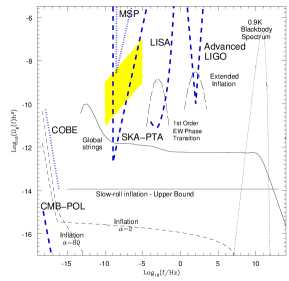
Figure 2: Predicted gravitational wave backgrounds. The top of the figure contains current and predicted limits placed on the gravitational wave background from millisecond pulsar timing, LISA and advanced LIGO. Figure provided by M. Kramer.

Stringent limits have already been placed on the energy density of a stochastic background using the timing residuals of individual pulsars. For a flat GW energy spectrum that is centred on some frequency $f$ and has a bandwidth also equal to $f$ then an upper limit on the energy density ($\rho_{g}$) of a GW background can be obtained from (Detweiler 1979)

$$\rho_{g}<\frac{243}{208}\frac{\pi^{3}f^{4}}{G}\langle R^{2}(t)\rangle$$ (2)

where $G$ is Newton’s gravitational constant and $\langle R^{2}(t)\rangle$ the rms timing residual. Romani & Taylor (1983) obtained an upper limits on the equivalent mass density in GWs in frequency ranges between $0.7\times 10^{-8}$ and $6\times 10^{-8}$ Hz and concluded that, at the present epoch, the mass density of the universe is not dominated by GWs of frequency $\sim 10^{-8}$ Hz.

The expected power spectrum for cosmological models was shown by Blandford et al. (1984) to be

$$P_{g}(f)=\frac{G\rho_{g}(f)}{3\pi^{3}f^{4}}=\frac{H_{0}^{2}}{8\pi^{4}}\Omega_{g}f^{-5}$$ (3)

in which $\rho_{g}(f)$ is the energy density of the stochastic background at frequency $f$, $H_{0}=100h_{0}$ km s^-1 Mpc^-1 is the Hubble constant and $\Omega_{g}$ the fractional energy density in GWs per logarithmic frequency interval. Therefore, if $\Omega_{g}$ is constant then $P(f)\propto f^{-5}$. The index of this power-law ($\alpha=5$) should be contrasted with $\alpha=0$ for white noise and $\alpha=2\rightarrow 4$ expected for clock instabilities, ephemeris errors, interstellar propagation effects and pulsar rotational instabilities (see Stinebring et al. 1990). Stinebring et al. (1990) used seven years of observations to place rigorous upper bounds on the stochastic background. Using a similar method and seven years of data for PSR B1855+09 allowed Kaspi, Taylor & Ryba (1994) to place a limit of $\Omega_{gw}h_{0}^{2}<6\times 10^{-8}$. McHugh et al. (1996) provided a more statistically sound method to obtain that $\Omega_{gw}h_{0}^{2}<10^{-6}$. Their result is independent of the assumption of a flat spectrum for $\Omega_{gw}(f)$.

An astrophysical background would be formed by GW radiation from supermassive black holes. Current theories suggest that galaxies contain a central black hole of mass $\stackrel{{\scriptstyle>}}{{{}_{\sim}}}10^{6}$ M_⊙. As many galaxies are observed to be merging, the existence of a binary black hole system in a merger remnant is likely. If the binary loses enough energy and angular momentum then it may enter a regime where gravitational radiation alone can bring about inspiral and coalescence (Rajagopal & Romani 1995). During an inspiral the GWs will sweep through a range of frequencies. The detection of such events clearly depends upon the rate of occurrence and the amplitude and frequencies of the GWs produced. The possibility of detecting a stochastic background of such events with pulsar timing was described by Rajagopal & Romani (1995).

This work was continued by Jaffe & Backer (2003) who find that the spectrum of a stochastic background of black hole binary systems has a characteristic strain of $h_{c}(f)\sim 10^{-16}(f/yr^{-1})^{-2/3}$ which is just below the detection limit from recent analyses of pulsar timing measurements (see Figure 3). Even though the amplitude of this spectrum was considered too high by Wyithe & Loeb (2003), this background is likely to dominate over cosmological stochastic backgrounds and is therefore the most likely background to be detected using a pulsar timing array. The actual background reached can be determined from the slope of the spectrum which will indicate whether we are observing a coalescing population or other sources of stochastic GWs.

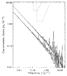
Figure 3: Characteristic strain spectrum for different models of a GW background formed due to merging black-hole binary systems. The dashed line gives the current best limits on the background from pulsar timing observations and the dotted line provides the expected limits from the pulsar timing array after $\sim$ 8 years of operation. Figure obtained from Jaffe & Backer 2003.

4 Individual sources

A periodic source of gravitational radiation will produce a periodic shift in the pulse arrival time. Sufficient GW amplitudes and frequencies that can potentially be detected using a pulsar timing array are predicted to occur from a supermassive black hole binary system in a nearby galaxy (or in the centre of our Galaxy). The expected signature for a supermassive black hole binary system with a circular orbit is given by (Jaffe & Backer 2003)

$$h\approx 4.4\times 10^{-17}m_{8}^{5/3}P_{yr}^{-2/3}d_{Gpc}^{-1}\frac{q}{(1+q)^{2}}$$ (5)

where $h$ is an order-of-magnitude estimate of the strain amplitudes, $m_{8}$ is the total mass of the system in units of $10^{8}$M_⊙, $P_{yr}$ the observed GW period in years, $d$ the distance to the emitter from the Earth in GPc and $q$ is the mass ratio ($q<1$). They also find that the power radiated along the axis of the orbit is eight times that for an edge-on view. The actual effect on the pulsar arrival times will depend upon the angle between the pulsar GW source and the pulsar; a pulsar lying along the line of sight to the GW source will experience no effect.

Lommen & Backer (2001) searched for gravitational radiation from Sagittarius A^∗ which had been postulated to be a massive black-hole binary system (see e.g. Zhao, Bower & Goss 2001). They calculated that the expected effect would be about $\sim$ 10ns in the timing residuals of PSRs B1937$+$21 and J1713$+$0747 which is too small to be detectable with current data. Lommen & Backer (2001) tabulated the expected timing residuals for postulated binary massive black holes in nearby galaxies assuming an equal-mass binary system with an orbital period of 2000 days. If we can identify structures with amplitudes of $\sim$100 ns in the timing residuals then meaningful constraints can be placed on $\sim$10 nearby sources.

The expected signature for the timing residuals for the more general case of a coalescing, binary system in an eccentric orbit was presented in Jenet et al. (2003). The effect depends upon the orbital parameters (including the orbital inclination angle), masses, source distance and the opening angle between the source and the pulsar relative to Earth. Jenet et al. (2004) attempted to detect GWs emitted by the proposed supermassive binary black hole system in 3C66B (Sudou et al. 2003). The expected signature in the timing residuals of PSR B1855+09 are two sinusoids, one with an amplitude $\sim 5\mu s$ and a period of 0.88 years and the other of amplitude $\sim 10\mu s$ with a 6.2 year period (see Figure 4). The two sinusoids occur if the Earth-pulsar line-of-sight is perpendicular to the GW propagation vector as the observed timing residuals will contain information about the source at the current epoch and 4000 years ago (the distance to PSR B1855+09 from Earth is 4000 lt-yr). No such signature was found.

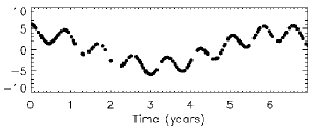
Figure 4: Theoretical timing residuals induced by GWs from 3C66B. No such signature was observed in real pulsar timing residuals (Figure obtained from Jenet et al. 2004)

5 Practical issues

Pulsar timing is affected by the stability of terrestrial clocks, ephemeris errors and the pulsar itself. In order to make a definitive detection of gravity waves then a timing array requires a minimum of five pulsars spread over the sky (see Foster & Backer 1990). One pulsar is required to confirm the stability of terrestrial clocks, three widely spaced pulsars are necessary to solve for an error in the solar system ephemeris and the fifth pulsar to place an upper limit on the GW background. To solve completely for all the available information about the background, more pulsars are required.

The pulse arrival times must be determined to high precision (current timing array projects are aiming to achieve a precision between $10^{-9}$ and $10^{-6}$ seconds). The necessary precision can be estimated from (Rajagopal & Romani 1995)

$$h\sim\frac{\delta t}{P_{w}}(N_{obs}T_{obs})^{-1/2}$$ (6)

in which $h$ is the typical strain amplitude of a detectable GW, $N_{obs}$ the number of arrival times measured each year, $T_{obs}$ the total length of time that the pulsar has been observed, $P_{w}$ the period of the GW and $\delta t$ the typical arrival time precision. Such timing is achievable. For example, van Straten et al. (2001) obtained a residual root-mean-square of only 130 ns over 40 months of observing PSR J0437$-$4715. With better instrumentation this precision should be improved. Measuring pulse arrival times with high precision for most MSPs benefits from observing at frequencies of $\sim 3$ GHz or higher to counteract interstellar propagation effects (Rickett 1977). It is also essential that the pulsar’s dispersion measure is known accurately for every observation. To do this, simultaneous multiple frequency observations are required at widely spaced observing frequencies.

The pulsars chosen as part of a timing array must be intrinsically stable. Some pulsars show “timing noise”, a continuous, noise like fluctuation in the rotation rate (for example, Lyne 1999) or glitches, sudden increases in rotation rate (Lyne, Shemar & Graham-Smith 2000). However, the MSPs have been shown to be extremely stable over many years of observing. In fact, the stability of many MSPs rival that of terrestrial atomic time standards (for example, see Lommen 2002).

The power spectrum of the time derivative of the pulsar timing residuals must be obtained in order to obtain detailed information about the stochastic background. Methods for obtaining this power spectrum from the irregularly sampled pulsar timing residuals have been fiercely debated in the literature. Stinebring et al. (1990) developed a method using orthonormal polynomials as basis functions. This work was generalised for multiple pulsar data sets by Kaspi, Taylor & Ryba (1994), but was criticised by Thorsett & Dewey (1996) who developed a technique based on the Neyman-Pearson test. McHugh et al. (1996) subsequently showed the Neyman-Pearson test of hypothesis also cannot, in the general case, provide upper limits on an unknown parameter and suggested the use of a Bayesian formalism.

When forming the power spectrum of the pulsar timing residuals it is important to recall that the residuals were obtained by fitting a model that includes at least the phase, spin-period, its derivative and position to the pulse arrival times. For many MSPs, fits have also been made for the system’s orbital parameters. The fitting procedure therefore removes long-period variations in the arrival times and hence limits on GWs are not valid for GW periods near to the length of the data span (see Backer & Hellings 1986). The transfer function of the pulsar model as a filter was obtained by Blandford, Narayan & Romani (1984) and should therefore be taken into account when studying relatively short data spans.

6 The Australian pulsar timing array

Figure 5: Location of the millisecond pulsars on the sky that are being observed as part of the Australian pulsar timing array project.

Since Februrary 2004, in a collaborative effort between the ATNF and the Swinburne and Caltech universities, we have been observing $\sim$20 millisecond pulsars using the new 680/3100 MHz dual-frequency receiver and a 1400 MHz receiver at the 64-m Parkes radio telescope (see http://www.atnf.csiro.au/research/pulsar/array). We intend to observe each pulsar at 7–10 day intervals over a period of at least five years. For many of these pulsars we already have timing residual rms values less than 1$\mu s$ with observation times of 30 minutes or 1 hour depending upon the brightness of the pulsar. For PSR J0437$-$4715 we currently have 166 dual-frequency observations spanning 125 days which give us, with only rudimentary processing being applied to the data, a timing residual rms of $\sim$500 ns. This short data span already places a limit of $\Omega_{gw}h_{0}^{2}<5\times 10^{-4}$ on any possible existence of a GW background. If we can reduce the timing residual to 100 ns over 5 years then the limit (from a single pulsar) will be $\Omega_{gw}h_{0}^{2}<5\times 10^{-10}$ and will provide tight constraints on gravitational wave backgrounds from merging black holes and cosmic strings.

We have also been developing a software package, superTempo, for processing the arrival times from multiple pulsars simultaneously. The current status of this, and other related projects, may be found on our web-site.

7 Conclusion

It is likely that gravitational waves will be detected within the next few years by world-wide pulsar timing array projects. As a by-product of these investigations stringent checks will also be placed on terrestrial time standards and the solar system ephemeris. The regular dual-frequency observations of multiple pulsars will also provide valuable information about the interstellar medium. Using a pulsar array as a gravitational wave detector is complimentary to other searches currently being designed that are attempting to detect much shorter-period GWs.

References

- Backer & Hellings , (1986) Backer D. C., Hellings R. W., 1986, ARA&A, 24, 537
- Blandford, Narayan & Romani , (1984) Blandford R. D., Narayan R., Romani R. W., 1984, JA&A, 5, 369
- Caldwell, Battye & Shellard 1996 , (1996) Caldwell, R. R., Battye, R. A., Shellard, E. P. S., 1996, PhRvD, 54, 7146
- Detweiler, (1979) Detweiler S., 1979, ApJ, 234, 1100
- Foster & Backer , (1990) Foster R. S., Backer D. C., 1990, ApJ, 361, 300
- Foster , (1990) Foster R. S., 1990, PhD thesis, University of California, Berkeley
- Hellings & Downs , (1983) Hellings R. W., Downs G. S., 1983, ApJ, 265, L39
- Jaffe & Backer , (2003) Jaffe A. H., Backer D. C., 2003, ApJ, 583, 616
- Jenet et al., 2004 , (2004) Jenet F. A., Lommen A., Larson S. L., Wen L., 2004, ApJ, 606, 799
- Kaspi, Taylor & Ryba , (1994) Kaspi V. M., Taylor J. H., Ryba M., 1994, ApJ, 428, 713
- Lommen & Backer , (2001) Lommen A. N., Backer D. C., 2001, ApJ, 562, 297
- Lommen , (2002) Lommen A. N., 2002, in Neutron Stars, Pulsars, and Supernova Remnants. p. 114
- Lyne, (1999) Lyne A. G., 1999, in Pulsar Timing, General Relativity and the Internal Structure of Neutron Stars, 141
- Lyne, Shemar & Graham-Smith , (2000) Lyne A. G., Shemar S. L., Graham-Smith F., 2000, MNRAS, 315, 534
- Maggiore , (2000) Maggiore M., 2000, Phys. Rep. , 331, 283
- Manchester & Taylor , (1977) Manchester R. N., Taylor J. H., 1977, Pulsars. Freeman, San Francisco
- McHugh et al. , (1996) McHugh M. P., Zalamansky G., Vernotte F., Lantz E., 1996, Phys. Rev. D, 54, 5993
- Rajagopal & Romani, (1995) Rajagopal M., Romani R. W., 1995, ApJ, 446, 543
- Rickett , (1977) Rickett B. J., 1977, ARA&A, 15, 479
- Romani & Taylor , (1983) Romani R. W., Taylor J. H., 1983, ApJ, 265, L35
- Thorsett & Dewey , (1996) Thorsett S. E., Dewey R. J., 1996, 53, 3468
- Stinebring et al. , (1990) Stinebring D. R., Ryba M. F., Taylor J. H., Romani R. W., 1990, Phys. Rev. Lett, 65, 285
- Sudou et al., , (2003) Sudou, H.; Iguchi, S.; Murata, Y.; Taniguchi, Y., 2003, Sci, 300, 1263
- van Straten et al. , (2001) van Straten W., Bailes M., Britton M., Kulkarni S. R., Anderson S. B., Manchester R. N., Sarkissian J., 2001, Nat, 412, 158
- Wyithe & Loeb , (2003) Wyithe J., Loeb A., 2003, ApJ, 590, 691
- Zhao, Bower & Goss , (2001) Zhao, J; Bower G. C., Goss, W. M., 2001, ApJ, 547, L29