PSR J1022+1001: Profile Stability & Precision Timing

Abstract

We present an investigation of the morphology and arrival times of integrated radio pulses from the binary millisecond pulsar PSR J1022+1001. This pulsar is renowned for its poor timing properties, which have been postulated to originate from variability in its average pulse profile. Although a sub-class of long-period pulsars are known to exhibit mode changes that give rise to very large deviations in their integrated profiles, this was the first millisecond pulsar thought to have an unstable mean profile. As part of a precision timing program at the Parkes radio telescope we observed this pulsar between January 2003 and March 2004 using a coherent de-dispersion system (CPSR2). A study of morphological variability during our brightest observations suggests that the pulse profile varies by at most a few percent, similar to the uncertainty in our calibration. Unlike previous authors, we find that this pulsar times extremely well. In five minute integrations of 64 MHz bands we obtain a weighted RMS residual of just 2.27 $\mu$s. The reduced $\chi^{2}$ of our best fit is 1.43, which suggests that this pulsar can be timed to high accuracy with standard cross-correlation techniques. Combining relativistic constraints with the pulsar mass function and consideration of the Chandrasekhar mass limit on the white dwarf companion, we can constrain the inclination angle of the system to lie within the range $37^{o}<i<56^{o}$. For reasonable pulsar masses, this suggests that the white dwarf is at least 0.9 M_⊙. We also find evidence for secular evolution of the projected semi-major axis.

1 Introduction

Pulsar timing is a highly versatile experimental technique that is used to provide estimates of everything from the age and magnetic field strengths of pulsars, allowing population studies (Lyne et al., 1985; Lorimer et al., 1993), to micro-arc-second positions and tests of relativistic gravity (van Straten et al., 2001). Central to the technique is the maxim that pulsars have average pulse profiles that are inherently stable (Helfand et al., 1975), which can be cross-correlated with a template to provide accurate times of arrival (Manchester & Taylor, 1977). Once corrections are made to account for the Earth’s position with respect to the solar system barycentre, a model can be fit to the data, transforming pulsars from astrophysical curiosities into powerful probes of binary evolution and gravitational theories. One spectacular example is the recently-discovered double pulsar system (Lyne et al., 2004).

The discovery of the millisecond pulsars PSR B1937+21 and B1855+09 (Backer et al., 1982; Segelstein et al., 1986) and their subsequent timing (Kaspi et al., 1994) revealed that millisecond pulsars were very rotationally stable, rivaling the best atomic clocks. Their lower magnetic fields appeared to give rise to a fractional stability that far exceeded that of the normal pulsar population (Arzoumanian et al., 1994). This stability, combined with their small rotation periods, gives the millisecond pulsars sub-microsecond timing potential provided sufficient signal-to-noise ratio (S/N) pulse profiles can be recorded. This provides interesting limits on a wide range of astrophysical phenomena (Stairs, 2004).

An array of accurately timed MSPs can even be used to constrain cosmological models and search for long-period (nHz) gravitational waves (Foster & Backer, 1990). Such an array requires frequent observations of a selection of pulsars that are known to time to a precision of less than 1 $\mu$s, preferably in two or more radio frequency bands. Implementation of such an array would provide an opportunity to directly detect gravitational radiation in a regime that complements the sensitivity range of ground-based detectors, to test the accuracy of solar system ephemerides and to construct an entirely extra-terrestrial time scale. The question of whether a suitable sample of millisecond pulsars positioned throughout the entire celestial sphere can be selected from the pulsar catalogue (Hobbs et al., 2004) is under active assessment, through a collaboration between the Australia Telescope National Facility and Swinburne University of Technology.

The feasibility of a timing array depends in part upon the intrinsic rotational stability of the MSPs and their lack of pulse profile variation. Cognard & Backer (2004) have recently discovered a “glitch” in the millisecond pulsar PSR B1821–24, similar to those discovered in younger pulsars (Shemar & Lyne, 1996). Perhaps more disturbingly, Kramer et al. (1999) report that the binary millisecond pulsar PSR J1022+1001 exhibits pulse shape variations that ruin its timing. Studies conducted by Kramer et al. (1999); Ramachandran & Kramer (2003) argue that the pulsar exhibits significant changes in its pulse morphology on $\sim$5 minute time scales and narrow bandwidths. They interpreted these variations as the source of the pulsar’s unusually poor timing properties. By modeling the profile with Gaussian components, Kramer et al. (1999) improved the timing and argued that the trailing component of the pulse was more stable than the leading component.

The precision with which astronomers can predict pulse arrival times has been steadily improving over the past few decades with the advent of new technology and methodology. The charged interstellar medium disperses radio pulses and broadens the pulse profile across finite receiver bandwidths. Astronomers crave both the wide bandwidths that permit high S/N integrated profiles, and the resolution of sharp features that permit strong cross-correlation with a standard template in order to minimise timing errors. Pulsar astronomy has always benefited from adopting new technologies that give increased time resolution and help defeat the deleterious effect of the interstellar medium on the propagation of radio pulses.

Incoherent devices such as analogue filter-banks are prone to systematic errors due to interstellar scintillation and imperfect frequency responses. Digital spectrometers can overcome some of these inadequacies but Hankins & Rickett (1975) described a computational technique (coherent de-dispersion) that removes pulse dispersion “perfectly” almost three decades ago. Unfortunately, at the time, computational hardware was not capable of processing all but the most modest of bandwidths. The exponential growth of computational power has permitted the development of new pulsar instruments that are capable of coherently de-dispersing large bandwidths in near real time. Such an instrument is CPSR2, a baseband recorder that permits near-real time coherent de-dispersion of 2$\times$64 MHz bands using a cluster of high-end workstations (Bailes, 2003). These new instruments represent the best opportunity to study small variations of integrated pulse profiles because they deliver an immunity against systematic errors induced by narrow-band scintillation and dispersion measure smearing. They also provide full polarimetry and multi-bit digitisation, radio frequency interference rejection and the opportunity to apply accurate statistical corrections that help eliminate systematic errors induced by discretisation(Jenet & Anderson, 1998).

Motivated by the arrival of CPSR2, we have commenced a timing campaign of the best millisecond pulsars in an effort to make progress towards the aims of the timing array. PSR J1022+1001 was included because of its high flux density, and the paucity of better candidates at the hour angle it is visible from the Parkes radio telescope. PSR J1022+1001 is a recycled or millisecond pulsar with a pulse period of approximately 16 ms. It orbits once every 7.8 days in a binary system with a companion whose minimum mass can be derived from the pulsar mass function, Eqn 1, if we assume that the orbit is face on and the pulsar has a mass of 1.35 M_⊙.

$$f(m_{\rm p},m_{\rm WD})={{m_{\rm WD}^{3}}\sin^{3}i\over{(m_{\rm p}+m_{\rm WD})^{2}}}={{4\pi^{2}}\over{G}}{{a^{3}\sin^{3}i}\over{P_{\rm b}^{2}}}$$ (1)

Here $m_{\rm p}$ and $m_{\rm WD}$ refer to the mass of the pulsar and white dwarf respectively, $i$ is the inclination angle of the orbit, $P_{\rm b}$ is the orbital period and $G$ is Newton’s gravitational constant. For PSR J1022+1001, this corresponds to a mass of at least 0.7 M_⊙.

Measurements of the dispersion measure along the line of site to the pulsar, combined with the Taylor & Cordes (1993) galactic electron density model, place PSR J1022+1001 at a distance of roughly 600 pc from the sun, making it a relatively nearby source. Accurate timing of this pulsar could therefore lead to a greater knowledge of its orientation, companion masses, distance (via parallax) and proper motion. Unfortunately, this pulsar is very near the ecliptic plane and hence pulsar timing is only good at accurately constraining its position in one dimension. It is therefore a good target for very long baseline interferometry, as this could accurately determine the position and proper motion in ecliptic latitude.

In this paper we present an analysis of the first 15 months of CPSR2 observations of PSR J1022+1001, demonstrating that this pulsar can be timed to high accuracy using standard techniques. In section 2 we describe the observing system and methodology, followed by a description of our data reduction scheme, including polarimetric calibration. Section 3 describes the results of a search within our data set for variations of the type reported by Kramer et al. (1999). Pulse arrival times calculated from this data set are analysed in section 4, followed by a summary of the newly derived pulsar spin and binary system parameters, including those that may become significant in the future. In section 5 we discuss the implications of our work for this pulsar and precision timing programs in general.

2 Observations

2.1 Instrumentation

The second Caltech Parkes Swinburne Recorder (CPSR2) is a baseband recording and online coherent de-dispersion system that accepts 4$\times$64 MHz intermediate frequency bands (IFs). Using the in-built supercomputer, data can be processed either in real time if the pulsar has a dispersion measure (DM) less than approximately 50 pc cm^-3 at a wavelength of 20 cm, or recorded to disk and processed offline. This allows a large amount of flexibility in observing methodology. CPSR2 was commissioned in August 2002 and has been recording data on a regular basis since about November 2002. Observing sessions are primarily conducted using a standard configuration consisting of two independent 64 MHz bands, each with two orthogonal linear polarisations. The down-conversion chain is configured to make both bands contiguous, at centre frequencies of 1341.0 and 1405.0 MHz. In addition, a small number of observations are made at the widely separated frequencies of 3000.0 MHz and 685.0 MHz. After down-conversion and filtering to create band-limited signals, each IF is fed into the CPSR2 Fast Flexible Digitiser board which performs real, 2-bit Nyquist sampling. The digitisation process generates a total of 128 million bytes of data every second. These samples are fed via Direct Memory Access (DMA) cards to two high-speed computers that divide the data into discrete blocks which are distributed via gigabit ethernet to a cluster of client machines for reduction using a software program called PSRDISP (van Straten, 2003). PSRDISP implements software-based coherent de-dispersion (Hankins & Rickett, 1975), assuming prior knowledge of the DM along the line of sight to the pulsar and the validity of the tenuous plasma dispersion law.

2.2 Summary of Observations

Observations were conducted at the Parkes radio telescope over a period of around 400 days between January 2003 and February 2004. The central beam of the Parkes Multibeam receiver (Staveley-Smith et al., 1996) was originally used at the front end, providing a system temperature of approximately 21K at 20 cm. The Multibeam receiver was removed for maintenance in October 2003 and all 20 cm data since this date were recorded using the refurbished, wide-band H-OH receiver whose observable band encompasses that of the Multibeam receiver. The H-OH system is slightly less sensitive than the Multibeam, with a system temperature of 25K at 20 cm wavelengths. In addition, a new coaxial dual-band 10/50 cm receiver system was installed in place of the Multibeam. During the 2004 observing sessions, data were taken with this system in order to expand our frequency coverage for the purposes of dispersion measure monitoring. Preliminary system temperature measurements of the coaxial system yield values of 30 K and 40 K for the 10 cm and 50 cm feeds respectively.

Scheduled observing sessions were typically a few days in duration, occurring once or twice a month. Individual tracks of PSR J1022+1001 vary from approximately 15 minutes to a few hours in duration. The data are somewhat biased towards episodes of favourable scintillation as this allows the most efficient use of limited telescope time. In addition to the on-source tracks, most observations were immediately preceded or followed by a short (2 minute) observation, taken 1 degree south of the pulsar position, during which the receiver noise source was driven with a square wave at a frequency of 11.122976 Hz. These calibration tracks were used to characterise the polarimetric response of the signal chain so that corrections to the observed Stokes parameters could be made during data reduction. Observations of the radio galaxy 3C218 (Hydra A) were also taken at approximately monthly intervals (though often only at 20 cm) and used to calibrate the absolute flux scale of the observing system.

2.3 Data Reduction

Data from each dual-polarisation band were reduced to a coherent filter bank with 128 spectral channels, each 0.5 MHz wide, corresponding to an effective sampling time of 2 $\mu$s. 1024 phase bins were stored across the pulse profile, yielding a time resolution for PSR J1022+1001 of about 15 $\mu$s per bin. Each individual data block recorded by CPSR2 represents 16.7 seconds of data (1 Gigabyte of 2-bit samples). These blocks can later be combined to form integrated profiles. For this purpose the authors use the application set provided with the PSRCHIVE (Hotan et al., 2004) scheme. Due to the IERS practice of retrospectively publishing corrections to the rotation rate of the Earth, the data presented in this paper are that for which corrections to the solar system barycentre could be accurately made at the time of preparation. Observations of PSR J1022+1001 are ongoing.

2.4 Processing & Calibration

The set of 16.7 second PSR J1022+1001 integrations were summed to a total integration time of 5 minutes. These data were calibrated to account for the polarimetric response of the observing system, then all frequency channels and Stokes parameters were combined to form a single total intensity profile corresponding to each 5 minute integration. All of the receiver systems used during observations of PSR J1022+1001 are equipped with orthogonal linear feed probes, so the recorded polarisation products were corrected for relative gain and phase. Off-source calibrator observations were used to compute the relative gain and phase terms for each receiver system at the epoch of the observation, using a simple case of the scheme described by van Straten (2004). We do not attempt to correct for more subtle errors arising from cross-contamination between the two probes, primarily because sufficiently accurate models of all three receiver systems are not yet available. In the case of the central beam of the Multibeam receiver, existing models indicate that imperfections in the orthogonality of the two feed probes may be as large as several degrees (van Straten, 2004). These imperfections break the fundamental assumption of orthogonality made when applying a simple complex gain correction and induce errors in the calculated total intensity of order 1-2 % (Ord et al., 2004). Errors of this magnitude are only present in the profile at phases where the fractional polarisation is close to unity.

3 Pulse Profile Stability

PSR J1022+1001 has an interesting profile morphology. At 20 cm the profile consists of two sharp peaks (the principle components), separated by about 0.05 phase units but joined by a bridge of emission (Fig 1). This characteristic double-peaked shape was critical to the analysis performed by Kramer et al. (1999), who make an effort to characterise variations in the relative amplitude of the two components by normalising against one or the other and computing ratios of their height. The trailing pulse component is observed to possess almost 100 % linear polarisation (Ord et al., 2004; Stairs et al., 1999; Xilouris et al., 1998), whilst the leading component corresponds to a local minimum in the linear polarisation fraction which is near zero (Fig 1). The profile also changes rapidly as a function of frequency, only the leading component is visible at a wavelength of 10 cm (Fig 2) and the amplitude ratio at 50 cm (Fig 3) is nearly half that measured at 20 cm (Fig 1). This spectral index variation within the profile and the highly asymmetric nature of the polarised flux in the principle components, combined with the fact that PSR J1022+1001 is prone to strong episodes of scintillation, means that arrival time analysis over broad frequency bands is easily subject to the introduction of systematic errors. It also complicates any search for variability by exacerbating the effect of instrumental imperfections, especially those associated with polarimetry.

Figure 1: PSR J1022+1001 average profile at a wavelength of 20 cm, formed from data taken with the central beam of the Parkes Multibeam receiver. The profile in the lower panel has been calibrated for relative instrumental gain and phase. It has a centre frequency of 1341.0 MHz and covers a bandwidth of 64 MHz. The solid curve represents total intensity (Stokes I), the dashed curve represents linearly polarised emission and the dotted curve represents circularly polarised emission. Note the high degree of linear polarisation in the trailing component. The relative (not absolute) position angle of the linearly polarised radiation is shown in the top panel. This profile has been calibrated against the flux of Hydra A (3C218).

Figure 2: PSR J1022+1001 average profile at a wavelength of 10 cm, formed from data taken with the new coaxial 10/50 cm receiver system at Parkes. Again, the profile has been calibrated for relative gain and phase. It has a centre frequency of 3000.0 MHz and covers a bandwidth of 64 MHz. Note the small degree of polarisation and the complete absence of the trailing pulse component. Flux calibrator observations were not made at the time these data were recorded, thus the amplitude scale is arbitrary.

Figure 3: PSR J1022+1001 average profile at a wavelength of 50 cm, formed from data taken with the new coaxial 10/50 cm receiver system at Parkes. Again, the profile has been calibrated for relative gain and phase. It has a centre frequency of 685.0 MHz and covers a bandwidth of 64 MHz. Note that the trailing component is almost 100 % linearly polarised and significantly stronger than the leading component. Flux calibrator observations were not made at the time these data were recorded, thus the amplitude scale is arbitrary.

3.1 Profile Normalisation

In order to directly compare multiple integrated profiles from the same pulsar, brightness changes due to interstellar scintillation must be taken into account. This involves scaling or normalising each profile by finding a characteristic value associated with the source flux during the observation and adjusting the measured amplitudes to ensure this value remains fixed across all observations. It should be noted that applying a simple relative scaling to all observed profiles masks any intrinsic variability in the total flux of the pulsar; but that is not the subject of this paper. Using the PSRCHIVE (Hotan et al., 2004) development environment, software was constructed to perform tests similar to those described by Kramer et al. (1999). In the process of analysis and testing, we developed a normalisation scheme based on the concept of difference profiles (Helfand et al., 1975).

Kramer et al. (1999) describe a simple method of normalisation in which the characteristic quantity associated with each integration is taken to be the amplitude of one of the two component peaks. All the amplitudes in the profile are scaled by the constant factor required to give the chosen phase location the value of unity. In the case of PSR J1022+1001, there is a choice as to which peak will be used as the reference. An alternative characteristic quantity is the total flux under the profile, or within a particular phase range. This quantity is simply the sum of all the profile amplitudes within the region of interest. Normalising by flux has the advantage that it uses no morphological information (other than the duty cycle of the pulsed emission in our case) and may therefore be better suited to detecting subtle profile variations.

In this paper we compute fluxes after subtracting a baseline level from each profile. A running mean with a phase width of 0.7 units is used to estimate the baseline flux, which is then subtracted from each bin. In order to further reduce our sensitivity to radio frequency interference and other factors that can distort the uniformity of an observed baseline, we normalise only by the flux in the on-pulse region of the profile. This region is defined by an edge detection algorithm that measures when the total flux crosses a threshold level. This edge detection is performed on the standard template profiles at each wavelength and the phase windows so defined are held fixed for the remainder of the analysis. Unfortunately, normalising profiles by flux tends to artificially amplify noisy observations because a noise-dominated profile has a mean (and therefore a total flux after baseline removal) approaching zero. In the data reduction stage it is therefore advantageous to perform a cut on the basis of S/N. This also helps reduce contamination by corrupted profiles. A S/N cut of 100 was deemed the best compromise between retaining a large fraction of the observed profiles and rejecting noise. This cut was applied to the set of 5 minute CPSR2 integrations before any analysis was commenced.

Kramer et al. (1999)’s technique of normalising to the trailing feature has a number of limitations:

• It cannot place any limits on the variability of the feature that is used to normalise the profiles.

• Polarimetric calibration errors are maximised if the chosen component is highly polarised.

• Finite signal to noise profiles will vary due to noise even if there is no intrinsic variability in the pulsar emission, this is true of all components in the pulse.

We prefer our (more robust) flux-based normalisation scheme which normalises by the total flux in the on-pulse region. Flux normalisation allows us to properly identify which (if any) component is varying as it makes no prior assumptions. It also reduces the effect of poor calibration by averaging over the entire profile. There will still be a background of variability due to noise, but it will be spread uniformly.

3.2 The Difference Profiles

In order to detect subtle changes in pulse shape, it is possible to subtract the amplitudes of a high S/N standard template profile from an appropriately scaled and aligned copy of a given integration. This procedure should yield Gaussian noise if the observed profile precisely matches the standard; any morphological deviations will protrude above the resulting baseline. Before differences can be computed however, the observed profiles must be normalised to a standard template. We choose to normalise all profiles according to the amount of flux in the on-pulse region, as described above. In addition, cross-correlation methods were used to determine relative shifts, after which the observed profiles were rotated to align with the standard template. Because profile variability studies are sensitive to errors in polarimetric calibration, the difference profile analysis was performed on both the calibrated and uncalibrated profiles. Only the 20 cm and 50 cm wavelengths had a sufficient number of high S/N profiles to make a difference profile study possible.

Figs 4 - 7 show difference profiles computed from the CPSR2 observations at a wavelength of 20 cm, while Figs 8 & 9 show the 50 cm results. The number of calibrated profiles is less than or equal to the corresponding number of uncalibrated profiles, as not all observations have corresponding calibration tracks.

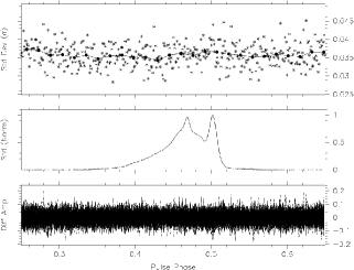
Figure 4: The bottom panel shows superposed morphological difference profiles of 97 five minute total intensity (uncalibrated) integrations at a sky frequency of 1405.0 MHz. The middle panel shows the mean profile. The top panel shows the standard deviation of each phase bin (stars) in the difference profiles displayed in the bottom panel and a series (filled circles) representing the mean value of the standard deviation in 64 windows, connected by lines, to aid perception of trends in the data.

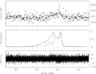
Figure 5: As in Fig 4, superposed morphological difference profiles of 50 total intensity (calibrated) integrations at a sky frequency of 1405.0 MHz. The dashed line under the solid curve in the middle panel represents the total polarised emission in the mean profile.

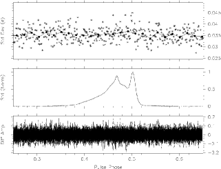
Figure 6: As in Fig 4, superposed morphological difference profiles of 102 total intensity (uncalibrated) integrations at a sky frequency of 1341.0 MHz

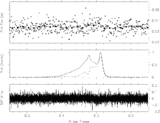
Figure 7: As in Fig 5, superposed morphological difference profiles of 37 total intensity (calibrated) integrations at a sky frequency of 1341.0 MHz

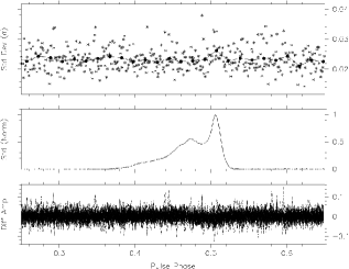
Figure 8: As in Fig 4, superposed morphological difference profiles of 31 total intensity (uncalibrated) integrations at a sky frequency of 685.0 MHz

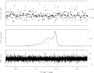
Figure 9: As in Fig 5, superposed morphological difference profiles of 31 total intensity (calibrated) integrations at a sky frequency of 685.0 MHz

As all figures show, the difference profiles are almost consistent with noise, with no alarming peaks near the leading or trailing components. This can be seen from both the difference profiles and their standard deviations. The only evidence for variability comes from Fig 5 where $\sim$2 % variability above the noise floor can be seen near the trailing component. However, these variations are not present in Fig 4, which represents the same data set in the absence of polarimetric calibration. It would seem that the calibration procedure itself is capable of inducing profile instability, which is perhaps not surprising considering the simplicity of the model used to correct for receiver imperfections. In addition, CPSR2 has dynamic level setting that ensures the mean counts are equal in both polarisations. Provided the effective system temperature in the two polarisations is similar, calibration is almost unnecessary to form an accurate total intensity profile. It therefore seems a bizarre coincidence that these variations could be removed by simply neglecting to calibrate the data, and that they correspond to the maximum polarisation fraction in the profile. The simplest interpretation is that across 64 MHz bandwidths, this pulsar’s mean profile is stable and that we are simply seeing the limitations of our calibration procedure.

3.3 Peak Ratio Evolution

Kramer et al. (1999) infer the presence of smooth variations in the relative amplitudes of the principle components on time scales of a few minutes to an hour or more by calculating peak amplitude ratios and demonstrating that they evolve at a level significantly above the uncertainty in the measurement. They also note that instances of such smooth variation may not be common and that the time scales involved can change from one data set to another.

As a secondary check, we computed similar amplitude ratios to that of Kramer et al. (1999) for our high S/N profiles. A S/N cut of 30 was deemed sufficient for this analysis because it is less susceptible to baseline corruption than the difference profile test. The RMS of the off-pulse region in each profile was used as an indication of the error in peak amplitude. The ratio of leading to trailing component amplitude was computed for all profiles and plotted against observation time (see Fig 10 for an example). In addition, mean ratios and their associated standard deviation were computed over the 15 month time span of our data set. These values are presented in Tables 1 and 2.

Frequency (MHz)	Ratio	Std Dev
1405.0	0.97	0.07
1341.0	0.91	0.07
685.0	0.58	0.02

Table 1: Ratio of leading to trailing component for the calibrated data set.

Frequency (MHz)	Ratio	Std Dev
1405.0	0.97	0.06
1341.0	0.90	0.06
685.0	0.58	0.02

Table 2: Ratio of leading to trailing component for the uncalibrated data set.

The evolution of the profile’s components with frequency is quantified in Tables 1 and 2. It is interesting to note that calibration of the data increases the scatter in the measured ratios at higher frequencies, this further supports the notion that the variability observed in Fig 5 and by Kramer et al. (1999) is likely due to errors in the simple model used for polarimetric calibration. This does not seem to be the case at lower radio frequencies, as the calibration procedure has no detectable influence on the computed component ratios at 685.0 MHz. The 50 cm system may simply be better suited to the receiver model used for calibration, however the intrinsic scatter at this frequency is also much smaller so the effect of calibration may be imperceptible. To investigate the evolution of these component ratios in time, the data set was examined by eye in the hope of finding clear indications of non-random evolution between 5 minute integrations. Fig 10 shows the observation that exhibited the most variation. Calibration has little effect on these points. The variation about the mean is small and perhaps insignificant.

Figure 10: Ratios of leading to trailing peak amplitudes during a single 2.5 hour observation taken on September 22, 2003, at a frequency of 1341.0 MHz. The error bars are computed based on the assumption that the amplitude of each peak could vary by the RMS of the noise in the baseline of the profile.

3.4 Summary

The CPSR2 data set suggests that across a bandwidth of 64 MHz, PSR J1022+1001 does not vary significantly. Any instabilities, if present, must also be transitory in nature and therefore extremely difficult to characterise. It is possible that variability with a random or quasi-periodic structure, or small ($<$ 64 MHz) characteristic bandwidth might still be present, but if so it would appear to have little effect on the profile when all frequency channels are combined. Profile instabilities should also be reflected in the timing of the pulsar, which we investigate in the next section.

4 Arrival Time Analysis

Kramer et al. (1999) report that arrival times recorded at the Arecibo, Jodrell Bank and Effelsberg radio telescopes yield a best fit RMS residual of 15-20 $\mu$s when applied to a model of PSR J1022+1001 and the binary system in which it resides. To achieve this RMS residual, a complicated standard template profile consisting of five Gaussian components with floating amplitudes was used, to compensate for supposed intrinsic profile variability. In contrast, the CPSR2 data set yields arrival times (from each 5 minute integration, across multiple radio frequencies) that fit our timing model with a RMS residual of 2.27 $\mu$s. These times of arrival (TOAs) were obtained using a Fourier domain cross correlation process. Simple, static standard template profiles were constructed from the sum total of multiple integrations and the baseline noise was flattened to zero, to decrease spurious self-correlation of the timing profiles with the noise in the standard, which can lead to an RMS that is artificially low. Separate standards were used for each frequency band and were aligned to a common fiducial point. Our 5 minute (uncalibrated) integrations were fit to a model of PSR J1022+1001 using the standard pulsar timing package TEMPO. Fig 11 shows the corresponding timing residuals. It is interesting to note that although the front-end receiver system was changed mid-way through the data set, there does not seem to be any large systematic offset between the two receivers and no jumps were used to fit across the boundary. Changes in cable length or amplifier response between the two systems must have some impact on the assignment of arrival times, however it would appear that the offset is too small to measure in this data set.

Figure 11: Timing residuals from all 5 minute integrations with S/N in excess of 30 and timing error less than 7 $\mu$s. The RMS residual is 2.27 $\mu$s and the reduced $\chi^{2}$ of the weighted fit is 1.43. The vertical scale is an order of magnitude better than arrival times presented by Kramer et al. (1999) who saw residuals as large as 400 $\mu$s.

A binary model of the type described by Blandford & Teukolsky (1976) was used to model the spin-down characteristics of PSR J1022+1001 and the perturbations introduced by its companion. A list of fitted parameters and their corresponding values (with error estimates) is presented below (Table 3). The errors in each TOA were uniformly scaled by a factor of 1.195 before fitting, to ensure the reduced $\chi^{2}$ per degree of freedom was equal to unity. This is necessary to produce better error estimates for the fitted parameters. Sky position is shown in both Ecliptic and Equatorial (J2000) coordinates. PSR J1022+1001 lies in the ecliptic plane, making it difficult to determine the ecliptic latitude ($\beta$) accurately through timing measurements. This accounts for the relatively high error in our measurement of $\beta$ in Table 3. In addition, the CPSR2 data has a time baseline of only 15 months, whereas the data presented by Kramer et al. (1999) extends over more than 4 years. As a consequence, we do not fit for a proper motion in our model, choosing instead to hold this parameter fixed at the value of –17 $\pm$ 2 mas yr^-1 quoted by Kramer et al. (1999). With proper motion thus constrained, we obtain a significant estimate for the parallax of the system. Given the short temporal baseline of our data set, this parallax estimate should be considered preliminary and it is included because it appears significant.

Parameter	Value
Ecliptic Lon. ($\lambda$) (deg)	153.86589029 (4)
Ecliptic Lat. ($\beta$) (deg)	-0.06391 (6)
Proper Motion in $\lambda$ (mas yr-1)	-17 (2) ∗
Parallax (mas)	3.3 (8)
Period (ms)	16.4529296931296 (5)
Period Derivative ($10^{-20}$)	4.33 (1)
Period Epoch (MJD)	52900
Dispersion Measure (cm-3pc)	10.25180 (7)
Projected Semi-Major Axis (lt-s)	16.7654148 (2)
Eccentricity	0.00009725 (3)
Time of Periastron Passage (MJD)	52900.4619 (3)
Orbital Period (days)	7.805130160 (2)
Angle of Periastron (deg)	97.73 (1)
Right Ascension ($\alpha$)	10:22:58.015 (5)
Declination ($\delta$)	+10:01:53.2 (2)
Number of TOAS	555
Total $\chi^{2}$	545.74
RMS Timing Residual ($\mu$s)	2.27
MJD of first TOA	52649
MJD of last TOA	53109
Total Time Span (days)	460

Table 3: PSR J1022+1001 Blandford & Teukolsky (1976) timing model parameters derived from 15 months of CPSR2 observations. The error in the last significant digit is given in parentheses after the value. (^∗ This value was given by Kramer et al. (1999))

Fig 11 shows that PSR J1022+1001 has benefited from more regular observations in recent months. There are only a few small groups of points in the earliest part of the data set. This is another reason for not including proper motion in the model, as the small number of points observed during the beginning of 2003 would unreasonably dominate the fit. Parallax measurements are sensitive to day of year coverage more than total observing time, so it is still possible that the value of 3.3 $\pm$ 0.8 mas is meaningful. It is interesting to note that our parallax measurement implies a distance of only 300 ${}^{+100}_{-60}$ pc, as opposed to the value of 600 pc derived from the Taylor & Cordes (1993) electron density model. Many pulsars within 1 kpc of the Sun are inconsistent with the Taylor & Cordes (1993) model at this level. If the system is indeed only 300 pc from the sun, other secular changes may soon be detectable in the orbital parameters, such as $a\sin i$.

The accuracy with which we have been able to time this pulsar affords the chance to derive new limits on several physical parameters. Of particular interest is the possible presence of orbitally modulated Shapiro delay as the distance each pulse must travel into the companion star’s gravity well changes throughout the 7.8 day orbit. Whilst fitting for the Shapiro delay parameters $m_{\rm WD}$ and $i$ is not directly possible due to the small amplitude of their timing signature, a statistical analysis of the effect these parameters have on the $\chi^{2}$ of the fit can still reveal important information. The parameters derived from our Blandford & Teukolsky (1976) model were incorporated into a model (Damour & Deruelle, 1985, 1986) that includes the two Shapiro delay parameters. This new model was used to create a $\chi^{2}$ map for varying companion masses and inclination angles (Fig 12). This map allows us to place upper and lower bounds on the likely inclination angle, although it does not tightly constrain the companion mass. Based on 2-$\sigma$ Shapiro delay contours, $\cos i>$ 0.56. Assuming a neutron star mass of 1.35 M_⊙ and a white dwarf companion (a valid assumption given the small eccentricity of the system), the Chandrasekhar mass limit for the companion constrains $\cos i<$ 0.8. These two limits combined imply that the inclination angle lies between 37^o and 56^o and suggest that $m_{\rm WD}>$ 0.9 M_⊙. This suggests that the initial binary was near the limit required to produce two neutron stars, and that the white dwarf is composed of heavier elements (maybe even ONeMg) than many of the millisecond pulsar companions which are most often He white dwarfs.

Figure 12: Shapiro delay $\chi^{2}$ map. The thick lines represent 1-$\sigma$ contours, followed by 2,3 and 4-$\sigma$ contours on the left hand side. The dashed line represents the mass function constraint, assuming a 1.35 M_⊙ neutron star.

The model parameters presented in Kramer et al. (1999) include a value for the projected semi-major axis of the orbit, $x=a\sin i=$ 16.765409(2) s. Given that the reference epoch of our data set is some 7 years ahead of the corresponding Kramer et al. (1999) epoch, it is possible to compare our value of $x$ in the hope of detecting a significant change as the proper motion of the system alters our line of sight to the plane of the orbit. We find $\dot{x}$ = 0.8 $\pm$ 0.3 $\mu$s yr^-1. Sandhu et al. (1997) show that:

$$\dot{x}=x\cot i(-\mu_{\alpha}\sin\Omega+\mu_{\delta}\cos\Omega){\rm ss}^{-1}$$ (2)

where $\mu_{\alpha}$ and $\mu_{\delta}$ represent the components of proper motion in RA and Dec and $\Omega$ is the longitude of the ascending node. Only the component of $\mu$ in ecliptic longitude was measured by Kramer et al. (1999), but given our constraints on the inclination angle $i$, the only two unknowns in the equation are now $\mu_{\delta}$ and $\Omega$ . If VLBI measurements could provide a value for $\mu_{\delta}$ (and perhaps confirm our detection of parallax), we would be able to place limits on the angle $\Omega$, further constraining the 3-dimensional orientation of the orbit on the sky.

The reduced $\chi^{2}$ of 1.43 indicates that the arrival times are relatively free from unmodeled systematic effects. Increasing the error estimates by 20 % gives a $\chi^{2}$ of unity, which is low by precision pulsar timing standards. Another way to view this low level of systematics is to plot the residual against the arrival time measurement uncertainty for each TOA (Fig 13). With perhaps one exception, there are almost no points many standard deviations from zero.

Figure 13: Model residual plotted as a function of error in arrival time.

Kramer et al. (1999) argue that the leading component of PSR J1022+1001 varies across a characteristic bandwidth of approximately 8 MHz. In order to test this, a separate timing analysis was performed on the 20 cm wavelength data before complete summation of the frequency channels, reducing the bandwidth in each integrated profile to 8 MHz. If the pulsar is varying on these bandwidths and 5 minute time scales, this should lead to an enormous increase in the RMS residual that grossly exceeds the expected factor of $\sqrt{8}$. We find that the RMS residual of these 8 MHz bandwidth arrival times is 6.65 $\mu$s, which is very close to $\sqrt{8}\times 2.27=6.42$ $\mu$s, implying that the increased scatter is consistent with the loss of S/N associated with the reduction in bandwidth. This analysis is strong evidence that there are no profile variations with a characteristic bandwidth of approximately 8 MHz and time scales of a few minutes.

5 Conclusions

PSR J1022+1001 has an interesting pulse profile morphology in terms of characteristic shape, polarimetric structure and evolution with radio frequency. These factors conspire to make it a difficult source to calibrate and analyse. Extensive studies of the morphological differences between 5-minute integrations observed with CPSR2 at the Parkes 64 m radio telescope are consistent with a stable pulse profile. This bodes well for the future of precision timing of both this source and millisecond pulsars in general. Although the RMS residual presented is probably not small enough to make an immediate contribution to any pulsar timing array, lengthier integrations and continued monitoring may yet push the timing of this pulsar below the 1 $\mu$s mark.

We have used our improved timing to place some interesting limits on the geometry of this source which demonstrate that the inclination angle lies within the range $37^{o}<i<56^{o}$. If our parallax is confirmed, this system will make a good target for VLBI observations which could both improve the distance to the pulsar and determine the as yet unknown component of proper motion in the direction of ecliptic latitude. This would provide additional limits on the three dimensional orientation of the orbit via consideration of the change in projected semi-major axis. In the future, limits on $\dot{x}$ will improve and on a 10-year baseline, other relativistic observables may become measurable. We anticipate that with another 20 months of timing, we should be able to obtain a more meaningful parallax and independent proper motion for this source in right ascension. Our error in $\omega$ is only 0.01^o, which suggests that the expected rate of advance of periastron for this source $\dot{\omega}\sim 0.01^{o}{\rm yr}^{-1}$ may be measurable on a 10-year baseline.

Acknowledgments.

Parkes radio telescope is operated by the Australia Telescope National Facility on behalf of the CSIRO. We thank Haydon Knight for observing assistance. AWH is the recipient of an APA and CSIRO postgraduate top-up allowance and thanks Claire Trenham for support and encouragement.

References

- Arzoumanian et al. (1994) Arzoumanian Z., Nice D. J., Taylor J. H., Thorsett S. E., 1994, ApJ, 422, 671
- Backer et al. (1982) Backer D. C., Kulkarni S. R., Heiles C., Davis M. M., Goss W. M., 1982, Nature, 300, 615
- Bailes (2003) Bailes M., 2003, in ASP Conf. Ser. 302: Radio Pulsars Vol. 302, Precision timing at the parkes 64-m radio telescope. p. 57
- Blandford & Teukolsky (1976) Blandford R., Teukolsky S. A., 1976, ApJ, 205, 580
- Cognard & Backer (2004) Cognard I., Backer D. C., 2004, in Combes F., Barret D., Contini T., Meynadier F., Pagani L., eds, SF2A-2004: Semaine de l’Astrophysique Francaise A micro-glitch observed on a recycled millisecond pulsar. EdP-Sciences, France, p. 305
- Damour & Deruelle (1985) Damour T., Deruelle N., 1985, Ann. Inst. H. Poincaré (Physique Théorique), 43, 107
- Damour & Deruelle (1986) Damour T., Deruelle N., 1986, Ann. Inst. H. Poincaré (Physique Théorique), 44, 263
- Foster & Backer (1990) Foster R. S., Backer D. C., 1990, ApJ, 361, 300
- Hankins & Rickett (1975) Hankins T. H., Rickett B. J., 1975, in Methods in Computational Physics Volume 14 — Radio Astronomy Pulsar signal processing. Academic Press, New York, pp 55–129
- Helfand et al. (1975) Helfand D. J., Manchester R. N., Taylor J. H., 1975, ApJ, 198, 661
- Hobbs et al. (2004) Hobbs G., Manchester R., Teoh A., Hobbs M., 2004, in IAU Symposium no. 218, held as part of the IAU General Assembly, 14-17 July, 2003 in Sydney, Australia. The atnf pulsar catalog. Astronomical Society of the Pacific, p. 139
- Hotan et al. (2004) Hotan A. W., van Straten W., Manchester R. N., 2004, Proc. Astr. Soc. Aust., 21, 302
- Jenet & Anderson (1998) Jenet F. A., Anderson S. B., 1998, PASP, 110, 1467
- Kaspi et al. (1994) Kaspi V. M., Taylor J. H., Ryba M., 1994, ApJ, 428, 713
- Kramer et al. (1999) Kramer M., Xilouris K. M., Camilo F., Nice D., Lange C., Backer D. C., Doroshenko O., 1999, ApJ, 520, 324
- Lorimer et al. (1993) Lorimer D. R., Bailes M., Dewey R. J., Harrison P. A., 1993, MNRAS, 263, 403
- Lyne et al. (2004) Lyne A. G., Burgay M., Kramer M., Possenti A., Manchester R. N., Camilo F., McLaughlin M., Lorimer D. R., Joshi B. C., Reynolds J. E., Freire P. C. C., 2004, Science, 303, 1153
- Lyne et al. (1985) Lyne A. G., Manchester R. N., Taylor J. H., 1985, MNRAS, 213, 613
- Manchester & Taylor (1977) Manchester R. N., Taylor J. H., 1977, Pulsars. Freeman, San Francisco
- Ord et al. (2004) Ord S. M., van Straten W., Hotan A. W., Bailes M., 2004, MNRAS, 352, 804
- Ramachandran & Kramer (2003) Ramachandran R., Kramer M., 2003, A&A, 407, 1085
- Sandhu et al. (1997) Sandhu J. S., Bailes M., Manchester R. N., Navarro J., Kulkarni S. R., Anderson S. B., 1997, ApJ, 478, L95
- Segelstein et al. (1986) Segelstein D. J., Rawley L. A., Stinebring D. R., Fruchter A. S., Taylor J. H., 1986, Nature, 322, 714
- Shemar & Lyne (1996) Shemar S. L., Lyne A. G., 1996, MNRAS, 282, 677
- Stairs (2004) Stairs I. H., 2004, Science, 304, 547
- Stairs et al. (1999) Stairs I. H., Thorsett S. E., Camilo F., 1999, ApJS, 123, 627
- Staveley-Smith et al. (1996) Staveley-Smith L., Wilson W. E., Bird T. S., Disney M. J., Ekers R. D., Freeman K. C., Haynes R. F., Sinclair M. W., Vaile R. A., Webster R. L., Wright A. E., 1996, Proc. Astr. Soc. Aust., 13, 243
- Taylor & Cordes (1993) Taylor J. H., Cordes J. M., 1993, ApJ, 411, 674
- van Straten (2003) van Straten W., 2003, PhD thesis, Swinburne University of Technology
- van Straten (2004) van Straten W., 2004, apjss, 152, 129
- van Straten et al. (2001) van Straten W., Bailes M., Britton M., Kulkarni S. R., Anderson S. B., Manchester R. N., Sarkissian J., 2001, Nature, 412, 158
- Xilouris et al. (1998) Xilouris K. M., Kramer M., Jessner A., von Hoensbroech A., Lorimer D., Wielebinski R., Wolszczan A., Camilo F., 1998, ApJ, 501, 286