Calibrating the Nonlinear Matter Power Spectrum: Requirements for Future Weak Lensing Surveys

Abstract

Uncertainties in predicting the nonlinear clustering of matter are among the most serious theoretical systematics facing the upcoming wide-field weak gravitational lensing surveys. We estimate the accuracy with which the matter power spectrum will need to be calibrated in order not to contribute appreciably to the error budget for future weak lensing surveys. We consider the random statistical errors and the systematic biases in $P(k)$, as well as some estimates based on current N-body simulations. While the power spectrum on relevant scales ($0.1\lesssim k/h\,{\rm Mpc}^{-1}\lesssim 10$) is currently calibrated with N-body simulations to about 5-10%, in the future it will have to be calibrated to about 1-2% accuracy, depending on the specifications of the survey. Encouragingly, we find that even the worst-case error that mimics the effect of cosmological parameters needs to be calibrated to no better than about 0.5-1%. These goals require a suite of high resolution N-body simulations on a relatively fine grid in cosmological parameter space, and should be achievable in the near future.

, ,

1 Introduction

Weak gravitational lensing (WL) of distant galaxies is determined by the total matter overdensity along the line of sight. In more technical terms, weak lensing measures the matter power spectrum weighted with a function that depends on the geometry of the lens-deflector-observer system. Therefore, in order to predict the WL signal for a given set of cosmological parameters, one needs to be able to accurately calibrate the matter power spectrum $P(k)$.

The sensitivity of weak lensing surveys peaks at scales of about 10 arcminutes on the sky, corresponding to intervening structures of size $\sim 1h^{-1}\,{\rm Mpc}$ at redshift $\sim 0.5$, which is approximately where the lensing efficiency of distant galaxies peaks (e.g. Jain & Seljak 1997). Therefore, the scales probed are nonlinear and need to be calibrated by N-body simulations. Unfortunately, one cannot afford to restrict the measurements to linear scales for which there are accurate analytical predictions (and which corresponds to scales $\gtrsim 1$ deg. at $z\sim 0.5$), since the information from large scales only is poorly constraining due to cosmic variance (e.g. Huterer 2002).

Therefore, accurate calibration of the fully nonlinear matter power spectrum $P(k)$ is necessary to ensure that the cosmological parameter determination from weak lensing surveys is not compromised. Current accuracy in the matter power spectrum at mildly nonlinear scales is about 5-10% (White & Vale 2004; Heitmann et al. 2004) which is sufficiently small for current surveys (for reviews of weak lensing, see e.g., Bartelmann & Schneider 2001, Van Waerbeke & Mellier 2003, Refregier 2003). However, the accuracy will need to be better for future wide-field surveys. The accuracy and agreement of various N-body simulations is rapidly improving and the currently popular fitting formulae for the power spectrum (e.g. Ma et al. 1999, Jenkins et al. 2001, Smith et al. 2003) will soon be insufficiently accurate and flexible and one will need to resort to a full suite of N-body simulations, interpolating on a grid of cosmological models (and thereafter, perhaps, building a new set of more flexible and accurate fitting formulae).

In this work we consider the requirements of future deep, wide-field WL surveys such as Dark Energy Survey, PanSTARRS, Supernova/Acceleration Probe (SNAP; Aldering et al. 2004) and Large Synoptic Survey Telescope (LSST). For the fiducial model we assume sky coverage of 1000 sq. deg. with 100 galaxies per arcmin². We vary these numbers later to determine the robustness of our results to survey specifications. We assume a flat universe with matter energy density relative to critical $\Omega_{M}=0.3$, dark energy equation of state $w=-1$, and power spectrum normalization $\sigma_{8}=0.9$. We use the spectral index and physical matter and baryon energy densities with mean values $n=1.0$, $\Omega_{M}h^{2}=0.140$ and $\Omega_{B}h^{2}=0.023$ respectively. The parameters whose future accuracy can most benefit from future WL surveys are $\Omega_{M}$, $w$ and $\sigma_{8}$, and we pay particular attention to these three. We do not add any priors whatsoever, since we are considering the efficacy of WL surveys in their own right; moreover, we have checked that reasonable priors (for example, those based on expected accuracies from the Planck experiment) have minimal effect on the three aforementioned parameters and all of our results. Note that we do not consider the time variation in $w$ since the best-measured mode of an arbitrary $w(z)$ is about as well measured as $w={\rm constant}$ (Huterer & Starkman 2003), and it is this particular mode, being the most sensitive to theory systematics, that will drive the accuracy requirements. Hence, it is sufficient to consider the constant $w$ case. Throughout we consider lensing tomography with 10 redshift bins equally spaced between $z=0$ and $z=3$ and use the lensing power spectra on scales $50\leq\ell\leq 3000$. Over this range of multipoles, statistical properties of the lensing fields are nearly Gaussian and, furthermore, complex baryonic effects that are expected to be significant on smaller scales are strongly suppressed (e.g. White 2004, Zhan & Knox 2004). [Cosmological parameter extraction from WL tomography has been extensively discussed in the past, e.g. Hu 1999, Huterer 2002, Hu 2003, Refregier et al. 2003, Takada & Jain 2004, Takada & White 2004, Song & Knox 2004, Ishak et al. 2004.]

The convergence power spectrum at a fixed multipole $\ell$ and for the $i$th and $j$th tomographic bin is given by

$$P_{ij}^{\kappa}(\ell)=\int_{0}^{\infty}dz\,{W_{i}(z)\,W_{j}(z)\over r(z)^{2}\,H(z)}\,P\!\left({\ell\over r(z)},z\right),$$ (1)

where $r(z)$ is the comoving angular diameter distance and $H(z)$ is the Hubble parameter. The weights $W_{i}$ are given by $W_{i}(\chi)={3\over 2}\,\Omega_{M}\,H_{0}^{2}\,g_{i}(\chi)\,(1+z)$ where $g_{i}(\chi)=r(\chi)\int_{\chi}^{\infty}d\chi_{s}n_{i}(\chi_{s})r(\chi_{s}-\chi)/r(\chi_{s})$, $\chi$ is the comoving radial distance and $n_{i}$ is the comoving density of galaxies if $\chi_{s}$ falls in the distance range bounded by the $i$th redshift bin and zero otherwise. We employ the redshift distribution of galaxies of the form $n(z)\propto z^{2}\exp(-z/z_{0})$ that peaks at $2z_{0}=1.0$ (for LSST, we use $2z_{0}=0.7$). The observed convergence power spectrum is

$$C^{\kappa}_{ij}(\ell)=P_{ij}^{\kappa}(\ell)+\delta_{ij}{\langle\gamma_{\rm int}^{2}\rangle\over\bar{n}_{i}},$$ (2)

where $\langle\gamma_{\rm int}^{2}\rangle^{1/2}$ is the rms intrinsic shear in each component which we assume to be equal to $0.22$, and $\bar{n}_{i}$ is the average number of galaxies in the $i$th redshift bin per steradian. The cosmological constraints can then be computed from the Fisher matrix

$$F_{ij}=\sum_{\ell}\,{\partial{\bf C}\over\partial p_{i}}\,{\bf Cov}^{-1}\,{\partial{\bf C}\over\partial p_{j}},$$ (3)

where ${\bf Cov}^{-1}$ is the inverse of the covariance matrix between the observed power spectra whose elements are given by

$${\rm Cov}\left[C^{\kappa}_{ij}(\ell),C^{\kappa}_{kl}(\ell^{\prime})\right]={\delta_{\ell\ell^{\prime}}\over(2\ell+1)\,f_{\rm sky}\,\Delta\ell}\,\left[C^{\kappa}_{ik}(\ell)C^{\kappa}_{jl}(\ell)+C^{\kappa}_{il}(\ell)C^{\kappa}_{jk}(\ell)\right].$$ (4)

assuming that the convergence field is Gaussian, which is a good approximation at $\ell<3000$. We alternatively consider a SNAP-type survey (1000 sq. deg., 100 gal/arcmin²) and an LSST-type survey (15000 sq. deg., 30 gal/arcmin²). The fiducial marginalized accuracies in $\Omega_{M}$, $w$ and $\sigma_{8}$ for the two surveys, without any theoretical systematics, are given in Table 1.

Parameter	SNAP Error	LSST Error
$\Omega_{\rm DE}$	0.008	0.003
$w$	0.052	0.025
$\sigma_{8}$	0.006	0.003

Table 1: Fiducial 1-$\sigma$ errors in $\Omega_{M}$, $w$ and $\sigma_{8}$ for the SNAP-type and LSST-type surveys assuming no systematics. These errors were obtained by marginalizing over all (five) other cosmological parameters.

In Section 2 we assume random errors in the matter power spectrum $P(k)$ and determine their maximal allowed size so that they do not appreciably add to the overall error budget in future surveys. In Section 3 we explore biases due to several specific sources of error, and also consider the worst-case scenario when errors in $P(k)$ conspire to maximally bias the cosmological parameters. We conclude in Section 4.

2 Statistical errors in $P(k)$

First, let us parameterize the deviations in the matter power spectrum around its fiducial value by 30 parameters $\delta\ln P_{i}$ in bins spaced equally in $\log k$ from $k=0.1h\,{\rm Mpc}^{-1}$ to $k=10h\,{\rm Mpc}^{-1}$. More precisely, if $k$ is in the $i$th bin, we allow the variations

$$P(k,z)\rightarrow P(k,z)\left(1+\delta\ln P_{i}\right)$$ (5)

where $\delta\ln P_{i}$ are assumed to be independent gaussian random variables, not determined by the cosmological parameters, with mean zero. Note too that we assume that relative variations in $P(k,z)$, parametrized by $\delta\ln P_{i}$, are independent of $z$. This simplifying assumption is motivated by the fact that the source of error in $\ln P(k,z)$ is imperfect accuracy of N-body simulations, where biases in $\ln P(k,z)$ are likely to be weakly dependent on $z$ in the range relevant for WL. We compute the linear power spectrum using the fitting formulae of Eisenstein & Hu (1999) which were fit to the numerical data produced by CMBFAST (Seljak & Zaldarriaga 1996). We generalize the formulae to $w\neq-1$ by appropriately modifying the growth function of density perturbations. To complete the calculation of the full nonlinear power spectrum we use the fitting formulae of Smith et al. (2003).

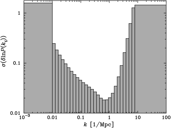
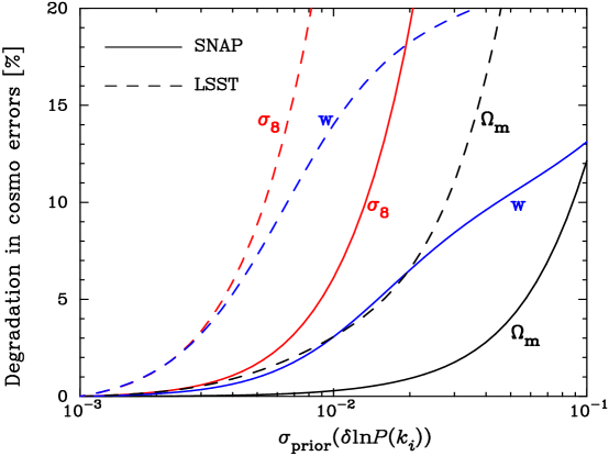
Figure 1: Effects of random statistical error on the power spectrum $P(k)$. In the top panel we represent $P(k)$ in 30 bins distributed uniformly in $\log k$ from $k=0.1$ to $10h\,{\rm Mpc}^{-1}$ and show the unmarginalized accuracy in each band power, $\delta\ln P_{i}$, assuming that the cosmological parameters are perfectly known. It is clear that the scale that is most sensitive to weak lensing measurements is $k\sim 1h\,{\rm Mpc}^{-1}$, and therefore $P(k)$ around this scale needs to be calibrated most accurately. We also find that about 10 band powers of $P(k)$ in the plotted range are independent. The bottom panel shows the increase in the error in cosmological parameters $\Omega_{m}$, $w$ and $\sigma_{8}$ as a function of prior imposed on each of the 10 nuisance parameters $\delta\ln P_{i}$. The solid and dashed curves are the results for SNAP- and LSST-type surveys, respectively. The required accuracy is about $2\%$ from $\sigma_{8}$ and 5-10% from $\Omega_{M}$ and $w$ for SNAP, and about a factor of two more stringent for LSST.

We assume for a moment that all cosmological parameters are precisely known and fixed. The top panel of Figure 1 shows that the unmarginalized accuracies in $\delta\ln P_{i}$ range from a few hundredths to a few tens, except on very small scales. Not surprisingly, the best accuracy is achieved on scales of $\sim 1h\,{\rm Mpc}^{-1}$ to which the lensing power spectra of our interest are most sensitive. From the covariances between different $\delta\ln P_{i}$ (i.e. the off-diagonal components of the Fisher information matrix), we find that only about 10 bins in $P(k)$ are independent – in other words, the weak lensing kernel is broad enough to differentiate only around 10 parameters in $P(k)$ in this range of $k$. We then investigate how accurately these 10 numbers need to be known for the cosmological parameter accuracies not to be affected appreciably. We add equal priors to 10 values $\delta\ln P_{i}$ ($i=1\ldots 10$) in bins spaced equally in $\log k$ from $k=0.1h\,{\rm Mpc}^{-1}$ to $k=10h\,{\rm Mpc}^{-1}$ and marginalize over them, then compute the degradation in the marginalized accuracies of $\Omega_{M}$, $\sigma_{8}$ and $w$. The bottom panel of Figure 1 shows that a prior on the $P(k)$ values of a few percent (2% for $\sigma_{8}$, 10% for $\Omega_{M}$, 5% for $w$) would render the power spectrum essentially “precisely known” for a SNAP-type experiment (1000 sq. deg., 100 gal/arcmin²), and enable determination of the three cosmological parameters without degradations greater than about $10$-$20\%$. The required accuracies are about two times more stringent for an LSST-type experiment (15000 sq. deg., 30 gal/arcmin²). Also interesting to note is that $\sigma_{8}$ is more degraded than $\Omega_{m}$ and $w$. This can be easily understood since, while $\sigma_{8}$ depends on the lensing power spectra solely through its dependence on $P(k)$, the parameters $\Omega_{m}$ and $w$ also enter the lensing geometrical factor that only depends on the cosmic expansion history. In other words, most information on dark energy parameters comes from the cosmic geometrical factor – provided that the redshift distribution of galaxies is precisely known (see Ma, Hu & Huterer 2004 and Huterer et al. 2004 for a discussion of the required accuracy of photometric redshifts for weak lensing tomography).

3 Systematic biases in $P(k)$

We now estimate the bias in cosmological parameters, $\delta p_{i}$, due to the systematic bias in $P(k)$. We can easily estimate $\delta p_{i}$ using the Fisher matrix formalism. Let $p_{i}$ be the true values of cosmological parameters, and $\bar{C}^{\kappa}_{\alpha}$ and $C^{\kappa}_{\alpha}$ be the true and perturbed values of the convergence power spectra that result from the bias in $P(k)$. For clarity we have denoted a pair of redshift bins by a single subscript $\alpha$. Then, as long as the perturbations in the convergence power spectra are small compared to their measurement accuracy, one can derive the expression to estimate the bias in the cosmological parameters:

$$\delta p_{i}=F_{ij}^{-1}\sum_{\ell}\left[C_{\alpha}^{\kappa}(\ell)-\bar{C}_{\alpha}^{\kappa}(\ell)\right]\,{\rm Cov}^{-1}\left[\bar{C}^{\kappa}_{\alpha}(\ell),\bar{C}^{\kappa}_{\beta}(\ell)\right]\,{\partial\bar{C}_{\beta}^{\kappa}(\ell)\over\partial p_{j}},$$ (6)

where $F_{ij}^{-1}$ is the inverse of the Fisher matrix for the parameters $p_{i}$, and the summation over $j$, $\alpha$ and $\beta$ is implied.

3.1 Some examples of realistic biases in $P(k)$

We first estimate the bias in cosmological parameters due to the systematic error in $P(k)$ estimated in N-body simulations. As mentioned earlier, the only reliable way to make accurate theoretical predictions for WL is to rely on numerical simulations and perform ray-tracing photons through simulated large-scale structures (e.g., Jain, Seljak & White 2000, White & Hu 2000, Heitmann et al. 2004). The accurate model predictions for a given cosmological model then have to be constructed from a sufficient number of the simulated lensing map realizations to reduce the statistical variance. However, clearly the simulated lensing map will contain uncertainties due to various numerical limitations. Vale & White (2003) derived a useful, approximate expression for how the finite resolution of the simulation and shot noise due to finite particle number affect the 3D matter power spectrum:

$$\Delta^{2}_{e}(k)=\left(\Delta^{2}_{m}(k)e^{-\sigma_{n}^{2}k^{2}}+\frac{k^{3}}{2\pi^{2}\bar{n}}\right)e^{-\sigma_{g}^{2}k^{2}},$$ (7)

where $\Delta_{e}^{2}(k)\equiv k^{3}P_{e}(k)/(2\pi^{2})$ is an effective 3D matter power spectrum, $\Delta_{m}^{2}(k)$ is the underlying true power spectrum, $\bar{n}$ is the mean particle number density and $\sigma_{n}$ and $\sigma_{g}$ are characteristic resolution limits of the N-body simulation and the Fourier grid of the ray-tracing simulation, respectively. Following Vale & White (2003) we assume that $\sigma_{g}$ and $\sigma_{n}$ can be approximated as $\sigma_{g}=0.54L_{\rm box}/N_{\rm grid}$ and $\sigma_{n}=0.05\bar{n}^{-1/3}$, where $N_{\rm grid}^{2}$ is the ray-tracing grid number and $L_{\rm box}$ (Mpc) is the box size of N-body simulation used. Note that $\bar{n}$ is expressed in terms of $L_{\rm box}$ and N-body particle number $N$ as $\bar{n}=N/L_{\rm box}^{3}$.

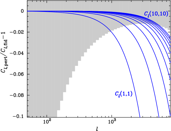
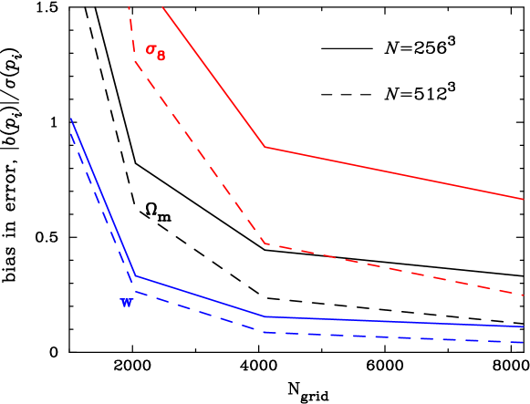
Figure 2: The top panel shows fractional differences between the lensing power spectra with and without the model biases in $P(k)$ due to finite size and resolution of the simulation, à la Eq. (7). The solid curves show the auto spectra of 10 redshift bin tomography, where the redshift bins are equally spaced between $z=0$ and $z=3$ and we assumed the simulation parameters of $L=200$ Mpc$/h$, $n=512^{3}$, and $N_{\rm grid}=4096$. The shaded region shows the $1\sigma$ statistical error for measuring the 5th redshift bin spectrum, $C_{55}^{\kappa}$, for the SNAP-type survey (1000 deg², 100 gal/arcmin² and $\langle\gamma_{\rm int}\rangle=0.22$). Bandwidth of $\Delta\ell/\ell\approx 0.11$ is assumed. The bottom panel shows how the bias in $P(k)$ propagates into the bias in cosmological parameters. We plot the bias in the cosmological parameters relative to their marginalized error vs. the ray-tracing simulation grid number $N_{\rm grid}$. The solid and dashed curves show the results for the two cases of N-body simulation particle number, $N=256^{3}$ and $N=512^{3}$, while the N-body simulation box size is fixed to $200$ Mpc$/h$.

The top panel of Figure 2 shows the fractional differences between the convergence power spectra with and without the model numerical error in $P(k)$. We assumed simulation parameters of $L_{\rm box}=200$Mpc$/h$, $N=512^{3}$ and $N_{\rm grid}=4096$, and in this case the term including $\sigma_{n}$ in Eq. (7) which models the finite force resolution in the N-body simulation provides dominant contribution to the error in $P(k)$ (also see Figure 3 in White & Vale 2004). We find that the model error in $P(k)$ causes the suppression of the lensing power spectrum amplitudes by $\lower 2.15277pt\hbox{$\;\buildrel<\over{\sim}\;$}10\%$ for $\ell\leq 3000$. Since a given angular mode $\ell$ corresponds to smaller $k$ as redshift increases, the lensing spectra of higher redshift bins arise from density perturbations of smaller $k$ and are therefore less affected by the numerical effects. The shaded region shows the 1$\sigma$ statistical error in the lensing spectrum measurement for the fiducial survey, where the error arises mainly from the cosmic sample variance at $\ell\lower 2.15277pt\hbox{$\;\buildrel<\over{\sim}\;$}10^{3}$, while the shot noise due to the intrinsic ellipticities is dominant at larger $\ell$. The departures in the lensing spectra of low redshift bins are larger than the statistical errors even though we only consider the measurements at $\ell\leq 3000$.

Thus, it is important to investigate how the numerical inaccuracy in $P(k)$ propagates into the biases in cosmological parameters, and we address this in the bottom panel of Figure 2. As with the statistical error in $P(k)$ (see Figure 1), the biases in $P(k)$ lead to a larger bias in $\sigma_{8}$ than those in $\Omega_{\rm m}$ and $w$. It is reassuring to see that the simulations with $N_{\rm grid}\geq 4096$ and $N=512^{3}$, which are feasible with current numerical resources, lead to the bias in $w$ and $\Omega_{\rm m}$ of less than about 20% relative to the marginalized error. Moreover, in the future one can expect to be able to calibrate, and partly correct for, the remaining bias in simulations by using a small number of even higher resolution simulations as a reference.

The effect of baryons on the non-linear mass clustering is another potentially harmful systematic effect on $P(k)$ (White 2004, Zhan & Knox 2004) and its calibration requires hydrodynamical N-body simulations that include baryon dissipation. Baryons, which constitute more than 10% of the total mass, cool and condense within a halo, and their effects are most pronounced for halos of mass $\lower 2.15277pt\hbox{$\;\buildrel<\over{\sim}\;$}10^{13}M_{\odot}$ (White 2004). The $X$-ray observations indicate that the hot baryons are likely to have a smoother profile than dark matter. Zhan & Knox (2004) estimated the effect of hot baryons on the lensing power spectrum assuming an isothermal $\beta$-model to describe the density profile of the baryon within the host halo. Their fiducial model leads to modifications in the lensing power spectrum of a few percent around $\ell\approx 10^{3}$ for source redshift $z=1$ (see Figure 2 in their paper). This effect is of similar amplitude as that shown in Figure 2, suggesting that the presence of hot baryons does not necessarily lead to drastic biases in the cosmological parameters. However, a much more extensive investigation that uses a suite of hydrodynamical simulations is needed to properly assess the effect of baryons on cosmological parameter estimation.

3.2 Worst-case Systematic Bias in $P(k)$

The most damaging systematic error in calibrating $P(k)$ will generally be error that mimics the behavior of cosmological parameters. Somewhat confusingly, however, the worst-case biased $P(k)$ (call it $Q(k)$) is typically not the matter power spectrum for some neighboring values of cosmological parameters. For, $Q(k)$ is weighted with the geometric factor to produce the observable convergence power spectrum, and the geometric factor is known exactly (provided that the redshift distribution of galaxies is known). Instead, the worst-case $Q(k)$ will be such that, when weighted by the geometric factor of the true cosmological model, it produces the convergence power spectrum which precisely matches some neighboring cosmological model.

While finding the actual worst-case $Q(k)$ is a thorny problem, we can compute the desired results in the approximation that the perturbation in $P(k)$ is small. The assumed deviation in the convergence power spectra is solely due to the bias in the matter power spectrum

$$C_{\alpha}^{\kappa}(\ell)-\bar{C}_{\alpha}^{\kappa}(\ell)=\sum_{a=1}^{N}\tilde{W}(k_{a})\,\delta P(k_{a}),$$ (8)

where we have discretized the integral as the sum over $N$ lens planes, or equivalently over $N$ values of the wavenumber $k=\ell/r(z)$, and defined $\tilde{W}(k)$ appropriately; c.f. Eq. (1). Then Eq. (6) can be rewritten as

$$\delta p_{i}=\sum_{a=1}^{N}(\delta\ln P(k_{a}))\,c_{a}^{(i)},$$ (9)

where we defined

$$c_{a}^{(i)}\equiv F_{ij}^{-1}\sum_{\ell}P(k_{a})\,\tilde{W}_{\alpha}(k_{a})\,{\rm Cov}^{-1}\left[\bar{C}^{\kappa}_{\alpha}(\ell),\bar{C}^{\kappa}_{\beta}(\ell)\right]\,{\partial\bar{C}_{\beta}^{\kappa}(\ell)\over\partial p_{j}},$$ (10)

where the summation over $j$, $\alpha$ and $\beta$ is implied. Let us assume for a moment that the bias in $\ln P(k)$ is known to be smaller, by absolute value, than some fixed number $\delta\ln P$. Then Eq. (9) shows that the worst-case bias in $P(k)$ – one that maximizes $\delta p_{i}$ – takes the value $\pm(\delta\ln P)$ on each lens plane, with the sign equal to the sign of $c^{(i)}$ on that plane. The resulting worst-case bias in the cosmological parameter is $\delta p_{i}=(\delta\ln P)\sum_{a=1}^{N}|c_{a}^{(i)}|$.

Turning the argument around, if the bias in a given cosmological parameter $p_{i}$ is to be smaller than $\delta p_{i}$, it is sufficient to trust the matter power spectrum to an accuracy better than

$$\delta\ln P={\delta p_{i}\over\sum_{a=1}^{N}\,|c_{a}^{(i)}|},$$ (11)

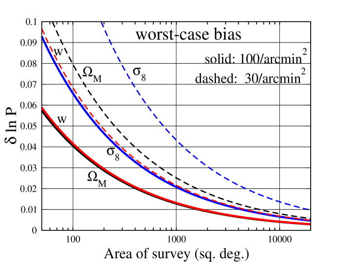
Figure 3: The necessary accuracy in $P(k)$ for the worst-case scenario of bias in $P(k)$, defined so that it produces the maximal bias in the three cosmological parameters shown. The required accuracy, plotted as a function of the sky coverage of the survey, is defined so that it limits the biases in the cosmological parameters to be no larger than their 1$\sigma$ fiducial accuracies. We show the cases of $n_{g}=100$ and $30$ gal/arcmin²

and this is true irrespective of the conspiring shape of $\delta\ln P(k)$. Figure 3 shows the required accuracy in $P(k)$, $\delta\ln P$, assuming the worst-case scenario where the bias equals the 1$\sigma$ accuracy in $p_{i}$. The required accuracy is shown as a function of area of the survey for two values of the density of galaxies (100 and 30 galaxies/arcmin²) and for three cosmological parameters that are of greatest interest to us ($\Omega_{M}$, $\sigma_{8}$ and $w$). As before, we find that more ambitious surveys have more stringent requirements on the systematic control of $P(k)$. We find that, in order for the worst-case systematics to be subdominant to the 1$\sigma$ error bars in the three cosmological parameters, a survey like SNAP will need a 1% calibration in $P(k)$ over the relevant scales, while LSST needs a better than 0.5% calibration. We emphasize that these are the required sensitivities for the worst-case scenario of bias in $P(k)$, where the bias in $P(k)$ conspires to introduce the maximal bias in the cosmological parameters. Section 2 shows that a more common error in $P(k)$ that is uncorrelated with cosmological parameters produces biases that are a factor of a few smaller.

4 Conclusions

Accurate knowledge of the full nonlinear matter power spectrum is crucial for the future weak gravitational lensing surveys to achieve their full potential. In this paper we have explored the required accuracy in $P(k,z)$ so that it does not bias the cosmological parameter extraction from future wide-field surveys. This analysis complements other analyses of theoretical and observational systematics in weak lensing measurements (e.g. Vale et al. 2004, Huterer et al. 2004).

We find that the power spectrum sensitivity is greatest at two decades in wavenumber centered around $k=1$ Mpc$/h$ comoving. Calibration of $P(k)$ on those scales needs to be better than a few percent ($\approx 2\%$ for $\sigma_{8}$ and 5-10% for $\Omega_{M}$ and $w$) for the SNAP-type experiment, and about a factor of two more stringent for the LSST-type experiment. We also consider the systematic biases in the power spectrum in N-body simulations. While the simulations’ accuracy is already nearly sufficient, the cooling and collapse of baryons, and even the clustering of massive neutrinos (Abazajian et al. 2004) may lead to large errors if they are not modeled accurately. There exist a number of options to protect against such effects (Huterer & White 2004), but exploring those is beyond the scope of this work. The most stringent accuracy requirement on $P(k)$ is obtained for the worst-case scenario where the bias in $P(k)$ conspires to produce the convergence power spectrum that is precisely reproduced by cosmological parameters with biased values. Fortunately, we find that even this worst-case scenario leads to tolerable biases in the cosmological parameters provided $P(k)$ is calibrated to 0.5-1% accuracy over the relevant scales. Note too that, in order to achieve $\sim 1$% accuracy in $P(k)$, current analytic fits for the linear power spectrum are not accurate enough either, and one instead needs to numerically solve the coupled Einstein, fluid and Boltzmann equations as done e.g. in the CMBFAST code (Seljak & Zaldarriaga 1996).

As we are entering the era of powerful wide-field WL surveys, currently popular fitting formulae for the power spectrum will soon become inadequate and one will need to resort to a full suite of N-body simulations, interpolating on a grid of cosmological models. First steps in such an approach were recently undertaken (White & Vale 2004) although many details remain to be worked out. We have shown here that the required accuracy is nearly within reach with current simulations, although the number of models that are necessary to be run might be very large. With the effort of the weak lensing community and ever-more powerful computers, the necessary simulation results should be in hand by the end of the decade, enabling weak lensing to realize its full power as a probe of dark energy and matter distribution in the universe.

DH is supported by the NSF Astronomy and Astrophysics Postdoctoral Fellowship. We thank Kev Abazajian, Gary Bernstein, Salman Habib, Bhuvnesh Jain, Lloyd Knox, Eric Linder, Chris Vale and Martin White for useful conversations.

References

- (1) Abazajian, K., Switzer, E.R., Dodelson, S., Heitmann, K., & Habib, S., astro-ph/0411552
- (2) Aldering, G. et al. 2004, PASP, submitted (astro-ph/0405232)
- (3) Bartelmann, M. & Schneider, P. 2001, Phys. Rep., 340, 291
- (4) Eisenstein, D.J. & Hu, W. 1999, ApJ, 511, 5
- (5) Heitmann, K., Ricker, P. M., Warren, M. S., Habib, S., 2004, astro-ph/0411795
- (6) Hu, W. 1999, ApJ, 522, L21
- (7) Hu, W. 2003, Phys. Rev. D, 66, 083515
- (8) Huterer, D., 2002, Phys. Rev. D, 65, 063001
- (9) Huterer, D. & Starkman, G. 2002, Phys. Rev. Lett., 90, 031301
- (10) Huterer, D., Takada, M. Bernstein, G. & Jain, B. 2004, astro-ph/0506030
- (11) Huterer, D., & White, M. 2004, Phys. Rev. D. (submitted), astro-ph/0501451
- (12) Ishak, M., Hirata, C.M., McDonald, P. & Seljak, U. 2004, Phys. Rev. D, 69, 083514
- (13) Jain, B., Seljak, U., ApJ, 1997, 484, 560
- (14) Jain, B., Seljak, U., White, S. D. M., 2000, ApJ, 530, 547
- (15) Jenkins, A. R. et al. 2001, MNRAS, 321, 372
- (16) Ma, C.-P., Caldwell, R. R., Bode, P., & Wang, L. 1999, ApJ, 521, L1
- (17) Ma, Z., Hu, W. & Huterer, D. 2004, in preparation
- (18) Refregier, A. 2003, Ann. Rev. Astron. Astrophys., 41, 645
- (19) Refregier, A. et al. 2003, MNRAS, 346, 573
- (20) Seljak, U. & Zaldarriaga, M. 1996, ApJ, 469, 437
- (21) Smith, R.E. et al. 2003, MNRAS, 341, 1311
- (22) Song, Y.-S. & Knox L. 2004, Phys. Rev. D, 70, 063510
- (23) Takada, M. & Jain, B. 2004, MNRAS, 348, 897
- (24) Takada, M. & White, M. 2004, ApJ, 601, L1
- (25) Vale, C. & White, M., 2003, ApJ, 592, 699
- (26) Vale, C., Hoekstra, H., van Waerbeke, L. & White, M. 2004, ApJ, 613, L1
- (27) Van Waerbeke, L., Mellier, Y., 2003, astro-ph/0305089
- (28) White, M., 2004, Astroparticle. Phys., 22, 211
- (29) White, M. & Hu, W., 2000, ApJ, 537, 1
- (30) White, M. & Vale, C., 2004, Astroparticle. Phys., 22, 19
- (31) Zhan, H. & Knox, L. 2004, ApJ, 616, L75