Growth of primordial black holes in a universe containing a massless scalar field

Abstract

The evolution of primordial black holes in a flat Friedmann universe with a massless scalar field is investigated in fully general relativistic numerical relativity. A primordial black hole is expected to form with a scale comparable to the cosmological apparent horizon, in which case it may go through an initial phase with significant accretion. However, if it is very close to the cosmological apparent horizon size, the accretion is suppressed due to general relativistic effects. In any case, it soon gets smaller than the cosmological horizon and thereafter it can be approximated as an isolated vacuum solution with decaying mass accretion. In this situation the dynamical and inhomogeneous scalar field is typically equivalent to a perfect fluid with a stiff equation of state $p=\rho$. The black hole mass never increases by more than a factor of two, despite recent claims that primordial black holes might grow substantially through accreting quintessence. It is found that the gravitational memory scenario, proposed for primordial black holes in Brans-Dicke and scalar-tensor theories of gravity, is highly unphysical.

I Introduction

The observed anisotropy and polarisation of the cosmic microwave background radiation give very precise information about the cosmic history since last scattering. Using a simple physical model, we can determine cosmological parameters with very high accuracy and also learn about structure formation and reionisation. Nevertheless, it is still difficult to obtain information about the universe before big bang nucleosynthesis without making many extra assumptions. In this context, primordial black holes (PBHs) could be one of the most important fossils of the very early universe. Such black holes may have formed directly from primordial density perturbations hawking1971a and may contribute to the cosmological $\gamma$-ray background radiation, the cosmic ray flux and the dark matter density. This leads to important observational constraints on the number of PBHs carr1975 and hence on models of the very early universe.

To understand these constraints, it is important to know whether PBHs can accrete enough to become much more massive than they were at formation. This topic has a long history. It was originally claimed, on the basis of a simple Newtonian argument, that a PBH much smaller than the cosmological particle horizon at formation would not accrete much at all, whereas one comparable to the horizon size would continue to grow at the same rate as the horizon until the end of the radiation-dominated era zn1967 . Since one would expect a PBH to be of order the particle horizon size at formation in order to collapse against the pressure, this suggests that all PBHs might grow to the horizon mass at the end of the radiation era, which is about $10^{15}$ solar masses. Since there is no evidence for such enormous black holes in the universe today, the conclusion seemed to be that PBHs never formed.

However, this conclusion was very suspect. If PBHs really could grow as fast as the particle horizon, there would have to exist spherically symmetric self-similar solutions to Einstein’s equations containing black holes in an exact Friedmann background. A study of solutions of this kind containing radiation (i.e. fluid with equation of state $p=\rho/3$) showed that there are no self-similar PBH solutions if the black hole is formed by purely local processes (i.e. if the background is exactly Friedmann beyond some radius). Self-similar solutions are possible only if the initial perturbation of the Friedmann background extends to infinity ch1974 . Since the PBH must soon become much smaller than the cosmological horizon, at which point the Newtonian argument should be applicable, this suggests that it will only increase its mass by a small amount.

This conclusion was subsequently extended to more general fluids, with an equation of state of the form $p=k\rho$ carr1976 ; bh1978a . Although there was an initial claim that self-similar growth might be possible in the special case of a stiff fluid ($p=\rho$) lcf1976 , this claim was subsequently challenged bh1978b . It was found to be true only in rather contrived circumstances in which the stiff fluid is converted into radiation at the black hole’s event horizon. Therefore the conclusion that there are no self-similar solutions containing PBHs formed by purely local processes seems to be true very generally. See cc2000 for a review of self-similar solutions. This conclusion is also confirmed by numerical calculations. If the formation and evolution of a PBH in a general fluid universe with a local perturbation is simulated numerically, without assuming self-similarity, it is found that the PBH soon becomes much smaller than the cosmological horizon and this excludes self-similar growth nnp1978 ; np1980 . More recently, PBH formation from density perturbations has been investigated in the context of critical phenomena nj1999 ; jn1999 ; ss1999 ; hs2002 ; mmr but again with no evidence for self-similar growth.

Hitherto studies of PBHs have mainly focused on perfect fluid universes with equation of state $p=k\rho$. However, it is also natural to consider a universe whose density is dominated by a scalar field. For example, in the chaotic inflation scenario it is postulated that there is a pre-inflationary stage in which the scalar field moves randomly in space and time. In the pre-heating inflationary scenario, it is also natural to consider a scalar-field-dominated era kls1994 . More recently, the study of PBHs in the quintessence scenario has attracted attention frol2004 . It is therefore important to examine whether the conclusion that PBH accretion is small also applies in this case.

If the scalar field is massless and there is no scalar potential, then it is well known madsen1988 that it is equivalent to a stiff fluid providing the gradient of the scalar field remains timelike, as usually applies. The fact that there is no self-similar solution in the stiff case therefore suggests that accretion is also limited in the scalar field case. Despite this, the original Newtonian argument for self-similar growth has recently been applied in the quintessence scenario to argue that PBHs could grow enough to form the supermassive black holes found in galactic nuclei bm2003 . A generalization of this analysis ch2005 , not necessarily involving self-similarity but still based on the Newtonian analysis, has also claimed there could be appreciable quintessence accretion in some circumstances. Both these analyses contravene the conclusions of the earlier work discussed above. However, since the earlier work did not strictly include the scalar field case and did not allow for a scalar potential, a more careful analysis is required before concluding that these analyses are erroneous.

Scalar fields are also relevant in Brans-Dicke and scalar-tensor theories of gravity, where the gravitational “constant” varies in space and time. This is because, if there is a single gravitational scalar field, such theories can be transformed into the usual Einstein gravity with a single scalar field de1992 . Brans-Dicke and scalar-tensor theories are particularly relevant to PBHs since the black holes may form when $G$ was very different from today. Indeed the “gravitational memory” scenario has been proposed barrow1992 , in which the value of $G$ within the black hole is assumed to be preserved as the cosmological background value evolves. The observational constraints on PBHs depend strongly on whether or not one has gravitational memory bc1996 . It is not clear whether this applies but, if it does, it should be due to the properties of the black hole event horizon rather than those of the matter fields involved.

It is interesting that the problem of gravitational memory is also closely related to the problem of accretion cg1999 . This is because it turns out that appreciable accretion of the scalar field energy is required for gravitational memory to be preserved and so the issue of whether there is a self-similar solution again becomes relevant. Indeed Carr and Goymer argued that there is unlikely to be gravitational memory on the grounds that there is no self-similar solution in the stiff fluid case cg1999 . Evidence against the gravitational memory scenario, at least in particular situations, has also been obtained using other arguments jacobson1999 ; hgc2002 .

As a first step to investigating these questions numerically, in this paper we consider a universe containing a massless scalar field but no matter. To implement the simulations, we use a double-null formulation of the Einstein equations based on the work by Hamadé and Stewart hs1996 . This has been shown to be a very powerful tool for investigating critical collapse hs1996 and the internal structure of black holes sp1999 . This study represents an improvement on earlier work hgc2002 , in which the gravitational effect of the scalar field was neglected, since it uses the full field equations. It should also be seen in conjunction with two other papers hc2004a ; hc2004b ; we consider general constraints on the size of a PBH at formation in the first and some effects associated with very large PBHs in the second.

The plan of the paper is as follows. In Section II, we describe the double-null formulation and present the basic equations for the scalar field case. In Section III, we discuss how we set up the initial data for the simulations. Section IV presents our results, with particular emphasis on the evolution of the black hole event horizon and the spatial profile of the scalar field. In Section V, we discuss the implications of these results for the accretion and gravitational memory issues, also considering the applicability of the Newtonian accretion formula. In Section VI, we draw some general conclusions. Details of the numerical code and particular exact solutions are described in Appendices. We adopt units in which $G=c=1$ and the abstract index notation of reference wald1983 .

II Double-null formulation of the Einstein equations

We consider a massless scalar field in general relativity, for which the stress-energy tensor is

$$T_{ab}=\Psi_{,a}\Psi_{,b}-\frac{1}{2}g_{ab}\Psi^{,c}\Psi_{,c}.$$ (1)

The Einstein equations are

$$R_{ab}-\frac{1}{2}g_{ab}R=8\pi T_{ab},$$ (2)

and the equation of motion for the scalar field is

$$\Box\Psi=\Psi^{;a}_{~{}~{};a}=0.$$ (3)

We also focus on a spherically symmetric system, for which the line element can be written in the form

$$ds^{2}=-a^{2}(u,v)dudv+r^{2}(u,v)(d\theta^{2}+\sin^{2}\theta d\phi^{2}),$$ (4)

where $u$ and $v$ are advanced and retarded time coordinates, respectively, and $r$ is the “area radius” (the proper area of the sphere of constant $r$ being $4\pi r^{2}$). Eqs. (2) and (3) then imply that we have 14 first-order partial differential equations and two auxiliary equations (see Section 2 of hs1996 ). By adopting a double-null coordinate choice, we can simulate regions outside the cosmological apparent horizon and inside the black hole apparent horizon simultaneously.

In spherically symmetric spacetimes the existence and position of apparent horizons can be inferred from the form of the Hawking mass. This is a well-behaved quasi-local mass, which can be written as

$$m=\frac{r}{2}\left(1+\frac{4r_{,u}r_{,v}}{a^{2}}\right).$$ (5)

Using the above equation and Eq. (2.6) of hs1996 , we can derive the following useful relations:

$$m_{,u} = -\frac{8\pi r^{2}r_{,v}(\Psi_{,u})^{2}}{a^{2}},$$ (6)

$$m_{,v} = -\frac{8\pi r^{2}r_{,u}(\Psi_{,v})^{2}}{a^{2}}.$$ (7)

A region is trapped if $r_{,u}<0$ and $r_{,v}<0$, while it is antitrapped if $r_{,u}>0$ and $r_{,v}>0$. The black hole and cosmological apparent horizons are defined as marginally trapped and anti-trapped surfaces, respectively. Providing the black hole horizon is within the cosmological horizon, these correspond to the conditions $r_{,v}=0$ and $r_{,u}=0$, respectively. Thus the relation $r=2m$ is satisfied on both apparent horizons because $r_{,u}r_{,v}=0$ there. We confine attention to this situation in the present paper. However, as discussed in a separate paper hc2004b , in some circumstances the black hole horizon can be outside the cosmological horizon and the situation is then more complicated. In this case, we can still use two different marginal surfaces on which $r_{,v}=0$ and $r_{,u}=0$, respectively hayward1996 . However, these are no longer everywhere identified with the black hole and cosmological apparent horizons.

Note that the black hole and cosmological apparent horizons are distinct from the black hole event horizon and cosmological particle horizon, which are always null. For numerical purposes, the apparent horizons are easier to find than the event and particle horizons because the complete spacetime, including the initial singularity, is needed to identify the latter, whereas the former can be found from the quasi-local properties of spacetime alone. However, we will also discuss the behaviour of the black hole event horizon in Section IV.

We first consider the flat Friedmann model, for which $a^{2}(u,v)$, $r(u,v)$ and $m(u,v)$ are given explicitly in terms of the standard double null coordinates in Appendix B. The condition $r=2m$ implies that the cosmological apparent horizon is $3u+v=0$ and this implies that its radius is just the Hubble scale $H^{-1}$ in a flat Friedmann universe, as described in hc2004a . On the other hand, the cosmological particle horizon is clearly $u=0$, corresponding to a photon propagating outwards from the big bang. This implies that the apparent horizon is always outside the particle horizon and the conformal diagram of the spacetime is as indicated in Fig. 1. This also shows the initial (big bang) spacelike singularity. If one perturbs such a spacetime but without introducing a black hole, the conformal diagram remains the same but the trajectories of constant space and time coordinate change. If one has a black hole embedded in an exact or asymptotically flat Friedmann model, the conformal diagram will change to the form indicated in Fig. 2. There are now also a black hole event horizon and apparent horizon, although one cannot give explicit analytic expressions for these, and a final (black hole) spacelike singularity.

If we define time and space coordinates, $T$ and $X$, by

$$u = T-X,$$ (8)

$$v = T+X,$$ (9)

we can put the 2-dimensional part of the metric tensor into conformally flat form. As in the usual 3+1 approach, we define the energy density $\rho_{\rm H}$ and momentum density $J$ measured by an observer moving normal to the $T=\mbox{const}$ spacelike hypersurface by

$$\rho_{\rm H} \equiv T_{ab}\hat{T}^{a}\hat{T}^{b},$$ (10)

$$J \equiv -T_{ab}\hat{T}^{a}\hat{X}^{b},$$ (11)

where $\hat{T}^{a}$ and $\hat{X}^{b}$ are unit vectors parallel to $T^{a}$ and $X^{b}$, respectively.

It should be stressed that the above description is observer-dependent and one can adopt another point of view. Providing the scalar field is vorticity-free and has a timelike gradient, it is equivalent to a perfect fluid with a “stiff” equation of state $p=\rho$ madsen1988 . The stress-energy tensor is then

$$T^{ab}=\rho_{\rm S}(g^{ab}+2U^{a}U^{b}),$$ (12)

where the energy density $\rho_{\rm S}$ and the 4-velocity $U^{a}$ of the stiff fluid are

$$\rho_{\rm S} = -\frac{1}{2}\Psi_{,a}\Psi^{,a},$$ (13)

$$U_{a} = \frac{-\Psi_{,a}}{\sqrt{-\Psi^{,b}\Psi_{,b}}}.$$ (14)

It should be noted that the 4-velocity of the stiff fluid is parallel to the (timelike) gradient of the scalar field. We can define an observer-independent velocity function by

$$V\equiv\frac{dr}{d\tau}=r_{,a}U^{a},$$ (15)

this being the rate of increase of $r$ per unit proper time $\tau$ along the worldline of the equivalent stiff fluid element. Appendix A gives expressions for these physical quantities in terms of the quantities calculated numerically.

III Initial data for PBHs

III.1 Structure of initial data

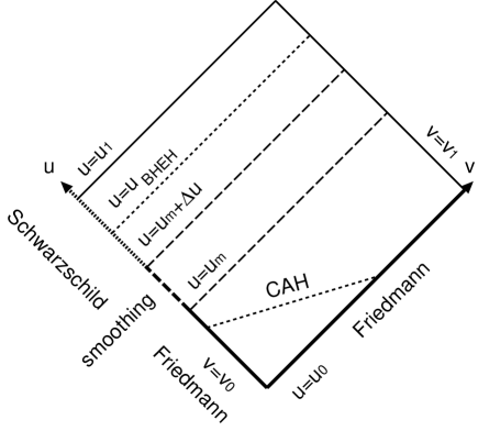
Figure 3: Schematics figure of the initial data setting. The relation between $u_{m}$ and CAH is true only for Models A-C.

The initial data are prescribed on the outgoing null surface $u=u_{0}$ and the ingoing null surface $v=v_{0}$. The region of calculation is the diamond $[u_{0},u_{1}]\times[v_{0},v_{1}]$ shown in Fig. 3, which is also equivalent to the diamond in Fig. 2. We have three independent functions on the two null surfaces: $a^{2}$, $\Psi$ and $r$. Two of them can be chosen freely and the other one is determined by the initial value equations on the null surfaces. It is convenient to choose

$$a^{2}(u_{0},v),a^{2}(u,v_{0}),\Psi(u_{0},v),\Psi(u,v_{0})$$ (16)

as the free initial data and to regard

$$r(u_{0},v),r(u,v_{0})$$ (17)

as being determined by the initial value equations. We can regard $\Psi(u_{0},v)$ and $\Psi(u,v_{0})$ as the physical degrees of freedom in the initial data, while the choice for $a^{2}(u_{0},v)$ and $a^{2}(u,v_{0})$ fixes the gauge.

It is usually assumed that the perturbation from which the PBH forms is local, so that the universe is exactly Friedmann at sufficiently large distances. Since information propagates at the speed of light, the matching between the perturbed and flat Friedmann regions always corresponds to some outgoing null ray $u=u_{\rm m}=\mbox{const}$ and such a ray is shown in Fig. 3. This means that the region outside the matching surface $u=u_{\rm m}$ is always described by the flat Friedmann solution. On the outgoing null surface $u=u_{0}$, we therefore assume that the initial data are given by the flat Friedmann solution for $v_{0}\leq v\leq v_{1}$. On the ingoing null surface $v=v_{0}$, we assume they are given by the flat Friedmann solution for $u_{0}\leq u<u_{\rm m}$ but by some perturbation of it for $u_{\rm m}\leq u\leq u_{1}$, where an appropriate matching is implemented at $u=u_{\rm m}$. As described in the next section, the perturbed region contains a Schwarzschild black hole. However, since this is a vacuum solution, it only applies instantaneously at $v=v_{0}$ because the inflowing matter will fill the vacuum immediately.

If the perturbation is assumed to be local, we can derive various upper limits on the black hole size hc2004a . These are generally within the cosmological particle horizon, which would then correspond to the line $u=0$ in Fig. 3. However, a perturbation can be larger than the cosmological particle horizon in some circumstances – indeed most of the cases we consider in this paper have this feature. The particle horizon is then within the perturbed region and no longer given by $u=0$. In some circumstances, e.g. for quantum fluctuations resulting from inflation, the perturbation may extend indefinitely, or at least well beyond the usual particle horizon. Generally the only upper limit on the size of the perturbation comes from the requirement that the the perturbed region must be part of our universe rather a separate closed universe. The condition for this has been derived precisely for the situation in which the collapsing region is homogeneous and the equation of state is $p=k\rho$ hc2004a . In this case, the closed-universe scale is always well beyond the cosmological apparent horizon size. Even if the perturbed region is within our universe, the solution may exhibit anomalous features if it is too large. These anomalies are described elsewhere hc2004b but we do not choose initial data which lead them to arise in this paper.

III.2 Setting up the initial data

In the flat Friedmann region, we choose the coordinate system given in Appendix B.1. We also impose flat Friedmann initial data for $a^{2}$ and $\Psi$ on the initial outgoing null surface $u=u_{0}$ with $v_{0}\leq v\leq v_{1}$. This is also given in Appendix B.1. On the initial ingoing null surface $v=v_{0}$, we choose flat Friedmann data for $a^{2}$ for $u_{0}\leq u\leq u_{1}$. For the function $\Psi$, we use the same data on the initial ingoing null surface for $u_{0}\leq u\leq u_{\rm m}$, but $\Psi=\mbox{const}$ for $u_{\rm m}+\Delta u<u\leq u_{1}$. This is equivalent to Schwarzschild data in coordinates penetrating the black hole (cf. Appendix B.2). The sudden transition from flat Friedmann data to Schwarzschild data results in a discontinuity at $u=u_{\rm m}$, which reduces the numerical accuracy. Hence we smooth the transition with some smoothing length $\Delta u$; we use a quadratic function between $u_{\rm m}$ and $u_{\rm m}+\Delta u$, so that $\Psi$ and $\Psi_{,u}$ are continuous. More precisely, we impose the following initial data for $a^{2}$ and $s\equiv\sqrt{4\pi}\Psi$:

$$a^{2}(u,v_{0}) = C^{2}\left(\frac{u+v_{0}}{2}\right),$$ (18)

$$s(u,v_{0}) = \left\{\begin{array}[]{ll}\displaystyle\frac{\sqrt{3}}{2}\ln\left(\displaystyle\frac{u+v_{0}}{2}\right)+s_{0}&\quad(u<u_{\rm m})\\ \displaystyle\frac{\sqrt{3}}{2}\left[\displaystyle\frac{(\Delta u)^{2}-(u_{\rm m}+\Delta u-u)^{2}}{2\Delta u(u_{\rm m}+\Delta u)}+\ln\left(\displaystyle\frac{u_{\rm m}+v_{0}}{2}\right)\right]+s_{0}&\quad(u_{\rm m}\leq u<u_{\rm m}+\Delta u)\\ \displaystyle\frac{\sqrt{3}}{2}\left[\displaystyle\frac{\Delta u}{2(u_{\rm m}+v_{0})}+\ln\left(\displaystyle\frac{u_{\rm m}+v_{0}}{2}\right)\right]+s_{0}&\quad(u\geq u_{\rm m}+\Delta u)\end{array}\right.,$$ (22)

on the initial ingoing null surface $v=v_{0}$, and

$$a^{2}(u_{0},v) = C^{2}\left(\frac{u_{0}+v}{2}\right),$$ (23)

$$s(u_{0},v) = \frac{\sqrt{3}}{2}\ln\left(\frac{u_{0}+v}{2}\right)+s_{0},$$ (24)

on the initial outgoing null surface $u=u_{0}$. Here $C$ and $s_{0}$ are constants and, without loss of generality, we can choose $C=1$ and $s_{0}=0$. Note that one has a Schwarzschild vacuum for $u\geq u_{\rm m}+\Delta u$. However, as noted above, this situation only applies instantaneously at $v=v_{0}$, since the vacuum will be filled with the scalar field at any later or earlier time. Nevertheless, one expects the event horizon to evolve smoothly, so it will still be described by a single null line, as illustrated qualitatively in Fig. 3

To summarise, two parameters describe the initial conditions: the location of the matching surface and the smoothing length. The region outside the matching surface is the exact flat Friedmann solution, so the first parameter determines the mass of the perturbed region. The second parameter determines the mass of the black hole compared to the perturbed mass. A small smoothing length means a narrow boundary between the exterior Friedmann region and the interior vacuum region. In this case, the mass inside the vacuum region is nearly the same as that within the matching surface and so a large mass is concentrated at the central singularity. A large smoothing length means a wide boundary, so the mass inside the vacuum region is much smaller than this and so a small mass is concentrated at the central singularity. For vanishing smoothing length, the black hole mass would be the same as that at the matching surface, so $u_{m}$ would also be the black hole event horizon, although it is difficult to implement this numerically because of the strong discontinuity.

IV Results

The numerical code is based on Hamadé and Stewart hs1996 , although it is slightly modified so as to be accurate to second-order (see Appendix A). As indicated in Fig. 3, the calculated region is the diamond contained by $u_{0}$, $v_{0}$, $u_{1}$ and $v_{1}$. The initial data are prescribed on the ingoing null surface $v_{0}=1$ and the outgoing null surface $u_{0}=-0.5$. The values $u_{0}$ and $v_{0}$ fix the units. For example, the background value for the Hubble parameter at $(u_{0},v_{0})$ is 4 and the Hubble length becomes 0.25 from Eq. (66). The value of $u_{1}$ is always taken to be 1.1 but $v_{1}$ varies between 2 and 4. On the initial ingoing null surface, we make the matching at three values of $u_{\rm m}$ in the range $-0.5$ to 0. We also use small and large smoothing lengths, corresponding to $\Delta u=0.02$ and $\Delta u=0.5$, respectively.

As shown in Appendix B.1, the cosmological apparent and particle horizons are given by $u_{\rm CAH}=-v/3$ and $u_{\rm CPH}=0$, respectively, in the flat Friedmann model. As time proceeds, the outgoing null rays will become ever more sensitive to $r$ near the black hole event horizon, so the calculation is stopped at the value of $v$ at which the outgoing null rays near the black hole event horizon become too coarse to resolve. This then specifies the value $v_{1}$ in Fig. 3. As shown in Appendix B.1, the radius of the unperturbed cosmological apparent horizon and the mass within it are given by

$$m_{\rm CAH}=r_{\rm CAH}/2=Cv^{3/2}/(3\sqrt{3}).$$ (25)

However, this equation must be modified if the perturbed region extends beyond the usual cosmological apparent horizon and this applies in one of the cases considered.

The model parameters and initial black hole to cosmological horizon mass ratios are summarised in Table 1. We present results for four models. For Model A, a sharp matching is made at the cosmological apparent horizon. For Model B, a sharp matching is made at the cosmological particle horizon, which is well inside the cosmological apparent horizon. For Model C, a smooth matching is made at the cosmological apparent horizon. For Model D, a smooth matching is made well outside the cosmological apparent horizon, although the black hole itself is inside it. In a separate paper hc2004b , we consider models in which a sharp matching is made well outside the cosmological apparent horizon. These models have very different qualitative features, even the conformal diagram being modified, which is why we consider them separately.

IV.1 Black hole horizons

Figure 4 shows the locations of the black hole event horizon and apparent horizon and the cosmological apparent horizon in the $(u,v)$ plane for the four models. Each figure can be identified with the diamond in Fig. 3, tilted through 45 degrees. In all cases, it is seen that the black hole apparent horizon is initially well within the event horizon but approaches it as time proceeds. In Fig. 4(b), the location of the (unperturbed) cosmological particle horizon of the exact flat Friedmann solution is also plotted. In other cases, the cosmological particle horizon is perturbed, so we do not plot it. The cosmological apparent horizon is unperturbed except in case D.

The radii and masses of the black hole apparent horizon and event horizon for Models A–D are shown, together with those for the cosmological horizons, in Figs. 5 and 6. The initial and final values and their ratios are also summarised in Tables 2 and 3. All three horizons approximately coincide at $v=1$ for Model A, both in radius and mass, as seen in Figs. 5(a) and  6(a). Figs. 5 and  6 show that the qualitative features of the evolution for Models A–D are very similar. The radius of the cosmological apparent horizon of the unperturbed flat Friedmann solution grows like $v^{3/2}$, while the black hole apparent horizon and event horizon converge and grow much more slowly. As a consequence, the black hole horizons soon get much smaller than the cosmological apparent horizon. This is also the case for the corresponding masses.

Since the black hole event horizon is given by the curve $u=u_{\rm BHEH}=\mbox{const}$, Eq. (7) gives the mass accretion rate of the black hole. This also serves as a consistency check for numerical accuracy. The result for Models A–D is shown in Fig. 7, where both sides of Eq. (7) are plotted. We find that the curves are almost indistinguishable, which implies very good numerical accuracy. For Model A, the accretion rate starts very small, then increases, reaches a maximum of $0.0691$ at $v\simeq 1.75$ and then decreases to a very small value. Recall that the units are such that the background Hubble parameter is 4 and the background Hubble length is 0.25 at $u_{0}$ and $v_{0}$. For Models B and C, the accretion rate starts with its maximum value and then monotonically decreases. The features for Model D are similar to those for Model A.

An important qualitative feature is that accretion is suppressed for a PBH nearly as large as the cosmological apparent horizon. (In Model D the black hole event horizon happens to be close to the cosmological apparent horizon.) This is because Eq. (7) implies that the mass accretion rate is proportional to $(-r_{,u})$, i.e. the ingoing null contraction, and this vanishes at the cosmological apparent horizon. This feature is a purely general relativistic effect and there is no analogue in Newtonian gravity. It can be understood physically as arising because the scalar field must be partaking in the cosmic expansion at sufficiently large distances, rather than accreting onto the black hole. Since the sound speed is the speed of light for a scalar field, the cosmological apparent horizon is likely to be the transition point. A more rigorous explanation of this effect is presented in Section V, where it is shown to apply for more general fluids.

We conclude that, even if a PBH starts off as large as the cosmological apparent horizon, it soon gets considerably smaller than it. Whatever the initial size of the PBH, accretion can be large only for about a Hubble time, after which it becomes ineffective. As seen in Tables 2 and 3, the mass increase is at most 79 % for our models.

IV.2 Geometry and scalar field

Since the qualitative features of the numerical results are very similar for Models A–D, in this subsection we concentrate on Model A. Figure 8 shows the evolution of the area radius $r$ in terms of $u$ and $v$. We can see from Fig. 8(b) that there is a threshold value of $u$: outgoing null rays with smaller $u$ go to infinity, while those with larger $u$ go to the singularity at $r=0$. Therefore, this threshold value can be identified with the black hole event horizon $u_{\rm BHEH}\simeq 0.702$. Since $r_{,v}$ approaches zero along the black hole event horizon, all ingoing null rays seem to cross it at almost the same radius in Fig. 8(a). In fact, the integration is continued well beyond $v=v_{1}$ to locate the black hole event horizon accurately. Figure 8(b) shows that the radius of the black hole event horizon reaches $0.694$ at $v=4$ and this might be regarded as its asymptotic value.

Figure 9 shows the evolution of $2m/r$ in terms of $u$ and $v$. There is an apparent horizon where this is unity. The signs of both ingoing and outgoing null expansions are the same when this is larger than unity. A region is untrapped when it is smaller than unity. As seen in Fig. 9(a), $2m/r$ is almost exactly unity in the perturbed region at the initial ingoing null surface $v=v_{0}=1$. As $u$ increases, there then appears a black hole apparent horizon, beyond which the region is trapped. There is also a cosmological apparent horizon at $u=-1/3$ and $v=v_{0}=1$, although it goes outside the calculated region during the evolution. As time proceeds, the value of $2m/r$ in the untrapped region between the black hole and cosmological apparent horizons becomes smaller and the curve near the black hole apparent horizon becomes steeper. As seen in Fig. 9(b), there is no black hole apparent horizon before the event horizon forms at $u=u_{\rm BHEH}\simeq 0.702$. At $u=u_{\rm BHEH}$, $2m/r$ approaches unity from below as $v$ increases. Soon after $u=u_{\rm BHEH}$, a black hole apparent horizon appears.

Figure 10 shows the evolution of the scalar field for Model A. For clarity, it is plotted in terms of both $(v,r)$ and $(T,r)$ coordinates. In either case there is no coordinate singularity at the black hole horizons as the ingoing Eddington-Finkelstein coordinate is well-behaved for the Schwarzschild black hole. In the $(v,r)$ diagram of Fig. 10(a), the broken and solid light curves give the results of the simulations and the evolution of the flat Friedmann solution, respectively. Because of the initial perturbation, the value of the scalar field in the perturbed region starts off much smaller than that of the flat Friedmann solution. Thereafter, the perturbed scalar field tends to evolve as in the flat Friedmann solution. The position of the event horizon is shown by the solid heavy curve. Since the radius of the black hole event horizon is $0.694$ at $v=4$, the region inside the black hole event horizon is also calculated accurately. The evolution of the scalar field is well described by the flat Friedmann evolution with a small perturbation both outside and inside the black hole event horizon. The scalar field is smooth at the black hole event horizon. Fig. 10(b) shows the equivalent results in the $(T,r)$ diagram. It should be stressed, however, that there is no unique choice of spatial hypersurface and the profile of $\Psi$ would be different with another choice.

Figure 11 shows the energy density $\rho_{\rm H}$ and momentum density $J$ measured by the observer moving normal to the $T=\mbox{const}$ spacelike hypersurface for Model A. Since this normal observer coincides with the comoving observer in the flat Friedmann universe, $J$ vanishes in the flat Friedmann region for $u<u_{\rm m}$ (see Appendix B.1). In terms of the energy density $\rho_{\rm H}$, there is an underdense region inside the flat Friedmann region. Inside this underdense region, there is an overdense region around the black hole event horizon, where the energy density increases with time. In terms of the momentum density $J$, there is considerable energy infall around the black hole event horizon. $|J|$ increases significantly near the black hole event horizon, although we should note that this is an observer-dependent view.

Figure 12 shows the observer-independent quantities $\rho_{\rm S}$ and $V$. These are the energy density and velocity of the equivalent stiff fluid. The spikes correspond to the matching coordinate $u_{m}$. It is interesting that $\rho_{\rm S}$ is everywhere positive. This is a non-trivial result since $\rho_{\rm S}$ could in principle be negative if the spatial gradients were large enough. This is related to the fact, as illustrated in Fig. 12(a), that the gradient of the scalar field is always timelike in this simulation. (Otherwise it would not be equivalent to a stiff fluid.) Also, in terms of the density $\rho_{\rm S}$, we can see an underdense region just inside the flat Friedmann region. Within this underdense region, the energy density increases as one moves inwards. However, the energy density decreases nearly homogeneously for $v\geq 2.5$. In terms of the velocity $V$, the region near the black hole is infalling, as seen in Fig. 12(b), but the infall velocity profile near the black hole event horizon is almost stationary. We conclude that the growth of $\rho_{\rm H}$ and $|J|$ around the black hole event horizon is completely due to the Lorentz factor. Physically, the energy density $\rho_{\rm S}$ is slowly decreasing and the infall velocity profile $V$ is almost stationary near the black hole event horizon. These results suggest that the PBH can be regarded as almost isolated, with a relatively small mass accretion for $v\gtrsim 2$. This is consistent with the mass accretion rate seen in Fig. 7(a). Although there are apparent discontinuities at large radii in Figs. 11 and 12, this is only due to the narrow boundary and all quantities are continuous everywhere.

V Discussion

V.1 Self-similar growth and the Newtonian accretion formula

Various arguments zn1967 ; ch1974 ; cg1999 ; hc2004a lead to an estimate for the mass accretion rate of a PBH in a cosmological background of the form

$$\frac{dm_{\rm BH}}{dt}=4\pi\alpha\rho v_{\rm s}r_{\rm A}^{2}$$ (26)

where $\rho$ is the background density, $v_{\rm s}$ is the sound speed, $r_{\rm A}$ is the accretion radius of the hole and $\alpha$ is a dimensionless constant which depends on the equation of state ($p=k\rho$) and other features of the accretion flow. None of these arguments is precisely correct, since they all involve approximations which make them in some respects Newtonian. In particular, the value of $\alpha$ depends upon whether one allows for such effects as the relativistic sound speed, relativistic pressure and relativistic focussing. Also a stationary flow is usually assumed and the background cosmological expansion is neglected. Nevertheless it might be hoped that these inaccuracies could be absorbed into the constant $\alpha$.

If one assumes that the appropriate density to use in Eq. (26) is the background cosmological density $\sim 1/(Gt^{2})$, the accretion rate becomes

$$\frac{dm_{\rm BH}}{dt}=\frac{m_{\rm BH}^{2}}{\beta t^{2}},$$ (27)

where $\beta$ is another constant with units $c^{3}/G$. This has the following solution:

$$m_{\rm BH}=\frac{\beta t}{1+\frac{t}{t_{f}}\left(\frac{\beta t_{f}}{M_{f}}-1\right)}$$ (28)

where $M_{f}$ is the mass of the black hole when it forms at time $t_{f}$. If the hole is much smaller than the particle horizon at formation ($M_{f}\ll\beta t_{f}$), this implies that there is very little growth. However, if $M_{f}$ is chosen so that the term in brackets in Eq. (28) is zero, it suggests the possibility of self-similar growth with $m_{\rm BH}\propto t$. We assume the constant $\beta$ is $6$, since that is what the analysis of reference hc2004a implies when $k=1$. If the Newtonian formula were correct, the ratio would be order of unity. See hc2004a for a full discussion of the solutions.

In discussing the accretion rate for a scalar field, which is relevant here, one possibility is to regard it as a stiff fluid. In this case, one can apply the above analysis with $\beta$ having the value appropriate for $k=1$ and this is the approach used by Carr and Goymer cg1999 . Bean and Magueijo bm2003 also assume the accretion is given by Eq. (26) but identify $\rho$ with the kinetic energy of the scalar field  $(1/2)\dot{\Psi}^{2}$. However, since this is assumed to falls off as $1/t^{2}$, they obtain an equation of the same form as Carr and Goymer, though with a different constant since they allow for a scalar potential. Custodio and Horvath ch2005 allow for a broader range of behaviours for $\dot{\Psi}$, leading to a generalization of Eq.( 28). All of these analyses suggest that the black hole could grow self-similarly with a fine-tuning of the initial mass. However, as discussed in the Introduction, this conclusion conflicts with the analytic demonstration that there is no self-similar solution which contains a black hole attached to an exact flat Friedmann exterior solution ch1974 ; lcf1976 ; bh1978a ; bh1978b .

The prediction of a large accretion rate also conflicts with the results of our simulations. Since the cosmological time is given by $t=(2/3)[(u+v)/2]^{3/2}$ for the flat Friedmann solution (see Appendix B.1), the self-similar growth of a black hole would imply that its mass grew like $(u+v)^{3/2}$. The black hole mass accretion rate $dm_{\rm BHEH}/dv$ should therefore be proportional to $(u+v)^{1/2}$. However, the results of our simulations show that the accretion rate decreases after reaching a maximum. We conclude that there is no evidence for a trend towards self-similar evolution, which contradicts the argument bm2003 that a black hole can grow as fast as the Universe through accreting a quintessence field. It also provides a counterexample to the proposal that a spherically symmetric spacetime always evolves towards self-similarity cc2000 .

It order to determine the accuracy of the Newtonian accretion formula more precisely, we now derive an exact relativistic formula for the accretion rate. Because the event horizon is given by an outgoing null surface $u=\mbox{const}$, the time variation of the black hole mass is governed by Eq. (7). Also Eqs. (36) and (37) imply

$$\rho_{\rm H}+J=\frac{q^{2}}{4\pi a^{2}}=\frac{(\Psi_{,v})^{2}}{a^{2}},$$ (29)

where $\rho_{\rm H}$ and $J$ are the energy density and momentum density. Combining this with Eq. (7) gives

$$m_{,v}=-8\pi r^{2}r_{,u}(\rho_{\rm H}+J).$$ (30)

If we take the time coordinate to be

$$t=h(u+v),$$ (31)

where $h$ is an arbitrary function of $u+v$, then we have

$$\left.\frac{dm}{dt}\right|_{u={\rm const}}=m_{,v}\left.\frac{dv}{dt}\right|_{u={\rm const}}=\frac{m_{,v}}{h^{\prime}},\quad\left.\frac{dr}{dt}\right|_{v={\rm const}}=r_{,u}\left.\frac{du}{dt}\right|_{v={\rm const}}=\frac{r_{,u}}{h^{\prime}}.$$

Combining this with Eq.( 30) gives an expression for $(dm/dt)_{u={\rm const}}$. In particular, since the black hole event horizon has $u=$const, the accretion rate can be expressed as

$$\frac{dm_{\rm BHEH}}{dt}=-8\pi r^{2}(\rho_{\rm H}+J)\left.\frac{dr}{dt}\right|_{v={\rm const}}.$$ (32)

This accretion equation is exact and might be compared with the Newtonian prediction given by Eq. (26). We see that $\rho$ is replaced by $\rho_{\rm H}+J$, while $c$ is replaced by the value of $dr/dt$ along the path with constant $v$.

Eq. (30) also explains why the mass accretion rate starts low for models A and D. Since the black hole event horizon is inside but very close to the cosmological apparent horizon in these cases, $r_{,u}$ is negative but very close to zero. After a while, however, $r_{,u}$ falls well below zero and then the mass accretion increases. The suppression of the accretion by the factor $r_{,u}$ on the right-hand side of Eq. (30) can be understood in a more general context from the counterparts of Eqs. (6) and (7) for a general spherically symmetric spacetime hc2004a ; hayward1996 . Using the present notation, the equations become

$$m_{,u} = \frac{8\pi r^{2}}{a^{2}}(T_{uv}r_{,u}-T_{uu}r_{,v}),$$ (33)

$$m_{,v} = \frac{8\pi r^{2}}{a^{2}}(T_{uv}r_{,v}-T_{vv}r_{,u}).$$ (34)

The combination of the two terms in parentheses on the right-hand side of Eq. (34), related to outgoing and ingoing null expansions respectively, determines the time variation of the black hole mass. In the case of a massless scalar field, the situation is simplified because $T_{uv}=0$ , $T_{uu}=(\Psi_{,u})^{2}\geq 0$ and $T_{vv}=(\Psi_{,v})^{2}\geq 0$. As a result, we can immediately conclude that the black hole accretion vanishes when its event horizon coincides with the cosmological apparent horizon, since $r_{,u}=0$ there.

It can be easily proved that the black hole mass is non-decreasing if $r_{,v}>0$, $r_{,u}<0$ and if the dominant energy condition holds on the event horizon (see Proposition 5 of hayward1996 ). However, if these assumptions are not satisfied, the mass variation of the black hole event horizon is non-trivial. In particular, one finds that the black hole mass is decreasing when it is outside the cosmological apparent horizon, i.e., $r_{,u}>0$. This possibility is studied in detail elsewhere hc2004b . It should be noted that Hayward hayward1996 ; hayward1993 ; hayward1994 ; hayward1998 introduced the future (past) outer trapping horizon as a more general and useful concept than the black hole (white hole) event horizon. When the black hole (white hole) horizon is defined in this way, he also proved the monotonicity of the area and quasi-local mass in the spherically symmetric situation.

V.2 Gravitational memory?

The Brans-Dicke theory with empty stress-energy tensor can be transformed into the Einstein theory with a massless scalar field by a conformal transformation even when the Brans-Dicke parameter $\omega$ is of order unity de1992 . This is also the case in scalar-tensor theories of gravity if there is a single massless gravitational scalar field. The transformed frame with the Einstein-Hilbert action is called the Einstein frame, in contrast to the original physical frame. The gravitational constant varies in space and time in the physical frame and is actually a function of the massless scalar field $\Psi$ in the Einstein frame. Since the conformal transformation does not affect the causal structure of the spacetime, the present simulation can be regarded as probing the evolution of PBHs in Brans-Dicke and scalar-tensor theories with empty stress-energy tensor.

Our results elucidate whether or not gravitational memory is physically reasonable cg1999 . We have seen that the scalar field evolution near and even inside the black hole event horizon follows the cosmological evolution. Moreover, the gradient of the scalar field is always timelike. Therefore, we conclude that the evolution of the physical gravitational constant near a PBH in Brans-Dicke and scalar-tensor theories essentially follows its asymptotic cosmological evolution. The fact that the gradient of the scalar field is timelike during the evolution also ensures the existence of a spacetime foliation with spacelike hypersurfaces, in which the physical gravitational constant is spatially constant. Therefore, we conclude that the gravitational memory scenario is physically unrealistic even for PBHs whose size is comparable with the cosmological horizon.

Using a perturbative test field analysis, Jacobson jacobson1999 showed that black holes do not exhibit gravitational memory in scalar-tensor cosmology if they are much smaller than the cosmological horizon. Numerical studies for a test scalar field in the PBH dust solution by Harada, Goymer and Carr hgc2002 showed that there is no gravitational memory even for black holes whose size is comparable to the cosmological horizon scale, so long as the back reaction of the scalar field on the metric can be neglected. In the present work we have extended this result by considering the case where the black hole size is comparable to the cosmological horizon scale and the gravitational effect of the scalar field is included. Once the black hole horizon gets much smaller than the cosmological horizon scale, the approximation made by Jacobson will apply. Taken together, these results suggest that the gravitational memory scenario is a highly unphysical, at least in Brans-Dicke and scalar-tensor theories.

VI Conclusion

We have investigated the evolution of a PBH in a flat Friedmann universe with a massless scalar field by numerically integrating the Einstein field equations using the double-null formulation. We have considered models in which a Schwarzschild interior and a Friedmann exterior are initially matched at a finite radius with some smoothing length. For PBHs which are initially the same size as or smaller than the cosmological apparent horizon, the black hole event horizon soon becomes smaller than the cosmological horizon scale. The black hole apparent horizon forms inside the black hole event horizon but asymptotes towards it.

The scalar field evolution qualitatively follows the cosmological evolution close to the black hole event horizon and even inside it. The field maintains a timelike gradient and is therefore always equivalent to a stiff fluid. In terms of the stiff fluid description, the energy density in the perturbed region decreases homogeneously in time and the infall velocity profile near the black hole becomes almost stationary after a short while.

Our results show that, soon after the PBH enters the cosmological apparent horizon, it becomes isolated from the cosmological expansion, with only a very small amount of mass accretion from the non-vacuum exterior. The accretion can be significant at first but soon decreases and becomes insignificant. In particular, our simulations exhibit no self-similar growth of the PBH. This is consistent with earlier work, which proved the non-existence of self-similar PBH solutions for a stiff fluid with an exact flat Friedmann exterior. The present result also indicates that the gravitational memory scenario for PBHs is unphysical in Brans-Dicke and scalar-tensor theories of gravity.

Appendix A physical quantities and numerical code

Following Hamadé and Stewart hs1996 , we use variables, $s$, $A$, $c$, $d$, $f$, $g$, $p$, $q$ as well as auxiliary variables $\lambda$ and $\mu$ for numerical calculation, where $s=\sqrt{4\pi}\Psi$, $p=\sqrt{4\pi}\Psi_{,u}$, $q=\sqrt{4\pi}\Psi_{,v}$, and $A=a^{2}$. Their paper gives definitions and the full set of field equations for these quantities. The physical quantities used in our discussion can be expressed in terms of these quantities as follows:

$$m = \frac{r}{2}\left(1+\frac{4fg}{a^{2}}\right),$$ (35)

$$\rho_{\rm H} = \frac{p^{2}+q^{2}}{8\pi a^{2}},$$ (36)

$$J = \frac{q^{2}-p^{2}}{8\pi a^{2}},$$ (37)

$$\rho_{\rm S} = \frac{pq}{4\pi a^{2}},$$ (38)

$$V = \frac{fq+gp}{a\sqrt{2a^{2}pq}}.$$ (39)

We use a two-step finite difference scheme slightly different from the one proposed by Hamadé and Stewart hs1996 . First we write the equations schematically as

$$y_{,u} = F(y,z),$$ (40)

$$z_{,v} = G(y,z),$$ (41)

where

$$y=\left(\begin{array}[]{c}q\\ d\end{array}\right),\quad z=\left(\begin{array}[]{c}A\\ r\\ s\\ g\\ f\\ p\end{array}\right).$$

At the first step we predict the values at $n(u,v)$ using those at $w(u,v-h)$ and $e(u-h,v)$ as

$$\hat{y}_{n} = y_{e}+hF(y_{e},z_{e}),$$ (42)

$$\hat{z}_{n} = z_{w}+\frac{1}{2}h(G(y_{w},z_{w})+G(\hat{y}_{n},\hat{z}_{n})).$$ (43)

At the second step we can correct the prediction via

$$y_{n} = \frac{1}{2}(\hat{y}_{n}+y_{e}+hF(\hat{y}_{n},\hat{z}_{n})),$$ (44)

$$z_{n} = \frac{1}{2}(\hat{z}_{n}+z_{w}+hG(\hat{y}_{n},\hat{z}_{n})).$$ (45)

This is the scheme adopted by hs1996 . Due to Eq. (45), however, the scheme is only accurate to first-order, so we use instead

$$z_{n}=\hat{z}_{n},$$ (46)

since this is accurate to second-order and does not suffer from numerical instabilities.

In general, Eq. (43) can be implemented only implicitly. However, in this special case, it is possible to determine $\hat{z}_{n}$ explicitly as follows:

$$\hat{s}_{n} = \tilde{s}_{w}+\frac{1}{2}h\hat{q}_{n},$$ (47)

$$\hat{A}_{n} = \frac{\tilde{A}_{w}}{1-h\hat{d}_{n}},$$ (48)

$$\left(\begin{array}[]{c}\hat{r}_{n}\\ \hat{g}_{n}\end{array}\right) = \frac{1}{1-h\hat{d}_{n}+\displaystyle{\frac{1}{4}}h^{2}\hat{q}_{n}^{2}}\left(\begin{array}[]{cc}1-h\hat{d}_{n}&\displaystyle{\frac{1}{2}}h\\ -\displaystyle{\frac{1}{2}}h\hat{q}_{n}^{2}&1\end{array}\right)\left(\begin{array}[]{c}\tilde{r}_{w}\\ \tilde{g}_{w}\end{array}\right),$$ (55)

$$\hat{f}_{n} = \frac{\tilde{f}_{w}-\displaystyle{\frac{1}{8}}h\frac{\hat{A}_{n}}{\hat{r}_{n}}}{1+\displaystyle{\frac{1}{2}}h\displaystyle{\frac{\hat{g}_{n}}{\hat{r}_{n}}}},$$ (56)

$$\hat{p}_{n} = \frac{\tilde{p}_{w}-\displaystyle{\frac{1}{2}}h\displaystyle{\frac{\hat{f}_{n}\hat{q}_{n}}{\hat{r}_{n}}}}{1+\displaystyle{\frac{1}{2}}h\displaystyle{\frac{\hat{g}_{n}}{\hat{r}_{n}}}},$$ (57)

where we put

$$\tilde{z}_{w}\equiv z_{w}+\frac{1}{2}hG(y_{w},z_{w}).$$ (58)

Note that the order of determination is very important here.

Appendix B exact solutions in the double-null formulation

B.1 Flat Friedmann solution

The flat Friedmann solution with a massless scalar field can be written as

$$ds^{2}=a^{2}[-d\eta^{2}+d\chi^{2}+\chi^{2}(d\theta^{2}+\sin^{2}\theta d\phi^{2})],$$ (59)

where $a^{2}=C^{2}\eta$ and $C$ is a positive constant. This solution can be rewritten in double-null coordinates as

$$ds^{2} = -a^{2}dudv+r^{2}(d\theta^{2}+\sin^{2}\theta d\phi^{2}),$$ (60)

$$a^{2} = C^{2}\left(\frac{u+v}{2}\right),$$ (61)

$$r = C\left(\frac{u+v}{2}\right)^{1/2}\left(\frac{v-u}{2}\right),$$ (62)

$$s = \frac{\sqrt{3}}{2}\ln\left(\frac{u+v}{2}\right)+s_{0},$$ (63)

where $s_{0}$ is an arbitrary constant, and $u$ and $v$ are related to $\eta$ and $\chi$ through

$$u=\eta-\chi,\quad v=\eta+\chi,$$ (64)

respectively. The cosmological time $t$, where $dt=ad\eta$, $t$ is given by

$$t=\frac{2}{3}C\eta^{3/2}=\frac{1}{3\sqrt{2}}C(u+v)^{3/2}.$$ (65)

The Hubble parameter $H=d(\ln a)/dt$ is given by

$$H=\frac{1}{2C}\left(\frac{u+v}{2}\right)^{-3/2}.$$ (66)

There are two important horizons in this spacetime: the cosmological particle horizon and the cosmological apparent horizon. In the above coordinates, the cosmological particle horizon is given by $u=0$ or $\eta=\chi$, while the cosmological apparent horizon is given by $3u+v=0$ or $\eta=\chi/2$. Hence, the cosmological apparent horizon is spacelike and outside the cosmological particle horizon. The conformal diagram of the flat Friedmann solution is described in Fig. 1.

The physical quantities are

$$m = \frac{C}{16\sqrt{2}}\frac{(v-u)^{3}}{(v+u)^{3/2}},$$ (67)

$$\rho_{\rm H} = \frac{3}{8\pi C^{2}}\frac{1}{(u+v)^{3}},$$ (68)

$$J = 0,$$ (69)

$$\rho_{\rm S} = \frac{3}{8\pi C^{2}}\frac{1}{(u+v)^{3}},$$ (70)

$$V = \frac{1}{2\sqrt{2}}\frac{v-u}{v+u}.$$ (71)

This solution admits the following initial data:

$$s(u_{0},v) = \frac{\sqrt{3}}{2}\ln\left(\frac{u_{0}+v}{2}\right)+s_{0},$$ (72)

$$s(u,v_{0}) = \frac{\sqrt{3}}{2}\ln\left(\frac{u+v_{0}}{2}\right)+s_{0},$$ (73)

$$a^{2}(u_{0},v) = C^{2}\left(\frac{u_{0}+v}{2}\right),$$ (74)

$$a^{2}(u,v_{0}) = C^{2}\left(\frac{u+v_{0}}{2}\right),$$ (75)

and

$$r(u_{0},v_{0}) = C\left(\frac{u_{0}+v_{0}}{2}\right)^{1/2}\left(\frac{v_{0}-u_{0}}{2}\right),$$ (76)

$$f(u_{0},v_{0}) = r(u_{0},v_{0})\left[\frac{1}{2(u_{0}+v_{0})}-\frac{1}{v_{0}-u_{0}}\right],$$ (77)

$$g(u_{0},v_{0}) = r(u_{0},v_{0})\left[\frac{1}{2(u_{0}+v_{0})}+\frac{1}{v_{0}-u_{0}}\right].$$ (78)

B.2 Schwarzschild solution

The Schwarzschild solution is given by

$$ds^{2}=-\left(1-\frac{2M}{r}\right)dt^{2}+\left(1-\frac{2M}{r}\right)^{-1}dr^{2}+r^{2}(d\theta^{2}+\sin^{2}\theta d\phi^{2}).$$ (79)

This can be rewritten in double-null coordinates as

$$ds^{2}=-\left(1-\frac{2M}{r}\right)dudv+r^{2}(d\theta^{2}+\sin^{2}\theta d\phi^{2}),$$ (80)

where $u$ and $v$ are given by

$$u=t-r_{*},\quad v=t+r_{*},\quad\frac{dr_{*}}{dr}=\left(1-\frac{2M}{r}\right)^{-1}.$$ (81)

However, as is well known, this coordinate system has a coordinate singularity on the black hole event horizon. We therefore consider another coordinate system. For example, we can prescribe the initial data for this solution as follows:

$$a^{2}(u_{0},v) = a^{2}(u,v_{0})=\mbox{const},$$ (82)

$$s(u_{0},v) = s(u,v_{0})=s_{0},$$ (83)

$$r(u_{0},v_{0}) = r_{0},$$ (84)

$$f(u_{0},v_{0}) = -\frac{1}{2},$$ (85)

$$g(u_{0},v_{0}) = \frac{a^{2}}{2}\left(1-\frac{2M}{r_{0}}\right).$$ (86)

Table 1: Model parameters and initial mass within black hole event horizon compared to cosmological apparent horizon

Models	$u_{\rm m}$	$\Delta u$	$u_{0}$	$u_{1}$	$v_{0}$	$v_{1}$	$m_{\rm BHEH}/m_{\rm CAH}$
A	$-1/3$	0.02	$-0.5$	1.1	1	4	0.972
B	0	0.02	$-0.5$	1.1	1	2	0.223
C	$-1/3$	0.5	$-0.5$	1.1	1	2.5	0.399
D	$-0.5$	0.5	$-0.5$	1.1	1	3.5	0.727

Table 2: Initial and final radii of black hole horizons and their ratios

Models	BHAH $v=v_{0}$	BHAH $v=v_{1}$	Ratio	BHEH $v=v_{0}$	BHEH $v=v_{1}$	Ratio
A	0.373	0.668	1.79	0.377	0.694	1.84
B	0.0858	0.124	1.44	0.0985	0.125	1.27
C	0.154	0.232	1.51	0.173	0.241	1.39
D	0.279	0.470	1.68	0.300	0.485	1.62

Table 3: Initial and final masses within black hole horizons and their ratios

Models	BHAH $v=v_{0}$	BHAH $v=v_{1}$	Ratio	BHEH $v=v_{0}$	BHEH $v=v_{1}$	Ratio
A	0.187	0.334	1.79	0.187	0.334	1.79
B	0.0429	0.0614	1.43	0.0429	0.0614	1.43
C	0.0769	0.116	1.51	0.0769	0.116	1.51
D	0.140	0.235	1.68	0.140	0.235	1.68

Figure 1: The conformal diagram of the flat Friedmann spacetime with a massless scalar field. The cosmological apparent horizon is spacelike and outside the cosmological particle horizon.

Figure 2: The conformal diagram of the possible causal structure of the calculated model. The region enclosed by a diamond is the calculated region $[u_{0},u_{1}]\times[v_{0},v_{1}]$.

Figure 4: The locations of the black hole event horizon, black hole apparent horizon, and cosmological apparent horizon in the $(u,v)$ plane for Models A–D are plotted in (a)–(d), respectively. For Model B, the location of the cosmological particle horizon of the unperturbed flat Friedmann solution is also plotted.

Figure 5: The evolution of the area radius $r$ of the black hole event horizon, black hole apparent horizon and cosmological apparent horizon for Models A–D is plotted in (a)–(d). For Model B, the radius of the cosmological particle horizon of the unperturbed flat Friedmann solution is also plotted.

Figure 6: The evolution of the mass $m$ contained within the black hole event horizon, black hole apparent horizon and cosmological apparent horizon for Models A–D is plotted in (a)–(d). The curves for the black hole event horizon and the black hole apparent horizon are indistinguishable. For Model B, the mass contained within the cosmological particle horizon of the unperturbed flat Friedmann solution is also plotted.

Figure 7: The PBH mass accretion rate $dm_{\rm BHEH}/dv$ for Models A–D is plotted in (a)–(d).

Figure 8: The area radius $r$ along (a) ingoing null rays $v=\mbox{const}$ and (b) outgoing null rays $u=\mbox{const}$ for Model A. The arrows at $u=u_{\rm m}=-1/3$ and $u=u_{\rm BHEH}\simeq 0.702$ in (a) denote the matching outgoing null surface and black hole event horizon, respectively.

Figure 9: Same as Fig. 8 but for $2m/r$.

Figure 10: The snapshots of scalar field profiles for Model A on a sequence of hypersurfaces with (a) constant $v$ and (b) constant $T$. The profiles are indicated by broken curves for the numerical simulations and by solid light curves for the flat Friedmann solution. The heavy solid curves give the position of the event horizon.

Figure 11: The snapshots of the energy density $\rho_{\rm H}$ and the momentum density $J$ of the scalar field measured by the observer moving normal to the $T=(u+v)/2=\mbox{const}$ spacelike hypersurface for Model A. Note that the event horizon expands with respect to $r$ as time proceeds.

Figure 12: The snapshots of (a) the energy density $\rho_{\rm S}$ and (b) the velocity $V$ of the stiff fluid equivalent to the scalar field for Model A. It is noted that both $\rho_{\rm S}$ and $V$ are observer-independent. The event horizon always expands as time proceeds.

References

- (1) S. W. Hawking, Mon. Not. R. Astron. Soc. 152, 75 (1971).
- (2) B. J. Carr, Astrophys. J. 201, 1 (1975).
- (3) Y. B. Zel’dovich and I. D. Novikov, Sov. Astron. 10, 602 (1967).
- (4) B. J. Carr and S. W. Hawking, Mon. Not. R. Astron. Soc. 168, 399 (1974).
- (5) B. J. Carr, Ph.D. thesis, Cambridge University (1976).
- (6) G. V. Bicknell and R. N. Henriksen, Astrophys. J. 219, 1043 (1978).
- (7) D. N. C. Lin, B. J. Carr and S. M. Fall, Mon. Not. R. Astron. Soc. 177, 51 (1976).
- (8) G. V. Bicknell and R. N. Henriksen, Astrophys. J. 225, 237 (1978).
- (9) B.J. Carr and A.A. Coley, Class. Quantum Grav. 17, 4339 (2000).
- (10) D. K. Nadezhin, I. D. Novikov and A. G. Polnarev, Sov. Astron. 22, 129 (1978).
- (11) I. D. Novikov and A. G. Polnarev, Sov. Astron. 24, 147 (1980).
- (12) J. C. Niemeyer and K. Jedamzik, Phys. Rev. D 59, 124013 (1999).
- (13) K. Jedamzik and J. C. Niemeyer, Phys. Rev. D 59, 124014 (1999).
- (14) M. Shibata and M. Sasaki, Phys. Rev. D 60, 084002 (1999).
- (15) I. Hawke and J. M. Stewart, Class. Quantum Grav. 19, 3687 (2002).
- (16) J. Miller, I. Musco and L. Rezzola, Classical Quantum Gravity 22, 1405 (2005).
- (17) L. Kofman, A. Linde, and A. A. Starobinsky, Phys. Rev. Lett. 73, 3195 (1994); Phys. Rev. D 56, 3258 (1997)
- (18) A. V. Frolov, Phys. Rev. D 70, 061501 (2004).
- (19) M. S. Madsen, Class. Quantum Grav. 5, 627 (1988).
- (20) R. Bean and J. Magueijo, Phys. Rev. D 66, 063505 (2002).
- (21) P. S. Custodio and J. E. Horvath, gr-qc/0502118.
- (22) T. Damour and G. Esposito-Farese, Class. Quantum Grav. 9, 2093 (1992).
- (23) J. D. Barrow, Phys. Rev. D 46, R3227 (1992).
- (24) J. D. Barrow and B. J. Carr, Phys. Rev. D 54, 3920 (1996).
- (25) B. J. Carr and C. A. Goymer, Prog. Theor. Phys. 136, 321 (1999).
- (26) T. Jacobson, Phys. Rev. Lett. 83, 2699 (1999).
- (27) T. Harada, C. Goymer and B. J. Carr, Phys. Rev. D 66, 104023 (2002).
- (28) R. S. Hamadé and J. M. Stewart, Class. Quantum Grav. 13, 497 (1996).
- (29) E. Sorkin and T. Piran, Phys. Rev. D 63, 084006 (2001).
- (30) T. Harada and B. J. Carr, to appear in PRD, astro-ph/0412134.
- (31) T. Harada and B. J. Carr, in preparation (2005).
- (32) R. M. Wald, General Relativity, (University of Chicago Press, Chicago, 1983).
- (33) S.A. Hayward, Phys. Rev. D53, 1938 (1996).
- (34) S.A. Hayward, gr-qc/9303006.
- (35) S.A. Hayward, Phys. Rev. D49, 831 (1994).
- (36) S.A. Hayward, Class. Quantum Grav. 15, 3147 (1998).