$\alpha$-, $r$-, and $s$-process element trends in the
Galactic thin and thick disks^,

From a detailed elemental abundance analysis of 102 F and G dwarf stars we present abundance trends in the Galactic thin and thick disks for 14 elements (O, Na, Mg, Al, Si, Ca, Ti, Cr, Fe, Ni, Zn, Y, Ba, and Eu). Stellar parameters and elemental abundances (except for Y, Ba and Eu) for 66 of the 102 stars were presented in our previous studies (Bensby et al. bensby (2003), 2004a ). The 36 stars that are new in this study extend and confirm our previous results and allow us to draw further conclusions regarding abundance trends. The s-process elements Y and Ba, and the r-element Eu have also been considered here for the whole sample for the first time. With this new larger sample we now have the following results: 1) Smooth and distinct abundance trends that for the thin and thick disks are clearly separated; 2) The $\alpha$-element trends for the thick disk show typical signatures from the enrichment of SN Ia; 3) The thick disk stellar sample is in the mean older than the thin disk stellar sample; 4) The thick disk abundance trends are invariant with galactocentric radii ($R_{\rm m}$); 5) The thick disk abundance trends appear to be invariant with vertical distance ($Z_{\rm max}$) from the Galactic plane. Adding further evidence from the literaure we argue that a merger/interacting scenario with a companion galaxy to produce a kinematical heating of the stars (that make up today’s thick disk) in a pre-existing old thin disk is the most likely formation scenario for the Galactic thick disk.
The 102 stars have $\rm-1\lesssim[Fe/H]\lesssim+0.4$ and are all in the solar neighbourhood. Based on their kinematics they have been divided into a thin disk sample and a thick disk sample consisting of 60 and 38 stars, respectively. The remaining 4 stars have kinematics that make them kinematically intermediate to the two disks. Their chemical abundances also place them in between the two disks. Which of the two disk populations these 4 stars belong to, or if they form a distinct population of their own, can at the moment not be settled. The 66 stars from our previous studies were observed with the FEROS spectrograph on the ESO 1.5-m telescope and the CES spectrograph on the ESO 3.6-m telescope. Of the 36 new stars presented here 30 were observed with the SOFIN spectrograph on the Nordic Optical Telescope on La Palma, 3 with the UVES spectrograph on VLT/UT2, and 3 with the FEROS spectrograph on the ESO 1.5-m telescope. All spectra have high signal-to-noise ratios (typically $S/N\gtrsim 250$) and high resolution ($R\sim 80\,000$, 45 000, and 110 000 for the SOFIN, FEROS, and UVES spectra, respectively).

1 Introduction

During the last few years several studies have used detailed abundance analysis in order to establish the chemical properties of the thick disk stellar population (e.g., Bensby et al. bensby (2003), 2004a ; Feltzing et al. bensby_letter (2003); Reddy et al reddy (2003); Tautvaišienė et al. tautvaisiene (2001); Mashonkina & Gehren mashonkina (2001); Gratton et al. gratton2 (2000); Prochaska et al. prochaska (2000); Chen et al. chen (2000); Fuhrmann fuhrmann (1998)). Although the various studies take different approaches to defining the stellar samples and though some of them are only concerned with one of the disks, there is a general agreement on the following: 1) The thick disk is, at a given [Fe/H], more enhanced in the $\alpha$-elements than the thin disk; 2) The abundance trend in the thin disk is a gentle slope, and 3) The solar neighbourhood thick disk stars that have been studied so far are all old.

The aim of the present study is to verify and extend these results and to add new elements into the discussion; the $r$-process element europium (Eu) and the two $s$-process elements yttrium (Y) and barium (Ba). By studying Eu and Ba Mashonkina & Gehren (mashonkina (2001)) found that AGB stars have contributed to the chemical enrichment of the thick disk. By including these elements we will be able to confirm this important finding. These elements will also be combined with the $\alpha$-elements, in particular our oxygen abundances from Bensby et al. (2004a ), to shed new light on the chemical enrichment.

The paper is organized as follows. In Sect. 2 we describe the stellar sample. Section 3 describes the observations and the data reductions. Sections 4 and 5 briefly describe the stellar model atmospheres and the elemental abundance determination. The interested reader is refered to Bensby et al. (bensby (2003)) for a detailed discussion. Section 6 describes how we determined stellar ages. The resulting elemental abundance trends are then presented in Sect. 7 and combined with the results from Bensby et al. (bensby (2003), 2004a ) for an extended discussion. Conclusions and a final summary are given in in Sect. 8. The paper ends with an Appendix that includes a discussion of the assumptions made about the parameters that are used in the kinematical selection criteria for the stellar samples.

Figure 1: Toomre diagram for the full stellar sample (102 stars). Thick and thin disk stars are marked by filled and open symbols, respectively. Stars that have been observed with SOFIN or UVES are marked by triangles and those from Bensby et al. (bensby (2003)) are marked by circles. “Transition objects” are marked by “open stars”.

Table 1: Kinematical data for the new stellar sample. Column 1 gives the Hipparcos number; col. 2 gives the radial velocities (as measured by us); cols. 3–5 give the space velocities relative to the local standard of rest; cols. 6 and 7 give the calculated $TD/D$ and $TD/H$ ratios. The radial velocity for HIP 116740 have been taken from Barbier-Brossat et al. (barbier (1994)).

HIP	$v_{\rm r}$	$U_{\rm LSR}$	$V_{\rm LSR}$	$W_{\rm LSR}$	$TD/D$	$TD/H$
	———-   [km s-1]   ———-
THIN DISK STARS
699	$-14.9$	$37.6$	$-4.9$	$-0.8$	0.013	$>$999
910	$15.0$	$29.0$	$-7.8$	$-11.1$	0.014	$>$999
2235	$-9.9$	$23.2$	$-26.2$	$-6.7$	0.018	$>$999
2787	$11.7$	$-16.5$	$-21.7$	$-12.9$	0.017	$>$999
3909	$7.6$	$31.4$	$2.5$	$-4.8$	0.013	$>$999
5862	$14.3$	$-34.1$	$-17.1$	$-6.0$	0.016	$>$999
10306	$5.9$	$-10.3$	$-6.8$	$11.2$	0.011	$>$999
15131	$6.7$	$3.6$	$20.2$	$-9.6$	0.017	$>$999
18833	$-29.5$	$50.8$	$3.6$	$-14.0$	0.027	$>$999
88945	$-14.4$	$-4.3$	$1.1$	$-3.3$	0.009	$>$999
92270	$3.6$	$12.0$	$9.0$	$4.4$	0.011	$>$999
93185	$-40.4$	$-29.0$	$-19.1$	$2.2$	0.014	$>$999
96258	$1.0$	$29.3$	$7.3$	$-5.4$	0.013	$>$999
107975	$19.3$	$23.6$	$21.3$	$-0.3$	0.018	$>$999
113174	$-28.1$	$-1.8$	$-25.4$	$10.9$	0.017	$>$999
THICK DISK STARS
11309	$-8.5$	$73.3$	$-34.2$	$-55.3$	11.7	$>$999
12306	$-99.7$	$146.0$	$-25.7$	$-33.9$	46.1	819
15510	$90.3$	$-69.4$	$-89.3$	$-24.0$	73.7	765
16788	$-29.1$	$78.0$	$-2.2$	$-50.3$	2.7	$>$999
18235	$100.7$	$-17.0$	$-158.1$	$-20.1$	$>$999	13.4
20242	$-31.6$	$90.5$	$-59.7$	$-19.8$	3.3	$>$999
21832	$111.5$	$-124.6$	$-44.6$	$18.9$	7.3	$>$999
26828	$75.8$	$-61.4$	$-81.2$	$40.2$	80.9	838
36874	$-134.9$	$149.7$	$-31.1$	$-40.7$	179	584
37789	$-5.4$	$4.5$	$-103.4$	$-15.8$	115	657
40613	$113.4$	$-28.4$	$-139.7$	$-35.9$	$>$999	41.0
44075	$119.5$	$-38.2$	$-85.2$	$76.8$	$>$999	198
44860	$66.8$	$-58.9$	$-68.7$	$-56.7$	173	796
112151	$-8.3$	$-10.9$	$-65.9$	$-46.9$	9.6	$>$999
116421	$-112.1$	$-55.1$	$-107.9$	$69.8$	$>$999	78.2
116740	$-32.0$	$-68.5$	$-27.8$	$47.3$	1.94	$>$999
118010	$3.3$	$-45.9$	$-15.8$	$62.5$	8.0	$>$999
“TRANSITION OBJECTS”
3170	$1.9$	$-102.8$	$-12.2$	$-27.6$	0.71	$>$999
44441	$72.8$	$-110.5$	$-4.2$	$-20.2$	0.62	$>$999
95447	$-101.3$	$-107.1$	$-25.7$	$-13.3$	0.55	$>$999
100412	$17.0$	$46.1$	$-43.0$	$41.8$	1.04	$>$999

2 Stellar sample

Given that we, in principle, never can select a sample of local thick disk stars that is guaranteed to be completely free from intervening thin disk stars, we argue that we should keep the selection criteria as simple and as transparent as possible. In this sense the simplest and most honest selection is based only on the kinematics of the stars. This is also the least model dependent method. The selection method we used is described and discussed in Bensby et al. (bensby (2003)), see also Bensby et al. (2004a , 2004b ).

Our study contains two major stellar samples. They have been defined to kinematically resemble the thin and thick Galactic disks, respectively. As mentioned the criteria and method are described in Bensby et al. (bensby (2003)). However, while we then used a 6 % for the normalization of the thick disk stars in the solar neighbourhood we here use 10 % (and consequently the normalization for the thin disk population is 90 %). Reasons for this are given in the Appendix.

Our total stellar sample contains 38 thick disk stars and 60 thin disk stars. The new sample contains 17 thick disk stars, 15 thin disk stars (all with [Fe/H] $<0$) and a further 4 stars with kinematics intermediate between the thin and thick disks. By intermediate we mean that they can be classified either as thin disk or as thick disk stars depending on the value for the solar neighbourhood thick disk stellar density. Using a value of 6 % will classify them as thin disk stars whereas a value of 14 % will classify them as thick disk stars. Due to this ambiguity we will treat these stars (HIP 3170, HIP 44441, HIP 95447, and HIP 100412) separately from the two other samples and label them as “transition objects”. The remaining 21 thick disk and 45 thin disk stars were analyzed in Bensby et al. (bensby (2003)).

Radial velocities were determined for 35 of the 36 stars in the new sample. Good agreement to the radial velocities in the compilation by Barbier-Brossat et al. (barbier (1994)) (which were used when selecting the stars for the observations) is generally found, with the exception of HIP 18833 where our radial velocity is 13 km s^-1 lower. The average difference for the other stars is $+0.4\pm 3$ km s^-1, with our measurements giving the larger values. For one star (HIP 116740) we adopted the radial velocity as given in Barbier-Brossat et al. (barbier (1994)) since there was an offset in the wavelength shift between the red and the blue settings in the SOFIN spectra for this star (compare Table LABEL:tab:sofin). All kinematical properties and the calculated $TD/D$ and $TD/H$ ratios (using the 10 % normalization, see Appendix) for the new sample, are given in Table 1.

Table 2: Wavelength coverage for the different spectral orders (SO) for the two settings (Blue and Red) of the CCD.

SO	Blue	Red	SO	Blue	Red
	[Å]	[Å]		[Å]	[Å]
50		4530 - 4567	37	6030 - 6084	6121 - 6172
49	4552 - 4594	4622 - 4660	36	6198 - 6253	6291 - 6344
48	4648 - 4690	4718 - 4758	35	6375 - 6430	6471 - 6524
47	4748 - 4789	4819 - 4858	34	6562 - 6620	6660 - 6716
46	4850 - 4893	4924 - 4964	33	6760 - 6820	6863 - 6920
45	4958 - 5002	5035 - 5074	32	6972 - 7035	7077 - 7136
44	5072 - 5116	5148 - 5190	31	7197 - 7260	7305 - 7366
43	5190 - 5235	5267 - 5310	30	7437 - 7503	7550 - 7612
42	5312 - 5360	5392 - 5437	29	7695 - 7762	7810 - 7875
41	5442 - 5490	5526 - 5570	28	7968 - 8040	8088 - 8155
40	5578 - 5628	5662 - 5709	27	8265 - 8337	8388 - 8457
39	5722 - 5772	5807 - 5855	26	8582 - 8657	8710 - 8783
38	5872 - 5924	5960 - 6010

Table 3: Our program stars. Columns 1–3 give the identifications for each star, Hipparcos, HD, and HR numbers; col. 4 gives the spectral class as listed in the SIMBAD database; cols. 5–7 give $V$ magnitude, parallax ($\pi$), and accuracy of the parallax ($\sigma_{\pi}$), all from the Hipparcos catalogue; cols. 8–10 give the stellar atmospheric parameters, metallicity ([Fe/H]), effective temperature ($T_{\rm eff}$), and surface gravity ($\log g$); col. 11 gives the microturbulence ($\xi_{\rm t}$); col. 12 gives the stellar mass ($\mathcal{M}$); col. 13 the bolometric correction ($BV$). The last column indicates which instrument was used to obtain the spectrum.

Identifications			Sp. type	$V$	$\pi$	$\sigma_{\pi}$	[Fe/H]	$T_{\rm eff}$	$\log g$	$\xi_{\rm t}$	$\mathcal{M}$	$BC$	Spec.
HIP	HD	HR		[mag]	[mas]	[mas]		[K]	[cgs]	[$\rm km\,s^{-1}$]	[M☉]	[mag]
THIN DISK STARS
699	400	17	F8IV	6.21	30.26	0.69	$-0.20$	6250	4.19	1.35	1.27	$-0.09$	SOFIN
910	693	33	F5V	4.89	52.94	0.77	$-0.36$	6220	4.07	1.43	1.10	$-0.10$	SOFIN
2235	2454	107	F6V	6.05	27.51	0.86	$-0.28$	6645	4.17	1.75	1.30	$-0.07$	SOFIN
2787	3229	143	F5IV	5.94	17.97	0.74	$-0.11$	6620	3.86	1.70	1.68	$-0.06$	SOFIN
3909	4813	235	F7IV	5.17	64.69	1.03	$-0.06$	6270	4.41	1.12	1.17	$-0.08$	SOFIN
5862	7570	370	F8V	4.97	66.43	0.64	$0.17$	6100	4.26	1.10	1.04	$-0.08$	UVES
10306	13555	646	F5V	5.23	33.19	0.85	$-0.17$	6560	4.04	1.75	1.48	$-0.07$	SOFIN
15131	20407		G1V	6.75	41.05	0.59	$-0.52$	5834	4.35	1.00	0.85	$-0.15$	UVES
18833	25322		F5V	7.82	11.47	1.02	$-0.52$	6370	3.99	1.75	1.19	$-0.10$	SOFIN
88945	166435		G0	6.84	39.62	0.68	$-0.05$	5690	4.37	1.33	0.95	$-0.15$	SOFIN
92270	174160	7079	F8V	6.19	34.85	0.68	$-0.06$	6370	4.32	1.50	1.20	$-0.07$	SOFIN
93185	176377		G0	6.80	42.68	0.64	$-0.28$	5810	4.40	0.90	0.84	$-0.14$	SOFIN
96258	184960	7451	F7V	5.71	39.08	0.47	$-0.02$	6380	4.25	1.48	1.25	$-0.08$	SOFIN
107975	207978	8354	F6IV	5.52	36.15	0.69	$-0.53$	6460	4.06	1.50	1.10	$-0.10$	SOFIN
113174	216756	8718	F5II	5.91	24.24	0.68	$-0.11$	6870	4.14	1.95	1.51	$-0.05$	SOFIN
THICK DISK STARS
11309	15029		F5	7.36	15.05	0.91	$-0.32$	6210	3.98	1.40	1.12	$-0.10$	SOFIN
12306	16397		G0V	7.36	27.89	1.12	$-0.53$	5765	4.20	0.90	0.78	$-0.16$	SOFIN
15510	20794	1008	G8V	4.26	165.02	0.55	$-0.41$	5480	4.43	0.75	0.82	$-0.20$	UVES
16788	22309		G0	7.65	22.25	1.14	$-0.32$	5920	4.24	1.00	0.89	$-0.13$	SOFIN
18235	24616		G8IV	6.68	15.87	0.81	$-0.71$	5000	3.13	0.95	0.79	$-0.33$	SOFIN
20242	27485		G0	7.87	14.79	0.98	$-0.26$	5650	3.94	1.00	1.02	$-0.16$	SOFIN
21832	29587		G2V	7.29	35.31	1.07	$-0.61$	5570	4.27	0.65	0.72	$-0.19$	SOFIN
26828	37739		F5	7.92	12.32	0.99	$-0.37$	6410	4.15	1.50	1.31	$-0.09$	SOFIN
36874	60298		G2V	7.37	25.42	0.99	$-0.07$	5730	4.22	0.90	0.98	$-0.14$	SOFIN
37789	62301		F8V	6.74	29.22	0.96	$-0.67$	5900	4.09	1.20	0.88	$-0.15$	SOFIN
40613	69611		F8	7.74	20.46	1.16	$-0.63$	5740	4.11	0.92	0.84	$-0.16$	SOFIN
44075	76932	3578	F8IV	5.80	46.90	0.97	$-0.91$	5875	4.10	1.10	0.86	$-0.17$	SOFIN
44860	78558		G3V	7.29	27.27	0.91	$-0.45$	5690	4.19	0.82	0.90	$-0.16$	SOFIN
112151	215110		G5	7.73	11.30	0.93	$-0.42$	5035	3.43	0.85	1.15	$-0.32$	SOFIN
116421	221830		F9V	6.86	30.93	0.73	$-0.45$	5700	4.15	0.95	0.93	$-0.16$	SOFIN
116740	222317		G2V	7.04	20.27	0.76	$0.05$	5740	3.96	1.15	1.12	$-0.13$	SOFIN
118010	224233		G0	7.67	20.01	0.74	$-0.07$	5795	4.17	1.00	1.03	$-0.13$	SOFIN
“TRANSITION OBJECTS”
3170	3823	176	G1V	5.89	39.26	0.56	$-0.34$	5970	4.11	1.40	1.05	$-0.12$	FEROS
44441	77408		F6IV	7.03	19.85	0.86	$-0.28$	6260	4.11	1.48	1.13	$-0.09$	SOFIN
95447	182572	7373	G8IV	5.17	66.01	0.77	$0.37$	5600	4.13	1.10	0.98	$-0.14$	FEROS
100412	193307	7766	G0V	6.26	30.84	0.88	$-0.32$	5960	4.06	1.20	1.07	$-0.12$	FEROS

3 Observations and data reductions

3.1 SOFIN data

Observations were carried out with the Nordic Optical Telescope (NOT) on La Palma, Spain, during two observing runs in August (3 nights) and November (5 nights) 2002. The SOFIN (SOviet FINnish) spectrograph was used to obtain spectra with high resolving power ($R\sim 80\,000$) and high signal-to-noise ratios ($S/N\gtrsim 250$). A solar spectrum was also obtained by observing the Moon. To avoid long exposure times and thus the effects of cosmic rays the exposures were split into two or three exposures (not longer than $\sim 20$ min).

The spectra were reduced using the 4A package (Ilyin ilyin (2000)). This comprises a standard procedure for data reduction and includes bias subtraction, estimation of the variances of the pixel intensities, correction for the master flat field, scattered light subtraction with the aid of 2D-smoothing splines, definition of the spectral orders, and weighted integration of the intensity with elimination of cosmic rays. The wavelength calibration was done using ThAr comparison spectra, one taken before and one after each individual object exposure. A typical error of the ThAr wavelength calibration is about 10 m s^-1 in the image center.

In order to get large enough spectral wavelength coverage we observed each star twice with different settings for the CCD (see Table LABEL:tab:sofin). Each setting resulted in $\sim 45$ spectral orders. In this study we use spectral lines with wavelengths ranging from $\sim 4500$ Å to $\sim 8800$ Å, i.e., spectral orders 26–50. For each star we analyzed approximately 260 spectral lines, which form a sub-set of the 450 lines that were analyzed for each star in Bensby et al. (bensby (2003)).

In total we observed 41 stars with NOT/SOFIN, but unfortunately we had to reject 11 of them from the analysis because their rotational velocities ($v\cdot\sin i$) were too high to allow equivalent width measurements (HIP 3641, HIP 4989, HIP 5034, HIP 6669, HIP 6706, HIP 18859, HIP 24109, HIP 45879, and HIP 87958) or because they were found to be spectroscopic binaries (HIP 17732 and HIP 109652).

3.2 FEROS and UVES data

Spectra for 69 stars (abundances for 66 of these were presented in Bensby et al. bensby (2003), the remaining three will be discussed here and are labeled as “transition objects”) were obtained with the FEROS spectrograph on the ESO 1.52-m telescope on La Silla in Chile in September 2000 and August/September 2001. These spectra have $R\sim 48\,000$ and $S/N\sim 150$–250 with a wavelength coverage that is complete from $\sim 4000$ Å to $\sim 9400$ Å. In each stellar spectrum we analyze a total of $\sim 450$ spectral lines. The reductions and the analysis of these stars were presented in Bensby et al. (bensby (2003)).

Spectra for three additional stars were obtained with the UVES spectrograph on the VLT/Keuyen 8-m telescope in July 2002. The spectra have $R\sim 110\,000$ and $S/N\gtrsim 350$. The reductions of these observations will be discussed in a forthcoming paper where the majority of the stars (bulge and thick disk in situ giants) from that observing run will be presented. The setting of the CCD gives a wavelength coverage from $\sim 5540$ Å to $\sim 7560$ Å (with a gap between 6520–6670 Å). This resulted in that $\sim 200$ spectral lines were analyzed (again a subset of the 450 lines analyzed in Bensby et al. bensby (2003)).

4 Stellar model atmospheres

Figure 2: $\rm[{Fe\textsc{i}}/{Fe\textsc{ii}}]$ versus $\rm[Fe/H]$, $\log T_{\rm eff}$, $\log g$, and $\xi_{\rm t}$. Thin and thick disk stars are marked by open and filled circles, respectively, and transition objects by “stars”.

The calculation of stellar atmospheric models were done with the Uppsala MARCS code (Gustafsson et al. gustafsson (1975); Edvardsson et al. edvardsson (1993); Asplund et al. asplund (1997)). The iterative process to tune the stellar parameters used in the construction of the model atmospheres and the abundance analysis is fully described in Bensby et al. (bensby (2003)). In summary the main ingredients are: Effective temperature ($T_{\rm eff}$) is determined by requiring Fe i lines with different lower excitation potentials to give equal abundances; Stellar mass ($\mathcal{M}$) is estimated from the evolutionary tracks by Yi et al. (yi2 (2003)). These two parameters are then used together with parallaxes and magnitudes from the Hipparcos catalogue (ESA esa (1997)) to determine the surface gravity ($\log g$) of the star (see Eq. 4 in Bensby et al. bensby (2003)). The bolometric correction ($BC$) which also is needed to determine $\log g$ is found by interpolating in the grids by Alonso et al. (alonso (1995)). The microturbulence parameter ($\xi_{\rm t}$) is determined by forcing all Fe i lines to give the same abundance regardless of line strength, i.e. $\log(W_{\lambda}/\lambda)$.

Since the Fe ii lines have not been used in the determination of the atmospheric parameters they can be used to check the derived parameters as well as the Fe i abundances. This is an important test since the Fe i abundancs can be affected by NLTE effects while Fe ii lines generally are not (e.g. Thévenin & Idiart thevenin (1999); Gratton et al. gratton (1999)). Figure 2 shows the difference [Fe i/Fe ii] versus [Fe/H], $T_{\rm eff}$, $\log g$, and $\xi_{\rm t}$. There are slight indications that the Fe i abundances come out too low for the stars with the highest $T_{\rm eff}$ and $\xi_{\rm t}$ (Figs. 2b and d). The effect seems to be small ($<0.05$ dex) and the number of stars at these higher values of $T_{\rm eff}$ and $\xi_{\rm t}$ are too low to allow us to delve deeper into this. Generally there are no significant differences or trends with either of the atmospheric parameters, which indicates that NLTE effects for Fe i are not severe for the majority of our stars. This is also true for the stars analyzed in Bensby et al. (bensby (2003)). The derived stellar parameters are listed in Table 3 for the 36 new stars. The parameters for the remaining 66 stars are given in Bensby et al. (bensby (2003)).

5 Abundance analysis

5.1 Methods and solar analysis

5.1.1 Abundances from equivalent widths

Figure 3: Comparison between equivalent widths measured in the FEROS solar spectrum and the SOFIN and UVES solar spectra. The average differences are $\rm\langle EW_{FEROS}-EW_{SOFIN}\rangle=1.02\pm 2.1$ mÅ (251 lines in common) and $\rm\langle EW_{FEROS}-EW_{UVES}\rangle=0.58\pm 1.9$ mÅ. (165 lines in common)

Figure 4: Synthetic and observed solar (FEROS) spectra for: a) the Eu ii at 4129 Å, and b) the Eu ii line at 6645 Å. Five synthetic spectra with different Eu abundances, in steps of 0.03 dex have been plotted for each line. The hyperfine components for the two Eu isotopes are indicated as well as other important lines in the regions. The bottom panels shows the differences between the observed and synthetic spectra.

Table 4: Atomic line data. Column 1 gives the element; col. 2 the wavelength, col. 3 the lower excitation potential; col. 4 the correction factor to the classical Unsöld damping constant; col. 5 indicates if the broadening by collisions have been taken from Anstee et al. (anstee (1995)), Barklem & O’Mara (barklem1 (1997),barklem3 (1998)), and Barklem et al. (barklem2 (1998), barklem4 (2000)) (indicated by an “S”) instead of the classical Unsöld broadening (indicated by an “U”). Column 6 gives the radiation damping constant; col. 7 gives the $\log gf$-values; col. 8 gives the references for the $\log gf$-values. The full table is available in electronic form at the CDS via anonymous ftp to cdsarc.u-strasbg.fr (130.79.128.5) or via cdsweb.u-strasbg.fr/cats/cgi-bin/qcat?J/A+A/

$\lambda$	$\chi_{\rm l}$	$\delta\gamma_{6}$	DMP	$\gamma_{\rm rad}$	$\log gf$	Ref.
(Å)	(eV)			(s-1)
Y ii $\log\epsilon_{\odot}=2.24$
4854.87	0.99	2.50	U	1.0e+08	$-0.11$	PN
4883.68	1.08	2.50	U	1.0e+08	$0.23$	PN
⋮	⋮	⋮	⋮	⋮	⋮	⋮

Elemental abundances for Na, Mg, Al, Si, Ca, Ti, Cr, Fe, Ni, Zn, Y, and Ba have been determined by means of equivalent width measurements. The method and the atomic data are the same as in Bensby et al. (bensby (2003)) and are extensively described therein, except for the Y ii and Ba ii lines that are listed in Table 4. The $\log gf$-values for these lines were taken from Pitts & Newsom (pitts (1986)) for Y ii, and Sneden et al. (sneden (1996)) and Gallagher (gallagher (1967)) for Ba ii. We have not taken hyperfine structure or isotopic shifts into account when measuring equivalent widths for the Ba ii lines. The structure of the Ba ii lines that we have used are dominated by strong central peaks, containing the even isotopes, and smaller peaks on the sides caused by the hyperfine components of the odd isotopes (Karlsson & Litzén karlsson (1999)). The shifts of the even isotopes in the central peaks are indeed small, and are not resolvable in our spectra. Hence the Ba ii lines have essentially Gaussian line profiles.

Figure 3a shows a comparison between the equivalent width measurements in the FEROS solar spectrum and the SOFIN solar spectrum. For the 251 lines in common between the two spectra there is a slight offset present. The FEROS equivalent widths are on average $1.02\pm 2.1$ mÅ larger. There is no obvious reason for this. It can, however, be due to the different resolutions of the two spectrographs. In the SOFIN spectra, with their higher resolution, it is easier to avoid small blends that are not detected in the FEROS spectra, and therefore the equivalent width could be on average smaller. The SOFIN spectra in general also have higher $S/N$ ratios which could lead to a lower placement of the continuum, as compared to the more noisy spectra from FEROS, when doing the measurements. Figure 3b shows a similar comparison between the FEROS and the UVES solar spectra. The difference is smaller than between SOFIN and FEROS, but the trend persists, i.e. that the FEROS equivalent widths are slightly higher.

The derived solar elemental abundances are tabulated in Table 5 for the different spectrographs. As expected the SOFIN abundances are somewhat lower. In order to put all observations on a common baseline we subtract the difference between the solar abundances we derive and the standard photospheric abundances as given in Grevesse & Sauval (grevesse (1998)). It should be emphasized that this normalization is done individually for each set of abundances for the different spectrographs.

Table 5: Elemental abundances from the solar analysis. The first column gives the element and degree of ionization. An asterisk in the second column indicates that the $\log gf$-values for these lines are astrophysical (originating from Bensby et al. bensby (2003)), and an asterisk within parenthesis that a part of the lines have astrophysical $\log gf$-values. In the lower part of the table, col. 2 is used to indicate the wavelength of the spectral line. The third column gives the standard solar photospheric abundance as given in Grevesse & Sauval (grevesse (1998)). Columns 4 – 6 give our solar analysis based on the FEROS spectra (see Bensby et al. bensby (2003)), columns 7 – 9 our solar analysis based on the SOFIN spectra, and columns 10 – 12 our solar analysis based on the UVES spectra. For each study we give the number of lines that were analyzed ($N_{\rm lines}$), the mean abundance from these lines ($\epsilon(X)$), and the difference (Diff.) compared to the standard photospheric value in column 3.

Ion		Phot.	FEROS/CES			SOFIN			UVES
		$\epsilon(X)$	$N_{\rm lin}$	$\epsilon(X)$	Diff.	$N_{\rm lin}$	$\epsilon(X)$	Diff.	$N_{\rm lin}$	$\epsilon(X)$	Diff.
Fe i		7.50	147	7.56	$+$0.06	86	7.53	$+$0.03	62	7.56	$+$0.06
Fe ii		7.50	29	7.58	$+$0.08	19	7.53	$+$0.03	13	7.59	$+$0.09
Na i		6.33	4	6.27	$-$0.06	4	6.27	$-$0.06	4	6.25	$-$0.08
Mg i	*	7.58	7	7.58	0.00	4	7.57	$-$0.01	1	7.58	0.00
Al i	*	6.47	6	6.47	0.00	6	6.47	0.00	2	6.50	$+$0.03
Si i	(*)	7.55	32	7.54	$-$0.01	15	7.54	$-$0.02	18	7.54	$-$0.01
Ca i	*	6.36	22	6.36	0.00	10	6.35	$-$0.01	12	6.37	$+$0.01
Ti i		5.02	31	4.92	$-$0.10	12	4.90	$-$0.12	7	4.93	$-$0.09
Ti ii		5.02	18	4.91	$-$0.11	8	4.88	$-$0.11	0
Cr i	*	5.67	14	5.67	0.00	6	5.64	$-$0.03	2	5.76	$+$0.09
Cr ii	*	5.67	9	5.67	0.00	6	5.60	$-$0.07	0
Ni i	(*)	6.25	54	6.25	$-$0.01	36	6.24	$-$0.01	23	6.24	$-$0.01
Zn i	*	4.60	2	4.60	0.00	1	4.58	$-$0.02	1	4.55	$-$0.05
Y ii		2.24	7	2.20	$-$0.04	4	2.05	$-$0.19	0
Ba ii		2.13	4	2.29	$+$0.16	4	2.27	$+$0.14	3	2.34	$+$0.21
$\rm[{O\textsc{i}}]$	6300	8.83		8.71	$-$0.12		8.74	$-$0.09
$\rm[{O\textsc{i}}]$	6363	8.83		9.06	$+$0.23
O i	7771	8.83		8.83	$\pm$0.00
O i	7773	8.83		8.88	$+$0.05
O i	7774	8.83		8.82	$-$0.01
Eu ii	4129	0.51		0.47	$-$0.04		0.46	$-$0.05
Eu ii	6645	0.51		0.56	$+$0.05

5.1.2 Synthesis of the forbidden oxygen line at 6300 Å

Synthesis of the forbidden oxygen line at 6300 Å has been done for the SOFIN spectra using the same methods and the same atomic data as in Bensby et al. (2004a ), apart from one thing: While we in Bensby et al. (2004a ) used elliptical lineprofiles to model the combined broadening of rotation and macroturbulence we have here used radial-tangential (Rad-Tan) profiles instead. The difference is small and is only reflected in a slight shift in the absolute abundances. Since we always normalize our derived abundances to our own solar abundance this effect is of less importance as is the choice of the standard abundances in col. 3 in Table 5.

We do, however, note that the solar oxygen abundance that we derive from the forbidden [O i] line at 6300 Å ($\rm\epsilon(O)=8.71$ from CES spectra and $\rm\epsilon(O)=8.74$ from SOFIN spectra are in good agreement with the new solar photospheric values by Asplund et al. (asplund_2004 (2004)). They derived $\rm\epsilon(O)=8.69$ using 3D models and $\rm\epsilon(O)=8.73$ using the MARCS model. A strict comparison between our study and theirs is, however, not straightforward since we have used a slightly lower $\log gf$-value for the [O i] line and slightly higher $\log gf$-values for the blending Ni i lines. While we used $\log gf=-9.82$ for the [O i] line they used $\log gf=-9.72$. For the blending Ni i lines we used the new laboratory value, $\log gf=-2.11$, from Johansson et al. (johansson (2003)) which is split into $\log gf=-2.275$ for the ⁵⁸Ni component and $\log gf=-2.695$ for the ⁶⁰Ni component (see Bensby et al. 2004a ). Asplund et al. (asplund_2004 (2004)) used $\log gf=-2.31$ taken from their previous work (Allende Prieto et al. allendeprieto (2001)).

5.1.3 Synthesis of the europium lines

Determination of europium abundances have been done by synthesis of the Eu ii line at 6645 Å (in the FEROS spectra) and the Eu ii line at 4129 Å (in both FEROS and SOFIN spectra). The synthesis was done in the same manner as for the [O i] line at 6300 Å. Europium has two isotopic components. In the solar system 47.8 % of Eu is in the form of ¹⁵¹Eu and 52.2 % in the form of ¹⁵³Eu. Europium also shows large hyperfine splitting which have to be taken into account in the abundance determination. Linelists and $\log gf$-values for the hyperfine components of the Eu lines have been kindly provided by C. Sneden and are the same as those used in the study by Lawler et al. (lawler (2001)). All atomic data are given in Table 4.

Examples of the synthesis of the two Eu ii lines are shown in Fig. 4, where the different isotopic hyperfine components are indicated. Both Eu lines are also more or less blended with other lines. These lines have been taken into account in the modelling of the spectra and are indicated in Fig. 4 as well.

The level of the continuum was in the case of the 4129 Å line determined from the points just to the left of the Fe ii line at 4128.7 Å and just to the right of the Fe i line at 4130.0 Å. For the Eu ii line at 6645 we used the continuum points at 6644.7 Å and 6645.7 Å (see Fig. 4). For the instrumental broadening due to the resolution of the FEROS and SOFIN instruments we adopted Gaussian profiles with apropriate widths. The combined broadening due to macroturbulence and stellar rotation was determined by fitting radial-tangential (Rad-Tan) profiles to the Fe ii line at 4128.7 Å and the Ni i line at 6643.6 Å, respectively.

Table 6: Estimates of the effects on the derived abundance ratios due to internal (random) errors. The estimates are the average of four stars (see Bensby et al. bensby (2003)).

	$\Delta\,T_{\rm eff}$	$\Delta\log g$	$\Delta\xi_{\rm t}$	$\Delta$[Fe/H]	$\Delta\delta\gamma_{6}$	$\Delta W_{\lambda}/\sqrt{N}$	$\langle\sigma_{\rm rand}\rangle$
	+70 K	+0.1	+0.15 km s-1	+0.1	+50 %	+5 %
$\rm\Delta[{Fe\textsc{i}}/H]$	$+0.05$	$-0.01$	$-0.03$	$\pm 0.00$	$\pm 0.00$	$\pm 0.00$	0.06
$\rm\Delta[{Fe\textsc{ii}}/H]$	$-0.02$	$+0.04$	$-0.03$	$+0.02$	$-0.03$	$\pm 0.00$	0.06
$\rm\Delta[{Na\textsc{i}}/{Fe\textsc{i}}]$	$-0.02$	$-0.01$	$+0.02$	$\pm 0.00$	$-0.01$	$+0.01$	0.03
$\rm\Delta[{Mg\textsc{i}}/{Fe\textsc{i}}]$	$-0.02$	$-0.01$	$+0.02$	$\pm 0.00$	$-0.06$	$+0.01$	0.06
$\rm\Delta[{Al\textsc{i}}/{Fe\textsc{i}}]$	$-0.03$	$-0.01$	$+0.02$	$\pm 0.00$	$-0.02$	$+0.01$	0.05
$\rm\Delta[{Si\textsc{i}}/{Fe\textsc{i}}]$	$-0.04$	$\pm 0.00$	$+0.02$	$\pm 0.00$	$-0.04$	$\pm 0.00$	0.05
$\rm\Delta[{Ca\textsc{i}}/{Fe\textsc{i}}]$	$\pm 0.00$	$-0.02$	$+0.01$	$\pm 0.00$	$-0.01$	$\pm 0.00$	0.03
$\rm\Delta[{Ti\textsc{i}}/{Fe\textsc{i}}]$	$+0.03$	$\pm 0.00$	$+0.01$	$\pm 0.00$	$\pm 0.00$	$\pm 0.00$	0.03
$\rm\Delta[{Ti\textsc{ii}}/{Fe\textsc{i}}]$	$-0.05$	$+0.04$	$\pm 0.00$	$+0.02$	$-0.03$	$\pm 0.00$	0.07
$\rm\Delta[{Cr\textsc{i}}/{Fe\textsc{i}}]$	$\pm 0.00$	$\pm 0.00$	$+0.02$	$\pm 0.00$	$\pm 0.00$	$+0.01$	0.02
$\rm\Delta[{Cr\textsc{ii}}/{Fe\textsc{i}}]$	$-0.06$	$+0.04$	$\pm 0.00$	$+0.02$	$-0.03$	$+0.01$	0.08
$\rm\Delta[{Ni\textsc{i}}/{Fe\textsc{i}}]$	$\pm 0.00$	$\pm 0.00$	$+0.01$	$\pm 0.00$	$\pm 0.00$	$\pm 0.00$	0.02
$\rm\Delta[{Zn\textsc{i}}/{Fe\textsc{i}}]$	$-0.03$	$\pm 0.00$	$-0.01$	$+0.02$	$-0.05$	$+0.02$	0.06
$\rm\Delta[{Y\textsc{ii}}/{Fe\textsc{i}}]$	$-0.06$	$+0.03$	$-0.01$	$+0.02$	$-0.03$	$+0.01$	0.08
$\rm\Delta[{Ba\textsc{ii}}/{Fe\textsc{i}}]$	$-0.03$	$+0.01$	$-0.02$	$+0.04$	$\pm 0.00$	$+0.01$	0.06

5.2 Random errors

The effects on the derived abundances due to random (internal) errors were estimated in Bensby et al. (bensby (2003)). By changing $T_{\rm eff}$ by +70 K, $\log g$ by +0.1, $\xi_{\rm t}$ by +0.15 km s^-1, [Fe/H] by +0.1, and the correction term to the Unsöld approximation of the Van der Waals damping by +50 %, the effects were studied on four stars. The average of the total random error from these four stars are listed in Table 6 for various abundance ratios. It should be noted that these estimates are made under the assumptions that the different error sources are uncorrelated, which might not be completely true. Errors in the effective temperature will for instance also show up in the plot of Fe i abundances versus line strength, i.e. in the tuning of the microturbulence. Hence, if this erroneous $T_{\rm eff}$ was used in an analysis the researcher would adjust $\xi_{\rm t}$ to achieve equilibrium and in this way probably partly compensate the erroneous $T_{\rm eff}$ with an erroneous $\xi_{\rm t}$. However, the equilibrium would not be as good as if the correct parameters had been used. Therefore the total errors in Table 6 should be treated as maximum internal errors. That these really are maximum errors is further reflected in the tight abundance trends we obtain where the scatter within each stellar population are lower than these estimated errors.

5.3 Systematic errors: Comparison to other studies

Systematic errors are more difficult to examine. In Bensby et al. (bensby (2003)) we compared our solar equivalent widths (measured in a FEROS spectrum) to those in Edvardsson et al. (edvardsson (1993)) and found good agreement. The comparisons between our SOFIN and UVES equivalent widths to our FEROS equivalent widths (see Fig. 3) showed that there are small offsets present. Since we normalize the abundances from the different spectrographs separately (see Sect. 5.1) we do not expect there to be any offsets in the derived abundances between the different data sets.

In Bensby et al. (bensby (2003)) we compared our derived abundances for a few stars to abundances from other works and found, generally, good agreement. In the present sample (i.e., all 102 stars) we have four stars in common with Reddy et al. (reddy (2003)); HIP 11309 (HD 15029), HIP 85007 (HD 157466), HIP 92270 (HD 174160), and HIP 118010 (HD 224233). In Fig. 5 we compare our abundances with theirs. For three of the stars the differences in [X/Fe], X being any of the elements considered, are small apart from for one or two of the elements. For HIP 11309 the mean difference is $+0.005\pm 0.048$ dex, for HIP 85007 the mean difference is $+0.019\pm 0.063$ dex, and for HIP 92270 the difference is $-0.016\pm 0.058$ dex. We note that for these three stars it is essentially two elements that contribute to the scatter, Y and Ba. These two elements also show systematic differences between the two studies in that we always derive larger Ba abundances and smaller Y abundances than Reddy et al. (reddy (2003)). If Ba and Y elements are removed from the calculation the resulting mean differences and scatters become $+0.005\pm 0.039$, $+0.020\pm 0.036$, $-0.024\pm 0.045$, for HIP 11309, HIP 85007, and HIP 92270, respectively. For HIP 118010, however, the scatter around the mean difference is larger, 0.091 dex, and appear to be more random in nature. The scatter is not decreased when Ba and Y are removed. The reason for this difference lays in that we use an effective temperature that is 200 K lower than the one Reddy et al. (reddy (2003)) use. We have adopted a $T_{\rm eff}$ of 5795 K and Reddy et al. (reddy (2003)) use 5609 K. Both studies use the same surface gravity, 4.17 dex. This combination results in that we derive $\rm[Fe/H]=-0.07$ and they arrive at $-0.24$ dex. If we use Table 6 to estimate the correction for this difference we arrive at abundances that are very similar to those of Reddy et al. (reddy (2003)). For the other three stars the stellar parameters are identical, within the errors, between the studies. From this comparison we conclude that our data and Reddy et al. (reddy (2003)) are in good agreement and when differences occur they can be understood and corrected for. This means that it is possible to combine the results from our studies with those of Reddy et al. (reddy (2003)) when there is a need for large data samples, e.g. when comparing models of chemical evolution to data.

Figure 5: Comparison of our abundances with Reddy et al. (reddy (2003)) for four stars in common. The differences for each individual star are marked by symbols as indicated in the figure. The differences are defined as $\rm[X/Fe]_{This\,\,Work}-[X/Fe]_{Reddy}$ except for Fe which is $\rm[Fe/H]_{This\,\,Work}-[Fe/H]_{Reddy}$. Note that for four elements, Ca, Ti, Cr, Ni, the differences between two stars are identical and hence we only see three symbols.

Our stellar sample have eight stars in common with the studies by Mashonkina & Gehren (mashonkina1 (2000), mashonkina (2001)) and Mashonkina et al. (mashonkina3 (2003)). In Fig. 6 we show a comparison between our Fe, Ba, and Eu abundances with theirs for these eight stars. Except for two Ba abundances (HIP 699 and HIP 107975) the differences are small. For [Fe/H] the difference is $0.00\pm 0.04$ dex, for [Ba/Fe] the difference is $0.10\pm 0.10$ dex, and for [Eu/Fe] the difference is $0.01\pm 0.04$ dex. Excluding HIP 699 and HIP 107975 the difference for [Ba/Fe] shrinks to $0.05\pm 0.02$ dex. The reason for the deviating Ba abundances for these two stars is difficult to resolve. If we look at the stellar parameters we see that our effective temperatures and surface gravities are higher than what Mashonkina and collaborators have used. For HIP 699 we have $T_{\rm eff}=6250$ K and $\log g=4.19$ while they have $T_{\rm eff}=6150$ K and $\log g=4.06$, and for HIP 107975 we have $T_{\rm eff}=6460$ K and $\log g=4.06$ while they have $T_{\rm eff}=6310$ K and $\log g=3.94$. From Table 6 we see that this does not resolve the discrepancies for these stars. If we were to lower our effective temperatures our [Ba/Fe] ratios would actually increase and make the differences larger. A lowering of the surface gravities would on the other hand lower our [Ba/Fe] ratios but not sufficiently. A lowering of $\log g$ by 0.1 dex would only result in a 0.01 dex lowering of [Ba/Fe]. It is worth noting that none of these stars have abundances that make them deviate from the abundance trends that the rest of our stars outline (see Sect. 7.7 for stars that do). The otherwise good agreement to the works by Mashonkina and collaborators should justify combinations of stars and elemental abundances from their and our works when needing larger data sets. From the good agreement between our and Mashonkina and collaborators’ Eu abundances we estimate systematic errors to be small for Eu, around or below 0.05 dex in both [Eu/Fe] and [Eu/H].

6 Stellar ages

Figure 6: Comparison of abundances for eight stars that we have in common with the studies by Mashonkina & Gehren (mashonkina1 (2000), mashonkina (2001)) and Mashonkina et al. (mashonkina3 (2003)). The differences are defined as our abundances minus theirs. Note that the Mashonkina studies have no Eu abundances for two of the stars: HIP 93185 and HIP 107975.

In Bensby et al. (bensby (2003)) we used the Salasnich et al. (salasnich (2000)) and Girardi et al. (girardi (2000)) isochrones to estimate the stellar ages. The Yoshii-Yale (Y²) isochrones (Kim et al kim (2002); Yi et al. yi (2001)) are distributed together with interpolation routines that makes it possible to construct a set of isochrones with any metallicity and $\alpha$-enhancement. Other isochrone sets are tabulated for fixed values of these parameters. These fixed values may not necessarily coincide with the analyzed data. Since $\alpha$-enhancement varies for our stars we have opted to use the Y²-isochrones. At sub-solar [Fe/H] we used different $\alpha$-enhancements for thin and thick disk stars according to our observations (see Table 7). The most likely age was then estimated for each star from isochrones plotted in the $T_{\rm eff}$ – M_V plane, using Hipparcos parallaxes and our spectroscopic temperatures. Lower and upper age limits were estimated from the plots as well by taking the errors in the parallaxes and effective temperaures into account. Stellar ages were determined for the new stars in this study and, in order to get a consistent age determination for the whole stellar sample, those in Bensby et al. (bensby (2003)) as well. The ages and their lower and upper limits are given in Table 8. Other methods to derive stellar ages from isochrones exist. However, our age estimates are virtually identical to those obtained with more sophisticated methods. Our method, on the other hand, probably underestimates the uncertainties of the derived ages (Rosenkilde Jørgensen, private comm.).

Table 7: Metallicities and $\alpha$-enhancements for the Y² isochrones that were used in the age determination.

[Fe/H]	[$\alpha$/Fe]		[Fe/H]	[$\alpha$/Fe]
	Thin	Thick		Thin	Thick
$-$0.90		+0.30	$-$0.20	+0.05	+0.15
$-$0.80		+0.30	$-$0.10	+0.03	+0.10
$-$0.70	+0.15	+0.30	0.00	+0.03	+0.03
$-$0.60	+0.13	+0.30	+0.10	+0.03	+0.03
$-$0.50	+0.12	+0.30	+0.20	+0.03	+0.03
$-$0.40	+0.10	+0.30	+0.30	+0.03	+0.03
$-$0.30	+0.07	+0.20	+0.40	+0.03	+0.03

Table 8: Age estimates for the stars in this study and those in Bensby et al. (bensby (2003)). The minimum (Min age) and maximum (Max age) ages are based on the uncertainties in the Hipparcos parallaxes and $\pm 70$ K in the effective temperatures. The full table is available via anonymous ftp at cdsarc.u-strasbg.fr (130.79.128.5) or via cdsweb.u-strasbg.fr/cgi-bin/qcat?J/A+A/

HIP	Mem.	Age	Min age	Max age
699	1	3.8	3.4	4.4
910	1	5.5	5.0	5.8
$\vdots$	$\vdots$	$\vdots$	$\vdots$	$\vdots$

The mean ages of the thin and thick disk samples (including the new age determinations for the stars from Bensby et al. bensby (2003)) are $4.3\pm 2.6$ Gyr and $9.7\pm 3.1$ Gyr, respectively. The mean age for the four stars with intermediate kinematics is $6.7\pm 2.0$ Gyr.

Figure 7 shows [Fe/H] as a function of age for all 102 stars. For the thick disk stars there might exist a relation between age and metallicity. Thick disk stars with [Fe/H] $\leq-0.4$ have a mean age of $11.6\pm 2.9$ Gyr, those with $\rm-0.4<[Fe/H]\leq-0.2$ have a mean age of $8.1\pm 2.7$ Gyr, and those with [Fe/H] $>-0.2$ have a mean age of $7.7\pm 1.4$ Gyr. This indicates that star formation could have continued in the thick disk for quite some time, up to about 2–3 Gyr. This conclusion is however uncertain due to the large spread in the stellar ages and especially to the rather small stellar sample we have here. The potential trend between age and metallicity in the thick disk is, however, very similar to the results we find in a study of ages and metallicities (based on Strömgren $uvby$ photometry) of a larger sample of thick disk stars (Bensby et al. 2004b ). In that study we found a possible age-metallicity relation in the thick disk and also that it might have taken 2–3 Gyr for the thick disk to reach [Fe/H] $\approx-0.4$ and a further 2–3 Gyr to reach solar metallicites.

Figure 7: [Fe/H] versus age for the 36 stars from this study and the 66 stars from Bensby et al. (bensby (2003)). Thin disk and thick disk stars are marked by open and filled circles, respectively. Transition objects are marked by asterisks.

Table 9: Derived abundances relative to hydrogen. Each element has three columns, mean abundance ([X/H]), standard deviation of the mean abundance ($\sigma_{\rm[X/H]}$), and the number of spectral lines ($N_{\rm X}$) that were used in the abundance analysis (Cols. 4 and onwards). The abundances have been normalized with respect to the Sun (see Sect. 5.1 and Table 5). Column 1 gives the Hipparcos number; col. 2 indicates with which spectrograph the star was observed (S=SOFIN, F=FEROS, U=UVES); col. 3 indicates if the star belongs to the thin disk (Mem.=1), the thick disk (Mem.=2), or a “transition object” (Mem.=3). The full table is available in electronic form at the CDS via anonymous ftp to cdsarc.u-strasbg.fr (130.79.128.5) or via cdsweb.u-strasbg.fr/cgi-bin/qcat?J/A+A/

HIP	Inst.	Mem.	[Fe i/H]	$\sigma_{\rm[{Fe\textsc{i}}/H]}$	$N_{\rm{Fe\textsc{i}}}$	$\ldots$
699	S	1	$-$0.20	0.06	79	$\ldots$
910	S	1	$-$0.36	0.07	68	$\ldots$
$\vdots$	$\vdots$	$\vdots$	$\vdots$	$\vdots$	$\vdots$	$\ddots$

We note that at the highest metallicities ([Fe/H] $>0.2$) there is a lack of young stars (ages lower than 3 Gyr). Given that there is ongoing star formation in the metal-rich thin disk today this is clearly not a representative picture. This apparent trend is probably due to selection effects in our sample, i.e. only contructed from F and G dwarf stars and not including earlier type stars, and not a feature of the Galactic thin disk.

7 Abundance results

7.1 Strengthening the $\alpha$- and iron-peak element trends

In Fig. 8 we show the abundance trends relative to Fe for all 102 stars. The new stars from the northern sample confirm and extend the trends that we presented in Bensby et al. (bensby (2003), 2004a ). No major novelties are found so these trends will only be briefly described and the reader is directed to Bensby et al. (bensby (2003), 2004a ) for further discussions and comparisons to other works.

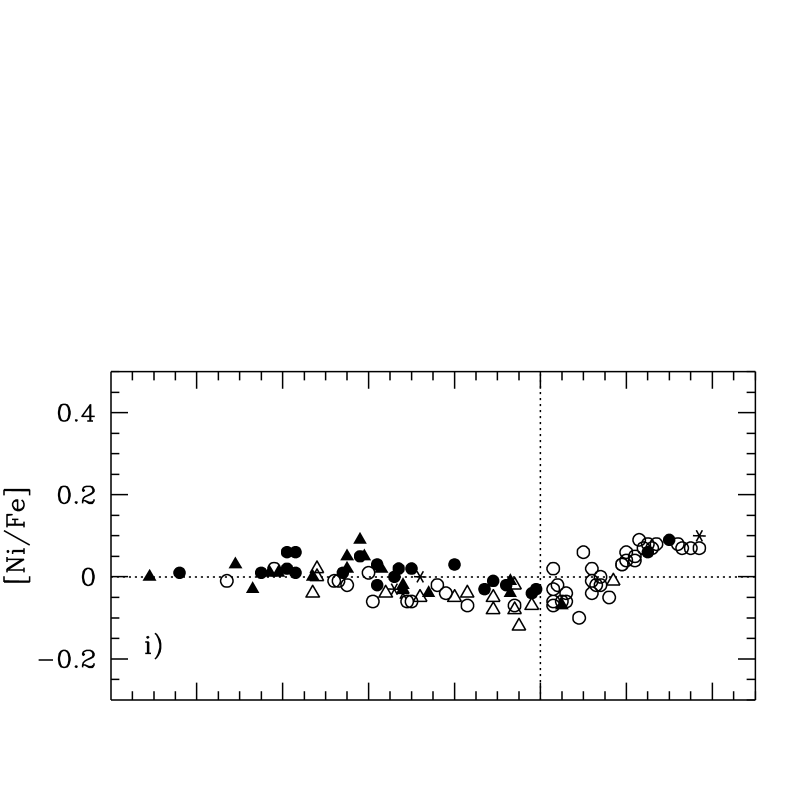
Figure 8: Elemental abundances relative to Fe. Dotted lines indicate solar values. Thin disk and thick disk stars are marked by empty and filled circles, respectively. Stars from Bensby et al. (bensby (2003), 2004a ) are marked by circles and stars from the new northern sample by triangles. Transition objects are marked by asterisks.

O, Mg, Si, Ca, and Ti:

Thin and thick disk stars are clearly separated and show tight and distinct trends. The down-turns (or “knees”) in the [O/Fe] and [Mg/Fe] trends for the thick disk stars are especially prominent (see Fig. 8a and c). There is no doubt that the locations of these “down-turns” are at $\rm[Fe/H]\approx-0.4$ after which [O/Fe] and [Mg/Fe] decline toward solar values. At lower [Fe/H] the trends are essentially flat showing constant values of [Mg/Fe] $\sim+0.35$ and [O/Fe] $\sim+0.4$.

Although not as prominent as for O and Mg, these features are also clearly present for the other three $\alpha$-elements; Si, Ca, and Ti.

Na and Al:

The appearance of the thin and thick disk [Na/Fe] trends (Fig. 8b) show an inverted behaviour compared to the $\alpha$-elements. Instead, the stars in thin disk seem to be more abundant in Na than those in the thick disk. At first glance this [Na/Fe] trend appear to be different from that in Bensby et al. (bensby (2003)) where we found that [Na/Fe] trends for the thin and thick disk appear to be merged. The tighter [Na/Fe] trends in this study (more stars are now used to trace the trends) indicate that also the Na abundances are distinct between the two disk populations, even if not as well separated as for the $\alpha$-elements.

The Al trends show the same type of trends as the $\alpha$-elements (see Fig. 8d). This supports our findings in Bensby et al. (bensby (2003)) that Al and the $\alpha$-elements are produced in the same environments and have been dispersed into the interstellar medium on the same time-scales, i.e., the SN II events. Also, McWilliam (mcwilliam (1997)) noted that Al, from a phenomological point of view, can be classified as an $\alpha$-element.

Cr and Ni:

Cr varies tightly in lock-step with Fe (see Fig. 8h). No trends are seen and the thin and thick disk stars are well mixed which strongly emphasize the common origin for Cr and Fe.

In Bensby et al. (bensby (2003)) we found that the Ni and Fe below solar metallicities evolve roughly in lockstep (i.e., [Ni/Fe] $\approx$ 0). At [Fe/H] $\sim$ 0 the [Ni/Fe] trend then showed a prominent up-turn that had not been seen in previous studies. This deviation from a flat [Ni/Fe] trend has an impact on the oxygen abundances that are derived from the forbidden [O i] line at 6300 Å since this line is heavily blended by two Ni i lines (see Bensby et al. 2004a ). In the new sample there are only two stars with [Fe/H] $>0$. They do, however, follow the same trend as found in Bensby et al. (bensby (2003)) and show an increased [Ni/Fe] (see Fig. 8i). The now larger number of stars at [Fe/H] $<0$ also indicates that it is possible that the [Ni/Fe] trend at these metallicities actually is not flat. We see a slight overall decrease in [Ni/Fe] when going to higher [Fe/H], and at [Fe/H] $=0$ there is an underabundance of Ni relative Fe of about 0.05 dex. There is also a weak tendency that the thick disk stars are more abundant in Ni than the thin disk stars.

Zn:

The [Zn/Fe] trend is tight and in accordance with Bensby et al. (bensby (2003)) (see Fig. 8j). This is somewhat surprising since the trend for the new stars is based on one Zn i line only. Further, this is also the line that we rejected from further analysis in Bensby et al. (bensby (2003)) since it was suspected to have a hidden blend that was growing with metallicity. For metallicities below [Fe/H] $\approx 0$ we, however, found that the blend should have less influence. This is most likely the reason for the good agreement between our [Zn/Fe] trends.

Comparing our thin disk [Zn/Fe] trend with Reddy et al. (reddy (2003)) we see that in the range $\rm-0.4\lesssim[Fe/H]\lesssim-0.2$ their stars have [Zn/Fe] in the range $-0.1$ dex to $+0.2$ dex. This is higher than what we see for our thin disk stars that have [Zn/Fe] in the range $-0.1$ dex to $0$ dex in the same metallicity bin. Our thick disk stars have [Zn/Fe] in the range $0$ dex to $+0.2$ dex which means that by combining the [Zn/Fe] trends for our thin and thick disks we would see the same spread in [Zn/Fe] as Reddy et al. (reddy (2003)). However, as we saw in Sect. 5.3, there seem to be an offset of about $0.05--0.10$ dex between our [Zn/Fe] abundances and those in Reddy et al. (reddy (2003)). Taking this into account will put our thin disk [Zn/Fe] trend on the same level as the one in Reddy et al. (reddy (2003)), or vice versa. But, it will not give any insight into why the thin disk [Zn/Fe] trend in Reddy et al. (reddy (2003)) show a larger scatter than what we see in our [Zn/Fe] trend. It is probably due to the analysis in which only one or two spectral lines are analyzed, which unevitably leads to larger internal errors unless extreme care is taken.

7.2 [$\alpha$/Fe] at different Z_max

Figure 9: [O/Fe] versus $Z_{\rm max}$ for the 36 stars from this study and the 66 stars from Bensby et al. (bensby (2003)). Thin disk and thick disk stars are marked by empty and filled circles, respectively. Transition objects are marked by asterisks.

Figure 10: Abundance trends in the thick disk for oxygen. The thick disk sample has been divided into two sub-groups: stars that have $Z_{\rm max}>500$ pc (open squares); and stars that have $Z_{\rm max}\leq 500$ pc (open stars).

Since our thick disk stellar sample is far from complete and is biased towards higher metallicities we can not use it to probe for vertical gradients in the thick disk metallicity distribution. However, it can be used to investigate if there are differences in the abundance trends at various heights above the Galactic plane. If the trends are similar this would indicate that the thick disk stars come from a stellar population that initially was homogeneous and well mixed.

The maximum vertical distance ($Z_{\rm max}$) a star can reach above the plane can be estimated from (L. Lindegren 2003, priv. comm.):

$$Z_{\rm max}=\sqrt{Z^{2}+(k\cdot W_{\rm LSR})^{2}},$$ (1)

where

$$k\,=\,(85\,{\rm Myr})\,/\,(2\,\cdot\,\pi)\,({\rm pc\,/\,Myr})\,/\,({\rm km\,/\,s}),$$ (2)

and $Z$ is the present distance of the star from the Galactic plane (in pc) and $W_{\rm LSR}$ is its present velocity in the $Z$-direction. Equation (1) assumes that stars in the solar neighbourhood oscillates harmonically in the $Z$-direction with a period of 85 Myr, independent of their other motions. Since the density of stars decreases with $|Z|$, Eq. (1) will underestimate $Z_{\rm max}$ for stars that have large $W_{\rm LSR}$ velocities. The relationship is however sufficient for our purposes.

Figure 11: Elemental abundances relative to Fe. Dotted lines indicate solar values. Thin disk and thick disk stars are marked by empty and filled circles, respectively. Transition objects are marked by asterisks.

Figure 9 shows the [O/Fe] ratio as a function of $Z_{\rm max}$ for our sample. The thin disk stars are all confined to within $\sim$ 300 pc of the Galactic plane, whereas the thick disk stars move in orbits reaching vertical distances up to 1 kpc or more. Dividing the thick disk sample at $\sim$ 500 pc give two sub-samples of approximately equal sizes.

As can be seen in Fig. 10 the [O/Fe] trends for the two sub-samples are the same. An important point is that the ”knee” is located at the same [Fe/H] for both sub-samples. If the Galactic thick disk formed in a fast dissipational collapse, with a proposed time scale of $\sim$ 400 Myr (see, e.g., Burkert et al. burkert (1992)), it is likely that the position of the ”knee” would differ in the two sub-samples. SN II that have a time-scale of typically 10 Myr would then have time to enrich the interstellar medium with even more of the $\alpha$-elements at higher [Fe/H] in the thick disk sub-sample that formed closer to the Galactic plane. The invariance of our abundance trends with distance from the plane instead indicates that the thick disk stellar population was well mixed before it got kinematically heated. This can for example be accomplished if the stars in a pre-existing old thin disk got kinematically heated by the tidal interaction with a companion galaxy that either merged with, or passed close by, the Galaxy.

7.3 The $r$- and $s$-process element abundance trends

Figure 11a–c shows our results for the $r$- and $s$-process elements Y, Ba, and Eu with Fe as the reference element, and Fig. 11d–f with oxygen as the reference element.

Eu:

Eu is supposed to be an almost pure $r$-process element (approximately 94 % $r$-process and 6 % $s$-process, Arlandini et al. arlandini (1999)) which means that it mainly should come from SN II where the neutron flux is sufficient for the $r$-process to occur (i.e. the neutron density is so high that the neutron-capture timescale is much smaller than the $\beta$-decay timescale). The [Eu/Fe] trend in Fig. 11a is very similar to the [O/Fe] trend in Fig. 8a. The thick disk [Eu/Fe] trend also shows a turn-over at [Fe/H] $\approx-0.4$, and the thin disk [Eu/Fe] trend shows the same shallow decline over the whole range in [Fe/H]. The downward trend that we found for [O/Fe] at [Fe/H] $>0$ is also present in [Eu/Fe] but with a larger scatter. The generally good agreement between Eu and oxygen, which is further illustrated in Fig. 11f where we plot [Eu/O] versus [O/H], indicates that these two elements indeed originate from the same type of environments.

Our [Eu/Fe] trend for the thin disk is in good agreement with previous studies (Woolf et al. woolf (1995); Koch & Edvardsson koch (2002); Mashonkina & Gehren mashonkina (2001)), and our thick disk [Eu/Fe] trend is in agreement with Mashonkina & Gehren (mashonkina (2001)) for the metallicities where their thick disk stars overlap with ours (i.e. [Fe/H] $\lesssim-0.3$). The continuing decline that we see in [Eu/Fe] for the thick disk for [Fe/H] $>-0.3$ is, on the other hand, new.

Ba and Y:

The s-process contributions to the solar composition is for Ba 81 % (Arlandini et al. arlandini (1999), but see also Travaglio et al. travaglio (1999)) and for Y 74% (Travaglio et al. travaglio2 (2004)). In the $s$-process the neutron flux is low, which means that the radioactive isotopes will have time to $\beta$-decay between the neutron-captures. Probable sites for the $s$-process are the atmospheres of stars on the asymptotic giant branch (AGB stars) (e.g., Busso et al. busso (1999)). If this is the case the enrichment of the $s$-process elements to the interstellar medium probably occur on a timescale similar to elements originating in SN Ia.

The [Y/Fe] and [Ba/Fe] trends are different for the thin and thick disks (Fig. 11a and b). Especially [Ba/Fe] is distinct and well separated for the two disks. For the thick disk stars the [Ba/Fe] trend (Fig. 11b) is flat, lying on a solar ratio. [Y/Fe] for the thick disk shows a larger scatter and has a flat appearance with underabundances between 0 and $-0.2$ dex (Fig. 11a). The thin disk [Ba/Fe] trend shows a prominent rise from the lowest [Fe/H] until reaching solar metallicities, after which it starts to decline. The [Y/Fe] trend for the thin disk is similar but shows a considerably larger scatter and not such a well-defined trend as that for [Ba/Fe].

7.4 Evolution of Ba and Eu

Figure 12: An illustration of the relative contributions from the $r$- and $s$-process to the elements Eu and Ba. The dotted line shows the pure $r$-process contribution to Eu and Ba while the full line shows the solar system mix of $r$- and $s$-process contributions (Arlandini et al. arlandini (1999)). Thin and thick disk stars are marked by open and filled circles, respectively. Transition objects are marked by asterisks ($\ast$), and ’open stars’ data from Burris et al. (burris (2000)).

Figure 13: [Eu/Ba] versus [Fe/H]. The dashed lines show the pure r-process ratio which is [Eu/Ba] = 0.7 and has been calculated from the yields given in Arlandini et al. (arlandini (1999)).

In Fig. 12 we compare our Eu and Ba data with predictions for pure $r$-process composition ($\rm[Eu/Ba]=0.7$, calculated from the yields given in Arlandini et al. arlandini (1999)) and a solar mixture of $r$- and $s$-process contributions (i.e., $\rm[Eu/Ba]=0$). Also included in this plot are low-metallicity halo stars (giants) from Burris et al. (burris (2000)). The thin disk shows a solar system mix for all metallicities while the thick disk has not yet experienced the full contribution of $s$-processed material from low mass AGB stars, i.e., it is closer to the pure $r$-process line.

A first tentative interpretation of these results is that star formation went on long enough in the thick disk so that AGB stars started to contribute to the chemical enrichment, but only just long enough that a solar system mix was reached. After the formation of stars stopped in the thick disk the remaining gas settled into a new thinner disk. Most likely, fresh material of lower metallicity was accreted before star formation started in what is today’s thin disk. The relative $r$- and $s$-process contributions will not change by this dilution if the infalling material is pristine, so in this case the first thin disk stars to form will retain the mixture that was at the end of star formation in the thick disk. The absolute abundances of Ba and Eu in the thin disk will, however, be shifted towards lower values. If on the other hand, the infalling material has experienced enrichment of $r$- and/or $s$-process elements the mixture should change. Our data appear to indicate that this has not been the case and hence that the infalling material was most likely primordial.

This is further illustrated in Fig. 13 where we plot [Eu/Ba] versus [Fe/H] for our stellar sample only. The most metal-rich thick disk stars (at $\rm[Fe/H]\approx 0$) and the most metal-poor thin disk stars (at $\rm[Fe/H]\approx-0.7$) have approximately the same [Eu/Ba] ratio. So while pristine material falls into the disk the gas (from which the thin disk stars form) gets more metal-poor, the [Eu/Ba ratio is preserved.

7.5 Nucleosynthesis in low mass AGB stars

An interesting result is found when studying the trend of [Y/Ba] versus [O/H], see Fig. 14. For both the thin and thick disks this trend is first flat but after solar metallicity a gentle upward trend is seen. This could be explained as a metallicity effect in AGB nucleosynthesis (Busso et al. busso2 (2001)). Figure 1 in Busso et al. (busso2 (2001)) shows how the relative production of light (e.g. Y) and heavy (e.g. Ba) $s$-process elements change as a function of metallicity. For metallicities below solar the [Y/Ba] ratio is roughly flat, i.e. Y and Ba are produced in the same ratio in the low mass AGB stars. However, around, or slightly above, solar metallicity this balance changes such that the lighter $s$-process elements are favoured over the heavy $s$-process elements. Hence [Y/Ba] increases.

Figure 14: [Y/Ba] versus [O/H] for the a) thick disk stars and in b) for the thin disk stars (with the four “transition” objects included as well).

7.6 Transition objects

In our stellar sample we have four stars whose kinematical properties lie in between the definitions of the thin and thick disk populations that we have used (see Table 1). Depending on the choice of the normalization of the thick disk density in the solar neighbourhood they will alter their classifications as either thin disk or thick disk stars (see discussion in the Appendix). When looking at their chemical compositions we see that they not only are intermediate in terms of kinematics but also in terms of abundances at a given [Fe/H] (see Figs. 8 and 11). Which stellar population these stars should belong to, or if they form a distinct population by their own, can only be investigated with a larger sample of such stars.

7.7 Deviating stars - outliers

From our abundance plots it is evident that not all stars follow the trends as outlined by the majority of stars in the two disk populations. There are, in particular, three stars (HIP 2235, HIP 15510, and HIP 16788) that seem to show suspiciously high abundances in either or both of Y and Ba (see Figs. 11a, b, d, and e). To enable a direct comparison we list their chemical properties in Table 10 and discuss each of them in turn.
HIP 2235 is a thin disk star and has spectral type F6V (according to the Simbad database) and shows high over-abundances in both Ba and Y that is not recognized in any of the other thin disk stars (or the thick disk stars). This s-enhancement can be due to that s-enriched material has been transferred from from a companion star into the stellar atmosphere. The companion star could have been an AGB star, in which these elements are believed to be synthesized (see, e.g., Abia et al. abia (2002)), that now is invisible since it has evolved into a white dwarf.
HIP 15510 is a G8V thick disk star and show an abnormal enhancement in Y but not in Ba. It is not unlikely that this star not has been subject to the same type of mass-transfer as HIP 2235 maybe has been. It is namely well possible to have s-stars with Y-enhancement and no Ba-enhancement and vice versa (see, e.g., review by Busso et al. busso3 (2004)). However, the Y abundance for HIP 15510 is based on one spectral line only, making it highly uncertain.
HIP 16788 is a G0 thick disk star that has no luminosity classification in the Simbad database. However, from our derived $\log g=4.24$ it is most likely also a main sequence star. It is highly enhanced in both Y and Ba as in the case for HIP 2235.

Stars from the “old sample” that show deviating $\alpha$-abundances were discussed in Sect. 9.4 in Bensby et al. (bensby (2003)) to which the reader is referred since none of the new stars showed deviating abundances for these elements.

Table 10: Abundances for deviating stars. Each star has three columns; abundance; line-to-line scatter (1$\sigma$ standard deviation); and (in parenthesis) number of lines that were used to derive the abundance.

	HIP 2235		HIP 15510		HIP 16788
	Thin disk		Thick disk		Thick disk
$\rm[Fe/H]$	$-0.28$	0.07 (65)	$-0.41$	0.08 (69)	$-0.32$	0.07 (78)
$\rm[O/H]$			$-0.01$	0.00 (1)	$-0.27$	0.00 (1)
$\rm[Eu/H]$	$-0.19$	0.00 (1)			$-0.06$	0.00 (1)
$\rm[Ba/H]$	0.54	0.06 (4)	$-0.56$	0.08 (3)	0.63	0.06 (4)
$\rm[Y/H]$	0.31	0.14 (3)	0.09	0.00 (1)	0.45	0.12 (4)

8 Discussion and summary

In this study we have presented a differential abundance analysis between the Galactic thin and thick disks for 14 elements (O, Na, Mg, Al, Si, Ca, Ti, Cr, Fe, Ni, Zn, Y, Ba, and Eu) for a total of 102 nearby F and G dwarf stars (including the stars from our previous studies Bensby et al. bensby (2003), 2004a ). The results from the 36 stars in the new sample further confirms, strengthens, and extends the results presented in Bensby et al. (bensby (2003), 2004a ). Results that are new in this study are those for the $r$- and $s$-process elements Y, Ba, and Eu, where we find the thin and thick disks abundance trends to be distinct and well defined. We also see indications of a metallicity effect in the AGB nucleosynthesis of Y and Ba, such that Y is favoured over Ba at higher [Fe/H]. Our results for Eu show that Eu abundances follow the oxygen abundances very well. This confirms that Eu is an element that mainly is produced in SN II.

In our studies we have included thick disk stars with [Fe/H] $\gtrsim-0.35$, which no other study have. At these higher metallicities we find that the [$\alpha$/Fe] trends, at [Fe/H] $\approx-0.4$, turns over and decline towards solar values where they merge with the thin disk [$\alpha$/Fe] trends. The observed down-turn (or “knee”) in the thick disk [$\alpha$/Fe] trends at [Fe/H] $\approx-0.4$ can be interpreted as a signature of the contribution from SN Ia to the chemical enrichment of the stellar population under study. Massive stars ($M\gtrsim 10$ $\mathcal{M}_{\sun}$) explode as core-collapse supernovae type II (SN II) and enrich the interstellar medium with $\alpha$-elements and lesser amounts of heavier elements such as the iron peak elements (e.g. Tsujimoto et al. tsujimoto (1995); Woosley & Weaver woosley (1995)). Due to the short lifetimes of these massive stars they enrich the interstellar medium in the early phases of the chemical evolution and produce high [$\alpha$/Fe] ratios at the lower metallicities. SN Ia disperse large amounts of iron-peak elements into the interstellar medium and none or little of $\alpha$-elements. Since their low-mass progenitors are expected to have much longer lifetimes than the SN II progenitors (e.g. Livio livio (2001)) there will be a delay in the production of Fe as compared to the $\alpha$-elements. Hence, when SN Ia start to contribute to the enrichment, the [$\alpha$/Fe] ratios will decrease.

The fact that we see the signatures from SN Ia in the thick disk thus means that star formation must have continued in the thick disk for a time that was at least as long as the time-scale for SN Ia. The time-scale for a single SN Ia is very uncertain (see e.g. Livio livio (2001)). However, we have seen from a study of ages and metallicities in the thick disk that it has taken about 2–3 billion years for the thick disk stellar population to reach a metallicity of [Fe/H] $=-0.4$ (Bensby et al. 2004b ). Thus we can tentatively conclude that the SN Ia rate peaked at $\sim 2$–3 billion years from the start of the star formation in the population that we today associate with the thick disk. The age-metallicity relation in the thick disk that we find in that study also indicates that star formation might have continued for 2–3 billion years after the peak in the SN Ia rate in order to reach roughly solar metallicities. The most important conclusion from this is that the thick disk most probably formed during an epoch spanning several ($>2$–3) billion years. Data from solar neighbourhood stars have also shown the SN Ia time-scale to be as long as $\sim$ 1.5 Gyr (Yoshii et al. yoshii (1996)).

We are able to draw further conclusions about the origin and chemical evolution of the thick disk. The observational constraints for a formation scenario of the thick disk are:

1. Distinct, smooth, and separated abundance trends between the thin and thick disks.

2. At a given [Fe/H] below solar metallicities the thick disk stars are more enhanced in their $\alpha$-element abundances than the thin disk

3. The thick disk $\alpha$-element trends show signatures of enrichment from SN Ia.

4. The abundance trends are identical for thick disk stars that reach different heights above the Galactic plane ($>500$ pc and $<500$ pc).

5. The thick disk stars have an older mean age than the thin disk stars

6. AGB stars have contributed to the chemical enrichment of the thick disk but not as much as to the enrichment of the thin disk

• A less well established constraint from this study is that there might be a possible age-metallicity relation in the thick disk indicating that star formation might have continued for several billion years.

Taking these constraints into consideration we argue that the currently most probable formation scenario for the thick disk is an ancient merger event between the Milky Way and a companion galaxy. In this event the stellar population of the thin disk that was present at that time got kinematically heated to the velocity distributions and dispersions that we see in today’s thick disk. We note that recent models of hierarchical galaxy formation might be able to succesfully reproduce thick disks in Milky Way like galaxies and the abundance trends might be fully explainable also in these models (Abadi et al. abadi (2003)).

How can we explain the trends observed in the thin disk? The thin disk stars, on average, are younger than the thick disk stars. However, the low-metallicity tail in the metallicity distribution of the thin disk stars overlap with the metallicity distribution of the thick disk stars. A possible scenario would be that once star formation in the thick disk stops, there is a pause in the star formation. During this time in-falling fresh gas accumulates in the Galactic plane, forming a new thin disk. Also, if there is any remaining gas from the thick disk it will settle down onto the new disk. Once enough material is collected, star formation is restarted in the new thin disk. The gas, though, has been diluted by the metal-poor in-falling gas. This means that the first stars to form in the thin disk will have lower metallicities than the last stars that formed in the thick disk.

Appendix A Kinematical criteria for selecting thick disk stars in the solar neighbourhood

When selecting thin and thick disk stars we assume that the Galactic space velocities ($U_{\rm LSR}$, $V_{\rm LSR}$, and $W_{\rm LSR}$) for the thin disk, thick disk, and stellar halo have Gaussian distributions. The space velocities $U_{\rm LSR}$, $V_{\rm LSR}$, and $W_{\rm LSR}$ were calculated using our measured radial velocities and positions, proper motions, and parallaxes from the Hipparcos catalogue (see Eqs. A.1 – A.4 in Bensby et al. bensby (2003)). For each star we then calculate the probabilities that it belong to either the thin disk ($D$), thick disk ($TD$), or the halo ($H$). By also take the fraction of thick disk stars in the solar neighbourhood into account, the final relationship for calculating the individual probabilities are (see also Bensby et al. bensby (2003)):

$$P=X\cdot k\cdot\exp\left(-\frac{U^{2}_{\rm LSR}}{2\,\sigma_{\rm U}^{2}}-\frac{(V_{\rm LSR}-V_{\rm asym})^{2}}{2\,\sigma_{\rm V}^{2}}-\frac{W^{2}_{\rm LSR}}{2\,\sigma_{\rm W}^{2}}\right),$$ (3)

where $P$ is either $D$, $TD$ or $H$; and

$$k=\frac{1}{(2\pi)^{3/2}\,\sigma_{\rm U}\,\sigma_{\rm V}\,\sigma_{\rm W}},$$ (4)

normalizes the expression; $\sigma_{\rm U}$, $\sigma_{\rm V}$, $\sigma_{\rm W}$ are the characteristic velocity dispersions; $V_{\rm asym}$ is the asymmetric drift; and $X$ is the observed fraction of stars in the solar neighbourhood for each population. We calculated for each star the “relative probabilities” $TD/D$ and $TD/H$. Thin disk stars were selected as those with $TD/D<0.1$ (i.e. at least ten times more probable of being a thin disk stars than a thick disk star) and thick disk stars as those with $TD/D>10$ (i.e. at least ten times more probable of being a thick disk stars than a thin disk star). $TD/H>1$ was required for both the thin and thick disk stars.

Figure 15: CMD for the full stellar sample (12 634 stars).

Of the parameters that has the largest influence on the derived probability ratios, the normalization factor is the one that is the least well constrained. In Bensby et al. (bensby (2003)) we used a value of 6 %. The lowest value 2 % was found by Gilmore & Reid (gilmore (1983)) and Chen (chen2 (1997)). Intermediate values $\sim$ 6 % were found by Robin et al. (robin (1996)) and Buser et al. (buser (1999)), and higher values $\sim$ 15 % by Chen et al. (chen3 (2001)) and Soubiran et al. (soubiran (2003)).

We will here show that an increase of the local normalization of the thick disk stars from 6 % to 10 % (and consequently a lowering of the thin disk density from 94 % to 90 %) is motivated. Changing to 10 % will not influence the thick disk sample in Bensby et al. (bensby (2003)) since the only effect is to raise the $TD/D$ ratios by a factor of $\sim$ 1.7 (see column 2 in Table 12). Instead those thick disk stars will have their classicications strengthened. The thin disk sample in Bensby et al. (bensby (2003)) will not change either since all those stars had their $TD/D$ ratios well below 0.1 (typically 0.01).

We select our stars from the same data set as in Feltzing et al. (feltzing (2001)) and Feltzing & Holmberg (feltzing2 (2000)). In brief this includes all stars in the Hipparcos catalogue (ESA esa (1997)) that have relative errors in their parallaxes less than 25 % and that have published radial velocities (see e.g. Bensby et al. bensby (2003); Feltzing & Holmberg feltzing2 (2000)). This sample consists of 12 634 stars. Note that known binaries have been excluded from the data (see Feltzing et al. feltzing (2001)).

Table 11: Characteristic velocity dispersions ($\sigma_{\rm U}$, $\sigma_{\rm V}$, and $\sigma_{\rm W}$) in the thin disk, thick disk, and stellar halo, used in Eq. (3). $V_{\rm asym}$ is the asymmetric drift.

	$\sigma_{\rm U}$	$\sigma_{\rm V}$	$\sigma_{\rm W}$	$V_{\rm asym}$
	———-  [km s-1]  ———-
Thin disk ($D$)	$\leavevmode\nobreak\ \leavevmode\nobreak\ 35$	20	16	$-15$
Thick disk ($TD$)	$\leavevmode\nobreak\ \leavevmode\nobreak\ 67$	38	35	$-46$
Halo ($H$)	$160$	90	90	$-220$

Table 12: The number of stars in given $TD/D$ intervals for different values on the local density of thick disk stars ($X_{\rm TD}$). The second column indicates the factor by which the $TD/D$ ratios change when varying the normalization (with the 10 % density as base). The corresponding CM-diagrams can be seen in Fig. 16.

$X_{\rm TD}$		—————  $N_{\rm stars}$  —————
		$<$ 0.1	0.1 – 1	1 – 10	$>$ 10
2%	0.2	11781	362	166	261
6%	0.6	11305	689	238	347
10%	1	10969	946	285	383
14%	1.5	10623	1215	327	421

Figure 16: CMDs for different interval of $TD/D$ when changing the local density of thick disk stars (2 %, 6 %, 10 %, and 14 %). The number of stars in each CMD is given in Table 12.

The colour-magnitude diagram (CMD) for all 12 634 stars is shown in Fig. 15. Figure 16 show the CMD for three different $TD/D$ intervals: $0.1<TD/D<1$ (i.e “low probability” thin disk stars); $1<TD/D<10$ (i.e “low probability” thick disk stars); and $TD/D>10$ (i.e “high probability” thick disk stars), with four different values of the thick disk normalization in the solar neighbourhood (2 %, 6 %, 10 %, 14 %). The CMD’s for the “high probability” thin disk (i.e. $TD/D<0.1$). They are all essentially all like the CMD in Fig. 15.

Thick disk ($TD/D>10$):

The first thing that is evident from Fig. 16 is that the proposed thick disk population have a prominent turn-off and that the CMD essentially do not change when going from the lowest to the highest value for the normalization. All stars that move into this $TD/D$ range when raising the normalization come from the $1<TD/D<10$ bin. Hence they are always classified as thick disk stars regardless of the normalization. The prominent turn-off that is seen is typical for an old stellar population which is in concordance with the current beliefs of the Galactic thick disk (see e.g. Fuhrmann fuhrmann (1998)).

Thick disk ($1<TD/D<10$):

The CMD’s for these stars resemble those for the stars with $TD/D>10$. The number of stars in this $TD/D$ range almost double when going to the highest thick disk normalization. As in the case for the $TD/D>10$ stars not much happens at first glance when raising the thick disk normalization. However, when going from the 10 % to the 14 % normalization a few stars with $M_{\rm V}$ $<$ 5 and $B-V$ $<$ 0.5 (i.e. in the upper left area of the CMD) populate the CMD for the higher normalization. These stars are most likely younger objects that should be attributed to the thin disk. A 14 % normalization is therefore possibly too high given the velocity dispersions and rotational lags that we use (see Table 11).

Thin disk ($0.1<TD/D<1$):

A young population such as the thin disk should include young stars, especially the more massive stars that are still located on the main sequence. For the 2 % normalization the CMD look suspiciously like the CMDs for the samples with higher $TD/D$ ratios (i.e. the thick disk stars). The upper left hand area is poorly populated and the CMD probably mainly consists of stars with “hot” thick disk kinematics that have a too low $TD/D$ ratio due to a too low normalization. The picture is improved for the 6 % normalization where a substantial number of young objects start to populate the CMD.

From this simple investigation we conclude that it is likely that a normalization of 2 % is too low and a 14 % normalization probably is too high for the thick disk in the solar neighbourhood. Somewhere in between there is a dividing line where obviously young objects starts to populate the thick disk CMD. The exact value for this normalization is of course also dependent on the assumed velocity dispersions in the disks. With our aaumptions it is however probably located closer to 10 %. We have therefore used $X_{\rm TD}$ $=$ 10 % in the calculation of our probabilities.

Selecting stars for abundance analysis:

Where to put the limit where to assign a star as a “true” thick disk star is however difficult. The most safe way is to make it independent of the thick disk normalization. When doing this we will disregard the 2 % normalization since it is obviously too low, and only consider values on $X_{\rm TD}$ between 6 and 14 %. When calculating the $TD/D$ ratios with the 10 % normalization, stars with $TD/D\gtrsim 2$ will then always have (independent on the value on $X_{\rm TD}$) $TD/D>1$ and can be regarded as thick disk stars. Stars with $TD/D\lesssim 0.6$ will always have (independent on the value on $X_{\rm TD}$) $TD/D<1$ and can be regarded as thin disk stars. Stars having $TD/D$ ratios in between these values will alter their classification as thin or thick disk stars as the normalization increase or decrease (in the range 6 – 14 %). We have therefore referred to these stars as “transition objects” throughout the paper.

References

- (1) Abadi, M.G., Navarro, J.F., Steinmetz, M., & Eke, V.R., 2003, ApJ, 597, 21
- (2) Abia, C., Domínguez, I., Gallino, R., Busso, M., Straniero, O., de Laverny, P., Plez, B., & Isern, J., 2002, ApJ, 579, 817
- (3) Allende Prieto, C., Lambert, D.L., & Asplund, M., 2001, ApJ, 556, L63
- (4) Alonso, A., Arribas, S., & Martínez-Roger, C., 1995, A&A, 297, 197
- (5) Anstee, S.D., & O’Mara, B.J., 1995, MNRAS, 276, 859
- (6) Arlandini, C., Käppeler, F., Wisshak, K., Gallino, R., Lugaro, M., Busso, M., & Straniero, O., 1999, ApJ, 525, 886
- (7) Asplund, M., Gustafsson, B., Kiselman, D., & Eriksson, K., 1997, A&A, 318, 521
- (8) Asplund, M., Grevesse, N., Sauval, A.J., Allende Prieto, C., & Kiselman, D., 2004, A&A, 417, 751
- (9) Barbier-Brossat, M., Petit, M., & Figon, P., 1994, A&AS, 108, 603
- (10) Barklem, P.S., & O’Mara, B.J., 1997, MNRAS, 290, 102
- (11) Barklem, P.S., & O’Mara, B.J., 1998, MNRAS, 300, 863
- (12) Barklem, P.S., O’Mara, B.J., & Ross, J.E., 1998, MNRAS, 296, 1057
- (13) Barklem, P.S., Piskunov, N., & O’Mara, B.J., 2000, A&AS, 142, 467
- (14) Bensby, T., Feltzing, S., & Lundström, I., 2003, A&A, 410, 527
- (15) Bensby, T., Feltzing, S., & Lundström, I., 2004a, A&A, 415, 155
- (16) Bensby, T., Feltzing, S., & Lundström, I., 2004b, A&A, 421, 969
- (17) Burkert, A., Truran, J.W., & Hensler, G., 1992, ApJ, 391, 651
- (18) Burris, D.L., Pilachowski, C.A., Armandroff, T.E., Sneden, C., Cowan, J.J., & Roe, H., 2000, ApJ, 544, 302
- (19) Buser, R., Rong, J., & Karaali, S., 1999, A&A, 348, 98
- (20) Busso, M., Gallino, R., & Wasserburg, G.J., 1999, ARA&A, 37, 239
- (21) Busso, M., Gallino, R., Lambert, D.L., Travaglio, C., & Smith, V.V., 2001, ApJ, 557, 802
- (22) Busso, M., Straniero, O., Gallino, R., & Abia, C., 2004, Carnegie Observatories Astrophysics Series, Vol. 4: Origin and Evolution of the Elements, ed. A. McWilliam and M. Rauch (Cambridge: Cambridge Univ. Press)
- (23) Chen, B., 1997, ApJ, 491, 181
- (24) Chen, Y.Q., Nissen, P.E., Zhao, G., Zhang, H.W., & Benoni, T., 2000, A&AS, 141, 491
- (25) Chen, B., Stoughton, C., Allyn Smyth, J., et al., 2001, ApJ, 553, 184
- (26) Dalcanton, J.J., & Bernstein, R.A., 2002, AJ, 124, 1328
- (27) Edvardsson, B., Andersen, J., Gustafsson, B., Lambert, D.L., Nissen, P.E., & Tomkin, J., 1993, A&A, 275, 101
- (28) ESA, 1997, The Hipparcos and Tycho Catalogues, ESA SP-1200
- (29) Feltzing, S., & Holmberg, J., 2000, A&A, 357, 153
- (30) Feltzing, S., Holmberg, J., & Hurley, J.R., 2001, A&A, 377, 911
- (31) Feltzing, S., Bensby, T., & Lundström, I., 2003, A&A, 397, L1
- (32) Fuhrmann, K., 1998, A&A, 338, 161
- (33) Gallagher, A., 1967, Physical Review, 157, 24
- (34) Gilmore, G., & Reid, N., 1983, MNRAS, 202, 1025
- (35) Gilmore, G., Wyse, R.F.G., & Kuijken, K., 1989, ARA&A, 27, 555
- (36) Gilmore, G., Wyse, R.F.G., & Jones, J.B., 1995, AJ, 109, 1095
- (37) Girardi, L., Bressan, A., Bertelli, G., & Chiosi, C., 2000, A&AS, 141, 371
- (38) Gratton, R.G., Carretta, E., Eriksson, K., & Gustafsson, B., 1999, A&A, 350, 955
- (39) Gratton, R.G., Carretta, E., Matteucci, F., & Sneden, C., 2000, A&A, 358, 671
- (40) Grevesse, N., & Sauval, A.J., 1998, Space Sci. Rev., 85, 161
- (41) Gustafsson, B., Bell, R.A., Eriksson, K., & Nordlund, Å., 1975, A&A, 42, 407
- (42) Ilyin, I.V., 2000, PhD Thesis, University of Oulu
- (43) Johansson, S., Litzén, U., Lundberg, H., & Zhang, Z., 2003, ApJ, 584, L107
- (44) Karlsson, H., & Litzén, U., 1999, Physica Scripta, 60, 321
- (45) Kim, Y.-C., Demarque, P., Yi, S.K., & Alexander, D.R., 2002, ApJS, 143, 499
- (46) Koch, A., & Edvardsson, B., 2002, A&A, 381, 500
- (47) Lawler, J.E., Wickliffe, M.E., Den Hartog, E.A., & Sneden, C., 2001, ApJ, 563, 1075
- (48) Livio, M., 2001, Supernovae and gamma-ray bursts: the greatest explosions since the Big Bang, (eds) M. Livio, N. Panagia, K. Sahu., STScI symp. ser., Vol. 13, p. 334, Cambridge University Press (astro-ph/0005344)
- (49) Mashonkina, L., & Gehren, T., 2000, A&A, 364, 249
- (50) Mashonkina, L., & Gehren, T., 2001, A&A, 376, 232
- (51) Mashonkina, L., Gehren, T., Travaglio, C., & Borkova, T., 2003, A&A 397, 275
- (52) Matteucci, F., 2001, The Chemical Evolution of the Galaxy, Astrophysics and space science library; v. 253, Kluwer Academic Publishers
- (53) McWilliam, A., 1997, ARA&A, 35, 503
- (54) Pitts, R.E., & Newsom, G.H., 1986, J. Quant. Spectrosc. Radiat. Transfer, 35, 383
- (55) Prochaska, J.X., Naumov, S.O., Carney, B.W., McWilliam, A., & Wolfe, A.M., 2000, ApJ, 120, 2513
- (56) Reddy, B.E., Tomkin, J., Lambert, D.L., & Allende Prieto, C., 2003, MNRAS, 340, 304
- (57) Reshetnikov, V., & Combes, F., 1997, A&A, 324, 80
- (58) Robin, A.C., Haywood, M., Créze, M., Ojha, D.K., & Bienaymé, O., 1996, A&A, 305, 125
- (59) Salasnich, B., Girardi, L., Weiss, A., & Chiosi, C., 2000, A&A, 361, 1023
- (60) Schwarzkopf, U., & Dettmar, R.-J., 2000, A&A, 361, 451
- (61) Soubiran, C., Bienaymé, O., & Siebert, A., 2003, A&A, 398, 141
- (62) Sneden, C., McWilliam, A., Preston, G.W., Cowan, J.J., Burris, D.L., & Armosky, B.J., 1996, ApJ, 467, 819
- (63) Tautvaišienė, G., Edvardsson, B., Tuominen, I., & Ilyin, I., 2001, A&A, 380, 579
- (64) Thévenin, F., & Idiart, T. P., 1999, ApJ, 521, 753
- (65) Travaglio, C., Galli, D., Gallino, R., Busso, M., Ferrini, F., & Straniero, O., 1999, ApJ, 521, 691
- (66) Travaglio, C., Gallino, R., Arnone, E., Cowan, J., Jordan, F., & Sneden, C., 2004, ApJ, 601, 864
- (67) Tsujimoto, T., Nomoto, K., Yoshii, Y., Hashimoto, M., Yanagida, S., & Thielemann, F.-K., 1995, MNRAS, 277, 945
- (68) Woolf, V.M., Tomkin, J., & Lambert, D.L., 1995, ApJ, 453, 660
- (69) Woosley, S.E., & Weaver, T.A., 1995, ApJS, 101, 181
- (70) Yi, S., Demarque, P., Kim, Y.-C., Lee, Y.-W., Ree, C.H., Lejeune, T., & Barnes, S., 2001, ApJS, 136, 417
- (71) Yi, S.K., Kim, Y.-C, & Demarque, P., 2003, ApJS, 144, 259
- (72) Yoshii, Y., Tsujimoto, T., & Nomoto, K., 1996, ApJ, 462, 266