Weak lensing in scalar-tensor theories of gravity

Abstract

This article investigates the signatures of various models of dark energy on weak gravitational lensing, including the complementarity of the linear and non-linear regimes. It investigates quintessence models and their extension to scalar-tensor gravity. The various effects induced by this simplest extension of general relativity are discussed. It is shown that, given the constraints in the Solar System, models such as a quadratic nonminimal coupling do not leave any signatures that can be detected while other models, such as a runaway dilaton, which include attraction toward general relativity can let an imprint of about 10%.

I Introduction

The growing evidences for the acceleration of the universe have led to the formulation of numerous scenarios of dark energy (see Ref. peebles03 for reviews). In this construction various routes have been investigated uzan04 . They reduce mainly to the introduction of new degrees of freedom in the cosmological scenario, either as matter fields with negative pressure or in the gravitational sector.

The simplest models accounting for this acceleration rely on the introduction of a slow rolling scalar field whose expectation value varies during the history of the universe. These quintessence models quintessence are characterized by their potential and numerous choices have been discussed in the literature peebles03 . Generically this scalar field may also couple to matter fields wette03 . As a consequence, the values of the fundamental constants will depend on the value of this field and may vary urmp and it will induce a fifth force that will be long range if the scalar field is light, which is usually the case if it is the source of the acceleration of the universe.

In the simplest extension of the quintessence models, the quintessence field universally couples to the other fields. It was realized that the properties of this quintessence field were conserved in that situation uzan99 ; chibamen ; cmb2 . This implies that we are dealing with a scalar-tensor theory of gravity in which the spin-0 partner of the graviton is also the quintessence field. From a phenomenological point of view, extended quintessence models are the simplest well defined theories in which there is a modification of gravity. Various observational signatures on the background evolution, the cosmic microwave background (CMB) anisotropies ru02 ; cmb1 ; cmb2 ; cmb3 ; cmb4 , the big-bang nucleosynthesis have been worked out bp and the reconstruction problem was discussed in details gilles01 . In particular, it was shown that the attraction mechanism toward general relativity dn1 still hold dp in these extended quintessence models, a crucial point since they have to satisfy sharp constraints in the Solar System will . It was also pointed out that a runaway dilaton runaway1 ; runaway2 that does not couple universally, is an appealing models with specific signature such as a variation of some fundamental constants and a violation of the universality of free fall.

Scalar-tensor theories are the most natural alternative to general relativity will ; def , preserving the universality of free fall and constancy of all non gravitational constants. Gravity is mediated not only by a massless spin-2 graviton, corresponding to the spacetime metric, but also by a spin-0 scalar field. Many theoretical motivations to consider such a scalar partner to the graviton have been put forward, particularly in higher-dimensional theories. In string theory, the supermultiplet of the graviton contains a dilaton and moduli fields polchinski .

Scalar-tensor theories are well constrained in the Solar system and one can try to extend these constraints to astrophysical and cosmological scales. In the case of extended quintessence, the effect of the scalar field is important particularly in the recent universe when it starts to dominate. It was pointed out berben that the modification of the equation of state in the recent universe has striking effects on the growth of density perturbation and on weak lensing observables such as the convergence power spectrum.

Weak gravitational lensing has now proven to be a powerful tool to study large scale structures schneider92 ; mellier ; bartelmann01 and to gather information on the nature of the dark energy ludoben ; simpsonbridle . In particular, cross-correlation techniques seem a very promising way to achieve this task (see e.g. cc ). Weak lensing can be detected by the deformation of the shape of background galaxies. It was recently observed by various groups wldetect and can probe the large scale structures of the universe both in the linear and non-linear regimes. Recently, the weak lensing has been studied in the context of generalized cosmologies acqua04 , specializing to quadratic non-minimally coupled models and focusing on the effects on the CMB anisotropies, hence just looking after the linear regime of structure formation. However, as was shown on various examples berben ; ludoben ; tereno04 , the most stringent constraints on cosmological models, able to distinguish dark energy models, arise from the comparison of the linear and non-linear regimes.

In this article, our main goal is to study in details the lensing observable, focusing on 2-point functions to start with, in the case of general relativity and scalar-tensor theories of gravity. In particular, most of the previous studies (e.g. Refs. berben ; ludoben ; tereno04 ) treats the matter power spectrum independently of the CMB anisotropies. We choose to normalize all our spectra on the CMB at low multipole and deduce the lensing observables, both in the linear and non-linear regimes, with the same normalization. Independently of any considerations on the law of gravity, this tool will be of first importance to deal with combined analysis of CMB and lensing data siprop .

Our analysis will be applied to both quintessence and extended quintessence models. We will show that the modification of the equation of state of the universe leaves a detectable imprint on weak lensing observables. Concerning scalar-tensor theories we will show that, given the constraints in the Solar System, many models will let very little signatures. This is the case for instance of a quadratic coupling. Interestingly other models such as a runaway dilaton can have a 10% effect at that is likely to be constrained and/or detected (see Fig. 12). Note that both conclusions are of interest since it will tell us for which class of modifications we have to bother about this extension of the law of gravity.

The article is organized as follows. We first introduce scalar-tensor theories of gravity in § II. In particular, we describe the Einstein and Jordan frames and argue that the latter is the one in which observations take their standard interpretations. We also recall (§ II.2-II.3) the standard constraints on these models and discuss briefly the properties of gravitational lensing (§ II.4). In § III, we derive the distortion of a geodesic light bundle due to large scale structures in a way that is valid for any metric theory of gravity, in particular it does not assume that gravity is described by general relativity and it is valid for scalar-tensor theories. This allows us to define in § IV the weak lensing observables such as the shear power spectrum and the 2-point statistics of the shear field. We then describe our numerical implementation (§ IV.4) in details, as well as the mapping to the non-linear regime. As a first check, we investigate in § V weak lensing in general relativity both for a $\Lambda$CDM and quintessence models. Sec. VI discusses the various effects and differences that arise in scalar-tensor theories of gravity and we then investigate in § VII two families of models: a non-minimally coupled scalar field and runaway dilaton-like models that include attraction toward general relativity.

II General results on scalar-tensor theories

In this article, we focus on scalar-tensor theories of gravity described by the action

$$S = \frac{1}{16\pi G_{*}}\int\mathrm{d}^{4}x\sqrt{-g}\left[F(\varphi)R-g^{\mu\nu}\varphi_{,\mu}\varphi_{,\nu}-2U(\varphi)\right]$$ (1)

$$\qquad\qquad+S_{m}[g_{\mu\nu};\mathrm{matter\;fields}]$$

where $G_{*}$ is the bare gravitational constant from which we define $\kappa_{*}=8\pi G_{*}$. The coupling function $F$ multiplying the Ricci scalar $R$ is dimensionless and needs to be positive to ensure that the graviton carries positive energy. $S_{m}$ is the action of the matter fields that are coupled minimally to the metric, hence ensuring the universality of free fall. The metric has signature $(-,+,+,+)$ and we work in units in which $c=1$.

II.1 Field equations

The variation of action (1) leads to the field equations

$$F(\varphi)G_{\mu\nu} = 8\pi G_{*}T_{\mu\nu}$$ (2)

$$+\partial_{\mu}\varphi\partial_{\nu}\varphi-\frac{1}{2}g_{\mu\nu}\left(\partial_{\alpha}\varphi\right)^{2}-g_{\mu\nu}U(\varphi)$$

$$+\nabla_{\mu}\partial_{\nu}F(\varphi)-g_{\mu\nu}\Box F(\varphi)$$

$$\Box\varphi = U_{,\varphi}-\frac{1}{2}F_{,\varphi}R$$ (3)

$$\nabla_{\mu}T^{\mu\nu} = 0.$$ (4)

Here $\nabla_{\mu}$ is the covariant derivative associated to $g_{\mu\nu}$ and the subscript “${,\varphi}$” denotes the functional derivative with respect to $\varphi$. The stress-energy tensor is defined as

$$T^{\mu\nu}\equiv\frac{2}{\sqrt{-g}}\frac{\delta S_{m}}{\delta g_{\mu\nu}}.$$

Action (1) has been written in the so-called Jordan frame in which matter is universally coupled to the metric. The Jordan metric defines the length and time as measured by laboratory apparatus. In the following, we will be interested in particular in the shape of background galaxies and all observations will have their standard interpretation in this frame def .

It is however useful to define an Einstein frame action through a conformal transformation of the metric

$$g_{\mu\nu}^{*}=F(\varphi)g_{\mu\nu}.$$ (5)

In the following all quantities labelled by a star (*) will refer to Einstein frame. Defining the field $\varphi_{*}$ and the two functions $A(\varphi_{*})$ and $V(\varphi_{*})$ (see e.g. gilles01 ) by

$$\left(\frac{\mathrm{d}\varphi_{*}}{\mathrm{d}\varphi}\right)^{2} = \frac{3}{4}\left(\frac{\mathrm{d}\ln F(\varphi)}{\mathrm{d}\varphi}\right)^{2}+\frac{1}{2F(\varphi)}$$ (6)

$$A(\varphi_{*}) = F^{-1/2}(\varphi)$$ (7)

$$2V(\varphi_{*}) = U(\varphi)F^{-2}(\varphi),$$ (8)

the action (1) reads as

$$S = \frac{1}{16\pi G_{*}}\int\mathrm{d}^{4}x\sqrt{-g_{*}}\left[R_{*}-2g_{*}^{\mu\nu}\partial_{\mu}\varphi_{*}\partial_{\nu}\varphi_{*}-4V(\varphi_{*})\right]$$ (9)

$$\qquad+S_{m}[A^{2}(\varphi_{*})g^{*}_{\mu\nu};\psi].$$

The kinetic terms have been diagonalized so that the spin-2 and spin-0 degrees of freedom of the theory are perturbations of $g^{*}_{\mu\nu}$ and $\varphi_{*}$ respectively. In this frame, the field equations take the form

$$G^{*}_{\mu\nu} = 8\pi G_{*}T^{*}_{\mu\nu}$$ (10)

$$+ 2\partial_{\mu}\varphi_{*}\partial_{\nu}\varphi_{*}-g^{*}_{\mu\nu}\left(\partial_{\alpha}\varphi_{*}\right)^{2}-2g^{*}_{\mu\nu}V$$

$$\Box_{*}\varphi_{*} = V_{,\varphi_{*}}-4\pi G_{*}\alpha(\varphi_{*})T^{*}_{\mu\nu}g_{*}^{\mu\nu}$$ (11)

$$\nabla_{\mu}T^{\mu\nu}_{*} = \alpha(\varphi_{*})T^{*}_{\sigma\rho}g_{*}^{\sigma\rho}\partial_{\nu}\varphi_{*}$$ (12)

where we have defined the Einstein frame stress-energy tensor

$$T^{\mu\nu}_{*}\equiv\frac{2}{\sqrt{-g_{*}}}\frac{\delta S_{m}}{\delta g^{*}_{\mu\nu}},$$

related to the Jordan frame stress-energy tensor by $T_{\mu\nu}^{*}=A^{2}T_{\mu\nu}$. The function

$$\alpha(\varphi_{*})\equiv\frac{\mathrm{d}\ln A}{\mathrm{d}\varphi_{*}}.$$ (13)

characterizes the coupling of the scalar field to matter (we recover general relativity with a scalar field when it vanishes). For completeness, we also define

$$\beta(\varphi_{*})\equiv\frac{\mathrm{d}\alpha}{\mathrm{d}\varphi_{*}}.$$ (14)

Note that in Einstein frame the Einstein equations (10) are the same as the ones obtained in general relativity with a minimally coupled scalar field. Table 1 summarize the notations used in Jordan and Einstein frames.

From these definitions, we can define an effective gravitational constant as

$$G_{\rm eff}=\frac{G_{*}}{F(\varphi)}=G_{*}A^{2}(\varphi_{*})$$ (15)

but, as we shall see, this does not correspond to the Newton constant that will be effectively measured in a Cavendish-like experiment.

Table 1: Notations in Jordan and Einstein frames.

	Jordan frame	Einstein frame
coordinates	$(x,t$)	$(x_{*},t_{*})$
metric	$g_{\mu\nu}$	$g_{\mu\nu}^{*}$
scalar field	$\varphi$	$\varphi_{*}$
potential	$U$	$V$
coupling	$F$	$A$

II.2 Local constraints

Deviations of the theory of gravity from general relativity are sharply constrained in the Solar System will as well as by binary pulsars gilles03 . The constraints are usually set on the post-Newtonian parameters will . In the particular case of scalar-tensor theories, they reduce gilles01 ; def to

$$\gamma^{\mathrm{PPN}}-1 = \frac{F_{,\varphi}^{2}}{F+2F_{,\varphi}^{2}}$$ (16)

$$= -2\frac{\alpha^{2}}{1+\alpha^{2}}$$ (17)

$$\beta^{\mathrm{PPN}}-1 = \frac{1}{2}\frac{\alpha^{2}}{(1+\alpha^{2})^{2}}\frac{\mathrm{d}\alpha}{\mathrm{d}\varphi_{*}}$$ (18)

$$= \frac{1}{4}\frac{FF_{,\varphi}}{2F+3F_{,\varphi}^{2}}\frac{\mathrm{d}\gamma^{\mathrm{PPN}}}{\mathrm{d}\varphi}.$$ (19)

Solar System experiments set sharp constraints on the values of the PPN parameters $(\gamma^{\mathrm{PPN}}_{0},\beta^{\mathrm{PPN}}_{0})$ today. The observed value of the perihelion shift of Mercury implies the bound mercury

$$\left|2\gamma^{\mathrm{PPN}}_{0}-\beta^{\mathrm{PPN}}_{0}-1\right|<3\times 10^{-3}.$$ (20)

The Lunar laser ranging experiment llr imposes

$$4\beta^{\mathrm{PPN}}_{0}-\gamma^{\mathrm{PPN}}_{0}-3=-(0.7\pm 1)\times 10^{-3}$$ (21)

and the measurements of the light deflection by Very Long Baseline Interferometry vlbi improves the constraint on $\gamma^{\mathrm{PPN}}_{0}$ to

$$\left|\gamma^{\mathrm{PPN}}_{0}-1\right|=4\times 10^{-4}.$$ (22)

The recent analysis of the frequency shift of radio waves to and from the Cassini spacecraft have set the even more stringent bound bertotti

$$\gamma^{\mathrm{PPN}}_{0}-1=(2.1\pm 2.3)\times 10^{-5}.$$ (23)

The previous bounds to those obtained in Refs. vlbi ; bertoti were (see Ref. will for a review)

$$\left|\gamma^{\mathrm{PPN}}_{0}-1\right|\leq 2\times 10^{-3},\qquad\left|\beta^{\mathrm{PPN}}_{0}-1\right|\leq 6\times 10^{-4}.$$ (24)

These constraints can be transformed to constraints on the set $(\alpha_{0},\beta_{0})$ (see Ref. gilles03 for a summary). In particular, we can note that binary pulsars imply that $\beta_{0}>-4.5$. The bound (23) implies that

$$\alpha_{0}^{2}\sim\frac{F_{0}^{{}^{\prime}2}}{F_{0}}<4\times 10^{-5}.$$ (25)

The local value of the gravitational constant is deduced from a Cavendish-like experiment, i.e. from the measurement of the Newton force between to masses $m_{1}$ and $m_{2}$, as $G_{\mathrm{cav}}=Fr^{2}/m_{1}m_{2}$. It can be shown def that its theoretical expression is

$$G_{\mathrm{cav}} = \frac{G_{*}}{F}\left(1+\frac{F_{,\varphi}^{2}}{2F+3F_{,\varphi}^{2}}\right)$$ (26)

$$= G_{*}A^{2}(1+\alpha^{2}).$$ (27)

Note that today Eq. (25) implies that $G_{\mathrm{cav}}$ and $G_{\mathrm{eff}}$ do not differ by more than some $10^{-3}$ percent, which is anyhow larger than the accuracy of the measurement of the gravitational constant. At higher redshift this difference may be larger.

Current constraints dickey (see also Ref. urmp for a review) imply that

$$\left|\frac{\dot{G}_{\mathrm{cav}}}{G_{\mathrm{cav}}}\right|_{0}<6\times 10^{-12}\,{\rm yr}^{-1}.$$ (28)

Using Eqs. (13) and (14), this implies that

$$\left|\alpha_{0}+\frac{\beta_{0}\alpha_{0}}{(1+\alpha_{0}^{2})}\right|\left|\dot{\varphi}_{*0}\right|<3\times 10^{-12}\,{\rm yr}^{-1}$$ (29)

All these constraints are local and we will consider in this article only models that satisfy them.

II.3 Cosmological constraints

From a cosmological point of view, there are very few constraints on scalar-tensor theories.

CMB observations may in principle give some constraints but they are often degenerate with other parameters, such as e.g. the cosmological parameters (see e.g. Ref. ru02 ; cmb1 ; cmb2 ; cmb3 ; cmb4 for some studies on the CMB imprints of scalar tensor theories).

More stringent constraints arise from Big Bang nucleosynthesis (BBN). BBN results, and in particular the helium-4 abundance, are very sensitive to the weak interaction freeze-out. This temperature depends on the strength of the gravitational interaction which dictates the expansion rates. BBN mainly requires that (i) the universe is dominated by radiation at the time of nucleosynthesis and (ii) that the number of degrees of freedom of relativistic particles does not vary by more than 20% with respect to its expected value $g_{\rm r}=10.75$. The Friedmann equation (185) for a flat universe reduces to

$${\cal H}^{2}=\kappa_{0}\frac{\pi^{2}}{90}a^{2}g_{\rm r}\left(1+\frac{\delta g_{\rm r}}{g_{\rm r}}\right)T^{4}$$ (30)

with $\delta g_{\rm r}/g_{\rm r}=F_{0}/F(z_{\rm nuc})-1$, if one neglects the contribution of the scalar field to the energy density. Requiring that $\delta g_{\rm r}/g_{\rm r}$ be smaller than 0.2 implies bp that

$$0.8\leq\left|\frac{F_{0}}{F_{\mathrm{nuc}}}\right|=\left|\frac{A^{2}_{\mathrm{nuc}}}{A^{2}_{0}}\right|\leq 1.2.$$ (31)

Let us emphasize that large value of $|{F_{0}}/{F_{\mathrm{nuc}}}|$ were shown to be consistent with the BBN constraints dp if $\beta$ is large enough so that the naive limit (31) can be much more stringent than a detailed study may show.

II.4 A remark on gravitational lensing

Gravitational bending of light by a single mass $M$ in scalar-tensor theory can be derived easily in Einstein frame. Since photons are coupled to the gravitational field only, they are insensitive to the scalar field. One deduces that they are deflected by an angle $\Delta\theta$ exactly in the same way as in general relativity, that is

$$\Delta\theta=4G_{*}A^{2}(\varphi_{*})M/r_{0},$$ (32)

where $A^{2}M$ is the deflecting mass in Einstein frame. $G_{*}$ cannot be measured directly and what we know is only the value of the gravitational constant (26) determined by a Cavendish-like experiment today. Masses attract themselves due to the exchange of both a graviton and a scalar. It follows that

$$G_{\mathrm{cav}}=G_{*}A^{2}_{0}(1+\alpha_{0}^{2})=2\frac{G_{*}A^{2}_{0}}{1+\gamma_{0}}$$ (33)

so that the deflection angle turns out to be

$$\Delta\theta=2(1+\gamma_{0})G_{\mathrm{cav}}M/r_{0}.$$ (34)

In conclusion, the deflected angle is different from the prediction of general relativity, not because photons are deflected differently but because there is a scalar interaction between the test masses which contributes to the value of the effective Newton constant def .

This argument can be straightforwardly generalized to the cosmological context. If the lens seats at a redshift $z$ and if we work in the thin lens approximation then the deflection angle is given by

$$\Delta\theta=4G_{*}A^{2}(z_{\rm lens})M_{\rm lens}/r_{0}.$$ (35)

again, $G_{*}$ cannot be measured and we have access to

$$G_{\mathrm{cav},0}=2\frac{G_{*}A^{2}_{0}}{1+\gamma_{0}}$$ (36)

where the subscript 0 means that it is determined today. It follows that

$$\Delta\theta=2(1+\gamma_{0})G_{\mathrm{cav},0}\frac{M_{\rm lens}}{r_{0}}\frac{A^{2}(z)}{A^{2}(0)}.$$ (37)

The mass of the lensing galaxy, $M_{\rm lens}$, cannot be measured directly.

We mainly expect to have two major effects on lensing observations: (i) an effect of the background dynamics through the angular distances, (ii) a gravitational effect due to the $z$ dependence deflection angle. Eventually, observations of lenses located at different redshift should enable to give an information on $A(z)/A(0)$ as a function of the redshift.

Before we go into a detailed computation, we can give an upper bound on the amplitude of this effect. From the constraint (31), we deduce that the factor depending on $A$ in Eq. (37) has to lie in the range $F_{0}/F(z_{\mathrm{nuc}})\simeq[0.8,1.2]$ so that effects larger than 20% are unlikely to happen, independently of any model (see however Ref. dp ). Let us stress that, as we shall see, the dominant effect will arise from the growth of the density field and not from the two effects we have just mentioned.

To finish this general discussion let us emphasize that we could have added a coupling of the scalar field to the electromagnetic tensor of the form

$$B(\varphi)F_{\mu\nu}F^{\mu\nu}$$ (38)

in the action (1). Such a term will induce a variation of the fine structure constant (see e.g. Ref. urmp for a review), that has to be smaller than $10^{-5}$ between $z\sim 3$ and today, and a violation of the universality of free fall. Interestingly, such a term will not affect the equation of propagation of photons in the eikonal approximation at first order and thus weak lensing observables that are considered in this article.

III Light propagation in a perturbed FLRW spacetime

This section is devoted to the general theory of gravitational lensing. Our construction is based on the geodesic deviation of a bundle of null geodesics and will then be valid as soon as light travels on such null geodesics, which is the case in particular in general relativity and scalar-tensor theories of gravity. § III.1 reviews the standard derivation on the propagation of a light bundle and defines the shear and convergence. In § III.2 and § III.3, we apply this formalism to a Friedmann-Lemaître spacetime and then to a perturbed spacetime in order to get the final expression of the shear.

III.1 General derivation

Let us consider the evolution of a light bundle in a spacetime with metric $g_{\mu\nu}$ following the original work of Ref. sachs62 along the lines of Ref. ub00 . The worldline of each geodesic can be decomposed as

$$x^{\mu}(\lambda)=\bar{x}^{\mu}(\lambda)+\xi^{\mu}(\lambda)$$ (39)

where $\bar{x}^{\mu}(\lambda)$ is a fiducial null geodesic of the bundle and $\lambda$ is an affine parameter along this geodesic. $\xi^{\mu}$ is a displacement vector that labels the other geodesics of the bundle. The tangent vector $k^{\mu}$ along the fiducial geodesic satisfies

$$k_{\mu}k^{\mu}=0,\quad k^{\nu}\nabla_{\nu}k^{\mu}=0.$$ (40)

We assume that the geodesic bundle is converging at the observer’s position $O$. We assume $\lambda$ to vanish in $O$ and to increase toward the past. In $O$ we also choose a quasi-orthonormal reference frame $\{k^{\mu},u^{\mu},n_{1}^{\mu},n_{2}^{\mu}\}$, where $u^{\mu}$ is the 4-velocity of the observer and satisfies

$$u^{\mu}u_{\mu}=-1$$ (41)

and $n_{1}^{\mu},n_{2}^{\mu}$ are two the spacelike vectors spanning the plan orthogonal to the fiducial light ray, i.e. to the line of sight. They satisfy

$$n_{a}^{\mu}n^{b}_{\mu}=\delta_{a}^{b},\quad n_{a}^{\mu}k_{\mu}=n_{a}^{\mu}u_{\mu}=0$$ (42)

with $a,b=1,2$. From this tetrad constructed in $O$, we construct a basis at each point of the geodesic by parallel transporting it along the fiducial geodesic.

As shown in Ref. ub00 , $\xi^{\mu}$ can be decomposed as

$$\xi^{\mu}=\xi_{0}k^{\mu}+\sum_{a=1,2}\xi_{a}n_{a}^{\mu}$$ (43)

and one can always choose to set $\xi_{0}=0$. The propagation equation of $\xi^{\mu}$ is obtained from the geodesic deviation equation as

$$\frac{D^{2}}{\mathrm{d}\lambda^{2}}\xi^{\mu}=R^{\mu}_{\;\;\nu\alpha\beta}k^{\nu}k^{\alpha}\xi^{\beta},$$ (44)

where $R^{\mu}_{\;\;\nu\alpha\beta}$ is the Riemann tensor and ${D}/{\mathrm{d}\lambda}\equiv k^{\mu}\nabla_{\mu}$. In terms of the decomposition (43), this equation reads

$$\frac{\mathrm{d}^{2}}{\mathrm{d}\lambda^{2}}\bm{\xi}=\bm{\mathcal{R}}\bm{\xi},$$ (45)

where $\mathcal{R}^{b}_{\;a}\equiv R^{\mu}_{\;\;\nu\alpha\beta}k^{\nu}k^{\alpha}n_{\mu}^{a}n_{b}^{\beta}$ is known as the optical tidal matrix. We have used the notation $\bm{\xi}=\xi_{a}$ and $\bm{\mathcal{R}}\bm{\xi}=\mathcal{R}^{b}_{\;\;a}\xi_{b}$. Decomposing the Riemann tensor in terms of the Ricci and the Weyl tensor, it can be rewritten as

$$\mathcal{R}^{b}_{\;a}=-\frac{1}{2}R_{\mu\nu}k^{\mu}k^{\nu}\delta^{a}_{b}+C^{\mu}_{\;\;\nu\alpha\beta}k^{\nu}k^{\alpha}n_{\mu}^{a}n_{b}^{\beta}.$$ (46)

The linearity of the geodesic equation implies that $\bm{\xi}$ can be related to the initial value of $\mathrm{d}\bm{\xi}/\mathrm{d}\lambda$ through a linear transformation

$$\bm{\xi}(\lambda)=\bm{\mathcal{D}}(\lambda)\frac{\mathrm{d}\bm{\xi}}{\mathrm{d}\lambda}(0).$$ (47)

Using that $\bm{\xi}(0)=0$ (bundle converging in $O$) , Eq. (45) gives an equation of evolution for $\mathcal{D}^{b}_{a}$ as

$$\frac{\mathrm{d}^{2}}{\mathrm{d}\lambda^{2}}\bm{\mathcal{D}}=\bm{\mathcal{R}}\bm{\mathcal{D}}.$$ (48)

The initial conditions in $0$ for the matrix $\bm{\mathcal{D}}$ are given by

$$\bm{\mathcal{D}}(0)=0\quad\mbox{and}\quad\bm{\mathcal{D}}^{\prime}(0)=\bm{\mathcal{I}},$$ (49)

with $\bm{\mathcal{I}}$ being the $2\times 2$ identity matrix. The matrix $\bm{\mathcal{D}}$ describes the deformation of the light bundle induce by the spacetime geometry.

The direction of observation, $\bm{\theta}_{I}$, and and the angular position of the source $\bm{\theta}_{S}$ are related to the displacement field by

$$\bm{\theta}_{I}=\frac{\mathrm{d}\bm{\xi}}{\mathrm{d}\lambda}(0),\qquad\bm{\theta}_{S}=\frac{\bm{\xi}(\lambda_{S})}{D_{A}(\lambda_{S})}$$ (50)

where $\lambda_{S}$ is the value of the affine parameter at the source and $D_{A}$ is, by definition, the angular distance of the source. It follows that Eq. (47) takes the form

$$\bm{\theta}_{S}=\frac{\bm{\mathcal{D}}(\lambda_{S})}{D_{A}(\lambda_{S})}\bm{\theta}_{I}.$$ (51)

The deformation of the shape of background galaxies is thus characterized by the amplification matrix

$$\bm{\mathcal{A}}\equiv\frac{\mathrm{d}\bm{\theta}_{S}}{\mathrm{d}\bm{\theta}_{I}}=\frac{\bm{\mathcal{D}}(\lambda_{S})}{D_{A}(\lambda_{S})}.$$ (52)

It can always be decomposed as

$$\bm{\mathcal{A}}\equiv\begin{pmatrix}1-\kappa-\gamma_{1}&\gamma_{2}\\ \gamma_{2}&1-\kappa+\gamma_{1}\end{pmatrix},$$ (53)

in terms of the convergence $\kappa$ and of the shear $\bm{\gamma}=(\gamma_{1},\gamma_{2})$. They can be extracted from the amplification matrix as

$$\kappa=1-\frac{1}{2}\,\mathrm{Tr}\,\bm{\mathcal{A}},\qquad\bm{\gamma}=\frac{1}{2}\begin{pmatrix}\mathcal{A}_{22}-\mathcal{A}_{11}\\ 2\mathcal{A}_{12}\end{pmatrix}.$$ (54)

As was emphasized by many authors mellier ; schneider92 ; bartelmann01 and demonstrated experimentally by various observations wldetect , the shear can be obtained from the measurement of the shape of galaxies.

All the definitions and derivations of this section do not depend on the specific form of the metric and are thus completely general as long as photons follow null geodesic and the geodesic deviation equation holds.

III.2 Background spacetime

We now apply this general results to the case of a background cosmological spacetime with line element

$$\mathrm{d}s^{2}=g_{\mu\nu}\mathrm{d}x^{\mu}\mathrm{d}x^{\nu}=a^{2}(\eta)\bar{g}_{\mu\nu}\mathrm{d}x^{\mu}\mathrm{d}x^{\nu}$$ (55)

where $\eta$ is the conformal time and $a$ the scale factor. We decompose the metric as

$$\bar{g}_{\mu\nu}\mathrm{d}x^{\mu}\mathrm{d}x^{\nu}=-\mathrm{d}\eta^{2}+\gamma_{ij}\mathrm{d}x^{i}\mathrm{d}x^{j}$$ (56)

where $\gamma_{ij}$ is the metric of the constant time hypersurfaces. Since they are hypersurfaces of constant curvature

$$\gamma_{ij}\mathrm{d}x^{i}\mathrm{d}x^{j}=\mathrm{d}\chi^{2}+S_{K}^{2}(\chi)\mathrm{d}\Omega^{2}$$ (57)

where $\chi$ is the comoving radial coordinate and $\mathrm{d}\Omega^{2}$ the infinitesimal solid angle. The function $S_{K}$ is defined by

$$S_{K}(\chi)=\frac{\sin(\sqrt{K}\chi)}{\sqrt{K}},\,\chi,\,\frac{\sinh(\sqrt{-K}\chi)}{\sqrt{-K}}$$ (58)

respectively for $K>0,K=0,K<0$.

From Eq. (57), it is clear that $S_{K}$ is the comoving angular distance so that the angular distance will be given by

$$D_{A}=a(\eta)S_{K}(\chi)=a_{0}\frac{S_{K}(\chi)}{1+z}$$ (59)

where $a_{0}$ refers to the value of the scale factor today and $z=a_{0}/a-1$ is the redshift. The expression of $\chi(z)$ is given by

$$\chi(z)=\frac{1}{H_{0}a_{0}}\int_{0}^{z}\frac{\mathrm{d}z}{E(z)}$$ (60)

where $H_{0}$ is the value of the Hubble constant today and $E(z)$ is defined by

$$E(z)=H(z)/H_{0}=(1+z){\cal H}/{\cal H}_{0}.$$ (61)

The expression for $E(z)$ depends on the matter content of the universe and on the theory of gravity. It is given in Appendix B.

To solve Eq. (48), we will use the fact that null geodesics are left unchanged by a conformal transformation since two conformal spaces have the same causal structure (see e.g. Ref. wald ). For the metric $\bar{g}_{\mu\nu}$, Eq. (48) takes the form

$$\frac{\mathrm{d}^{2}}{\mathrm{d}\lambda^{2}}\bm{\mathcal{D}}=-K\bm{\mathcal{D}}.$$ (62)

The solution of this equation is trivially given by

$$\bm{\mathcal{D}}^{(0)}(\lambda)=S_{K}(\lambda)I,$$ (63)

where $S_{K}$ is given by Eq. (58), so that

$$\bm{\mathcal{A}}^{(0)}=\bm{\mathcal{I}}$$ (64)

where the subscript 0 refers to the solutions in the background spacetime.

III.3 Perturbed spacetime

III.3.1 Amplification matrix

Let us now turn to the perturbed cosmological spacetime with a metric

$$ds^{2} = a^{2}(\eta)\left(\bar{g}_{\mu\nu}+h_{\mu\nu}\right)\mathrm{d}x^{\mu}\mathrm{d}x^{\nu}.$$ (65)

Again, we work in the static conformal spacetime with metric $\bar{g}_{\mu\nu}+h_{\mu\nu}$. As usual, we develop the tidal matrix as

$$\bm{\mathcal{D}}=\bm{\mathcal{D}}^{(0)}+\bm{\mathcal{D}}^{(1)}+\mathcal{O}\left(h^{2}\right),$$ (66)

where $\bm{\mathcal{D}}^{(n)}$ involves terms of $n$-th order in the metric perturbation, and consistently we solve Eq. (48) order by order. Plugging the zeroth order solution (64), Eq. (48) reduces to

$$\frac{\mathrm{d}}{\mathrm{d}\lambda}\bm{\mathcal{D}}^{(1)}=\bm{\mathcal{R}}^{(1)}(\lambda)S_{K}(\lambda).$$ (67)

the solution of which is explicitly given by

$$\bm{\mathcal{D}}^{(1)}(\lambda)=\int_{0}^{\lambda}S_{K}(\lambda^{\prime})S_{K}(\lambda-\lambda^{\prime})\bm{\mathcal{R}}^{(1)}(\lambda^{\prime})\mathrm{d}\lambda^{\prime},$$ (68)

so that the amplification matrix is

$$\bm{\mathcal{A}}^{(1)}(\lambda)=\int_{0}^{\lambda}\frac{S_{K}(\lambda^{\prime})S_{K}(\lambda-\lambda^{\prime})}{S_{K}(\lambda)}\bm{\mathcal{R}}^{(1)}(\lambda^{\prime})\mathrm{d}\lambda^{\prime}.$$ (69)

This expression is again very general and just assumes that photons are propagating along null geodesics. Now, we just need to express $\bm{\mathcal{R}}^{(1)}$ in terms of the perturbations of the metric and go back to the original (non static) spacetime to get the final result.

III.3.2 Deflecting potential

To go further, we assume that the perturbations can be decomposed as

$$\frac{1}{2}h_{\mu\nu}\mathrm{d}x^{\mu}\mathrm{d}x^{\nu} = -\phi\mathrm{d}\eta^{2}+B_{i}\mathrm{d}\eta\mathrm{d}x^{i}$$ (70)

$$+\left(-\psi\gamma_{ij}+\bar{E}_{ij}\right)\mathrm{d}x^{i}\mathrm{d}x^{j}$$

where $\phi$ and $\psi$ are the two gravitational potentials in Newtonian gauge, $B_{i}$ and $\bar{E}_{ij}$ describe the vector and tensor perturbations and satisfy

$$\bar{E}_{i}^{i}=D_{i}\bar{E}^{i}_{j}=D_{i}B^{i}=0$$ (71)

where $D_{i}$ is the covariant derivative associated to the spatial metric $\gamma_{ij}$. Using that $2R_{\mu\nu\alpha\beta}=h_{\nu\alpha,\mu\beta}+h_{\mu\beta,\nu\alpha}-h_{\alpha\mu,\nu\beta}-h_{\nu\beta,\alpha\mu}$, we obtain that

$$\mathcal{R}^{(1)}_{ab}=\frac{1}{2}h_{\mu\nu,\alpha\beta}k^{\mu}k^{\nu}n_{a}^{\alpha}n_{b}^{\beta}-\frac{1}{2}\frac{\mathrm{d}}{\mathrm{d}\lambda}\left(\Gamma_{\rho\beta}^{\alpha}\bar{g}_{\alpha\mu}k^{\beta}n_{a}^{\mu}n_{b}^{\rho}\right),$$ (72)

where $\Gamma_{\rho\beta}^{\alpha}$ are the Christoffel symbols. If we focus on scalar perturbations then the second term vanishes and we end up with

$$\mathcal{R}^{(1)}_{ab}=-\partial_{ab}\Phi$$ (73)

where the deflecting potential is defined as

$$\Phi=-\frac{1}{2}h_{\mu\nu}k^{\mu}k^{\nu}.$$ (74)

In the case of a perturbed cosmological spacetime, it reduces to

$$\Phi=\phi+\psi-B_{i}\theta^{i}-\bar{E}_{ij}\theta^{i}\theta^{j}$$ (75)

where $\theta^{i}$ is the direction of observation. This potential includes the effect of rotation and of gravity waves. Notes that in the case of pure scalar perturbation in general relativity and in the absence of anisotropic stress $\phi=\psi$ and we recover the standard result $\Phi=2\phi$.

III.3.3 Final form

The last step requires to go back to the original (non static) metric to get

$$\mathcal{A}_{ab} = I_{ab}$$

$$- \int_{0}^{\chi}\frac{S_{K}(\chi^{\prime})S_{K}(\chi-\chi^{\prime})}{S_{K}(\chi)}\partial_{ab}\Phi\left[S_{K}(\chi^{\prime})\bm{\theta},\chi^{\prime}\right]\mathrm{d}\chi^{\prime}.$$

It follows that the shear is given by by the trace of this matrix

$$\kappa(\bm{\theta},\chi) = \frac{1}{2}\int_{0}^{\chi}\frac{S_{K}(\chi^{\prime})S_{K}(\chi-\chi^{\prime})}{S_{K}(\chi)}\Delta_{2}\Phi\,\mathrm{d}\chi^{\prime},$$ (77)

with $\Delta_{2}\equiv\partial_{a}\partial^{a}$. The deflecting potential is evaluated along the line of sight as $\Phi=\Phi\left[S_{K}(\chi^{\prime})\bm{\theta},\chi^{\prime}\right]$.

In this derivation, the source has been assumed to be at a given redshift, it generalizes easily to a more general redshift distribution, $p_{\chi}(\chi)\mathrm{d}\chi$, as

$$\kappa(\bm{\theta})=\int p_{\chi}(\chi)\kappa(\bm{\theta},\chi)\mathrm{d}\chi.$$ (78)

In conclusion, the shear takes the form

$$\kappa(\bm{\theta}) = \frac{1}{2}\int_{0}^{\chi_{\rm H}}g(\chi)S_{K}(\chi)\Delta_{2}\Phi\left[S_{K}(\chi)\bm{\theta},\chi\right]\mathrm{d}\chi.$$ (79)

where $g$ is defined as

$$g(\chi) = \int_{\chi}^{\chi_{\rm H}}p(\chi^{\prime})\frac{S_{K}(\chi^{\prime}-\chi)}{S_{K}(\chi^{\prime})}.$$ (80)

III.4 Comments

Again, let us stress that this construction does not assume the validity of general relativity. It is based only on the validity of the geodesic deviation equation. This is the case in particular for all metric theory of gravity such as scalar-tensor theories.

We also emphasize that using a conformal transformation to solve the problem in a static spacetime has greatly simplified the derivation.

In the late universe, when we are interested by gravitational lensing effects, the matter content is mainly dominated by pressureless matter and dark energy. It follows that we can define an effective density field, $\delta_{\mathrm{eff}}$, by the relation

$$\Delta{\Phi}={3}H_{0}^{2}\Omega_{m,0}\frac{\delta_{\mathrm{eff}}}{(a/a_{0})}$$ (81)

where $\Omega_{m,0}$ is the value of the matter density parameter today. The subsecript “$m$” refers to the matter fields, including at least two components, dark matter (cdm) and baryonic matter (b). If we express the 3-dimensional Laplacian as $\Delta_{2}+\partial^{2}_{z}$ where $\partial_{z}$ is the derivative along the line of sight, then the convergence (79) can be expressed in terms of the effective density contrast as

$$\kappa(\bm{\theta})=\frac{3}{2}H_{0}^{2}\Omega_{m,0}\int_{0}^{\chi_{\rm H}}g(\chi)S_{K}(\chi)\frac{\delta_{\mathrm{eff}}\left[S_{K}(\chi)\bm{\theta},\chi\right]}{(a/a_{0})}\mathrm{d}\chi.$$ (82)

IV Weak lensing observables

In the former section, we have derived the expression of the convergence in terms of the deflecting potential. In cosmology, we are interested in the statistical properties of the convergence.

This section is devoted to the observable quantities to be compared with weak lensing data. § IV.2 describes the computation of the power spectrum and § IV.3 is de voted to the computation of various 2-point statistics, such as the shear and the variance of the aperture mass. This requires to smooth the shear field. We then describe our numerical implementation in § IV.4.

IV.1 Power spectra

The convergence is a function on the 2-sphere and it can be expanded in a 2-dimensional Fourier transform as

$$\kappa(\bm{\theta})=\int\hat{\kappa}(\bm{\ell})\hbox{e}^{i\bm{\ell}\cdot\bm{\theta}}\,\frac{\mathrm{d}^{2}\bm{\ell}}{2\pi}.$$ (83)

From the coefficients $\hat{\kappa}(\bm{\ell})$, one can define the power spectrum of the shear as

$$\left<\hat{\kappa}(\bm{\ell})\hat{\kappa}^{*}(\bm{\ell}^{\prime})\right>=P_{\kappa}(\ell)\delta^{(2)}(\bm{\ell}-\bm{\ell}^{\prime}).$$ (84)

The shear components can be decomposed alike. It is convenient to use a complex notation for the shear, $\bm{\gamma}\equiv\gamma_{1}+i\gamma_{2}$. Since the shear and the convergence derive from the same potential, they are not independent and it can be shown that the convergence can be obtained from the shear as

$$\hat{\kappa}(\bm{\ell})=\hat{\bm{\mathcal{K}}}^{*}(\bm{\ell})\hat{\bm{\gamma}}(\bm{\ell})/\pi$$ (85)

for all $\bm{\ell}=(\ell_{1},\ell_{2})\not=\bm{0}$. The kernel function $\hat{\bm{\mathcal{K}}}^{*}$ is defined as

$$\hat{\bm{\mathcal{K}}}=\pi(\ell_{1}^{2}-\ell_{2}^{2}+2i\ell_{1}\ell_{2})/\ell^{2}.$$ (86)

Interestingly, this implies $|\hat{\kappa}|^{2}=\hat{\bm{\gamma}}\hat{\bm{\gamma}}^{*}$ so that the shear and convergence have same power spectrum

$$P_{\gamma}(\ell)=P_{\kappa}(\ell).$$ (87)

Note that the shear can then be obtained as

$$\kappa(\bm{\theta})=\kappa_{0}+\frac{1}{\pi}\int\mathcal{K}^{*}(\bm{\theta}-\bm{\theta}^{\prime})\,\bm{\gamma}(\bm{\theta^{\prime}})\mathrm{d}^{2}\bm{\theta}^{\prime}.$$ (88)

The integration constant $\kappa_{0}$ is related to any constant uniform mass distribution that will contribute to the convergence but not to the shear.

Analogously, all 3-dimensional fields can be developed in Fourier modes as

$$\phi(\bm{r},\eta)=\int\hat{\phi}(\bm{k},\eta)\hbox{e}^{i\bm{k}\cdot\bm{r}}\,\frac{\mathrm{d}^{3}\bm{r}}{(2\pi)^{3/2}}$$ (89)

and are associated to a power spectrum

$$\langle\hat{\phi}(\bm{k},\eta)\hat{\phi}(\bm{k}^{\prime},\eta)\rangle=P_{\phi}(k,\eta)\delta^{(3)}(\bm{k}-\bm{k}^{\prime}).$$ (90)

IV.2 Shear power spectrum

As Eqs. (79-80) show, the shear is obtained as a weighted projection of the deflecting potential and takes the general form

$$\kappa=\int q(\chi)\delta_{\mathrm{eff}}\left[S_{K}(\chi)\bm{\theta},\chi\right]\mathrm{d}\chi.$$ (91)

This implies that if $\delta_{\mathrm{eff}}$ is a homogeneous and isotropic Gaussian random field, so will $\kappa$. Its angular correlation function, $\xi_{\kappa}\equiv\langle\kappa(\bm{\varphi}+\bm{\theta})\kappa(\bm{\varphi})\rangle$, can be expressed as

$$\xi_{\kappa}(\theta) = \int\mathrm{d}\chi\mathrm{d}\chi^{\prime}q(\chi)q(\chi^{\prime})$$ (92)

$$\times\langle\delta_{\mathrm{eff}}\left[S_{K}(\chi)\bm{\varphi},\chi\right]\delta_{\mathrm{eff}}\left[S_{K}(\chi)(\bm{\varphi}+\bm{\theta}),\chi\right]\rangle.$$

The correlation function that appears in this integral can be computed if $\delta_{\mathrm{eff}}$ is expanded in Fourier modes (89) to give

$$\int\hbox{e}^{-i\bm{k}_{\perp}.\bm{\varphi}f_{K}(\chi)}\hbox{e}^{-i{k}_{3}\chi}\hbox{e}^{-i\bm{k^{\prime}}_{\perp}\cdot(\bm{\varphi}+\bm{\theta})f_{K}(\chi^{\prime})}\hbox{e}^{-ik^{\prime}_{3}\chi^{\prime}}$$

$$\qquad\times\langle\delta_{\mathrm{eff}}(\bm{k},\chi)\delta_{\mathrm{eff}}(\bm{k}^{\prime},\chi^{\prime})\rangle\frac{\mathrm{d}^{3}\bm{k}\mathrm{d}^{3}\bm{k^{\prime}}}{(2\pi)^{3}}.$$ (93)

On small angular scales ($\theta\ll 1$), $k_{\perp}^{2}\gg k_{3}^{2}$ and the power is mostly carried by $\bm{k}_{\perp}$. We thus approximate

$$\langle\delta_{\mathrm{eff}}(\bm{k},\chi)\delta_{\mathrm{eff}}(\bm{k}^{\prime},\chi^{\prime})\rangle\simeq\langle\delta_{\mathrm{eff}}(\bm{k}_{\perp},\chi)\delta_{\mathrm{eff}}(\bm{k}^{\prime}_{\perp},\chi^{\prime})\rangle\delta^{(1)}(k_{3}+k_{3}^{\prime}).$$

The integration over $k_{3}$ gives a factor $2\pi\delta^{(1)}(\chi-\chi^{\prime})$ so that after integration on $\chi^{\prime}$ we end up with the expression

$$\xi_{\kappa}(\theta)=\int\mathrm{d}\chi q^{2}(\chi)\frac{\mathrm{d}^{2}\bm{k}_{\perp}}{(2\pi)^{2}}P_{\mathrm{eff}}(k_{\perp},\chi)\hbox{e}^{iS_{K}(\chi)\bm{k}_{\perp}\cdot\bm{\theta}}$$ (94)

We conclude, that the 2-dimensional power spectrum of the convergence is related to the 3-dimensional power spectrum of $\delta_{\mathrm{eff}}$ by

$$P_{\kappa}(\ell)=\frac{9H_{0}^{4}}{4}\Omega_{\mathrm{mat}}^{0}\int\left[\frac{g(\chi)}{a(\chi)}\right]^{2}P_{\mathrm{eff}}\left[\frac{\ell}{S_{K}(\chi)},\chi\right]\mathrm{d}\chi.$$ (95)

If we filter the shear field by a window function, $U(\theta^{\prime},\theta)$ of angular radius $\theta$ as

$$\kappa(\theta)=\int\mathrm{d}^{2}\bm{\theta}^{\prime}\kappa(\bm{\theta}^{\prime})U(\theta^{\prime},\theta).$$ (96)

then the variance of the filtered convergence is given by

$$\langle\kappa^{2}\rangle=2\pi\int_{0}^{\infty}\mathrm{d}\ell\ell P_{\kappa}(\ell)\left(\int\theta^{\prime}U(\theta^{\prime},\theta)J_{0}(\ell\theta)\mathrm{d}\theta\right)^{2}$$ (97)

where $J_{0}$ is a Bessel function.

IV.3 2-point statistics of the shear field

The shear field $\bm{\gamma}$ has two components that can be decomposed in various ways. From a reference point, such as the center of the filter, one can define a radial and tangential shear as

$$\gamma_{\rm r}=\rm{Re}(\bm{\varphi}^{*}\bm{\gamma}),\qquad\gamma_{\rm t}=\rm{Im}(\bm{\varphi}^{*}\bm{\gamma})$$ (98)

where $\bm{\varphi}$ represents the unit vector pointing from the reference point to the point where $\bm{\gamma}$ is defined. From these components we can define the correlation functions

$$\xi_{\rm r}(\theta)=\langle\gamma_{\rm r}\gamma_{\rm r}\rangle,\qquad\xi_{\rm t}=\langle\gamma_{\rm t}\gamma_{\rm t}\rangle$$ (99)

and by symmetry the correlation $\langle\gamma_{\rm t}\gamma_{\rm r}\rangle$ strictly vanishes. We can also combine this functions as

$$\xi_{\pm}(\theta)=\xi_{\rm t}\pm\xi_{\rm r}.$$ (100)

Developing the shear in Fourier modes, one gets

$$\xi_{+}(\theta) = \int_{0}^{\infty}\frac{\mathrm{d}\ell}{2\pi}\ell P_{\kappa}(\ell)J_{0}(\ell\theta)$$ (101)

$$\xi_{-}(\theta) = \int_{0}^{\infty}\frac{\mathrm{d}\ell}{2\pi}\ell P_{\kappa}(\ell)J_{4}(\ell\theta).$$ (102)

Since the shear and convergence have same power spectra, we also deduce that

$$\langle\bm{\gamma}^{*}\cdot\bm{\gamma}\rangle(\theta)=\int_{0}^{\infty}\frac{\mathrm{d}\ell}{2\pi}\ell P_{\kappa}(\ell)\left[\frac{2J_{1}(\ell\theta)}{\ell\theta}\right]^{2}.$$ (103)

An interesting statistics arises when one uses a compensated filter, that is

$$\int\theta^{\prime}\,U(\theta^{\prime},\theta)\mathrm{d}\theta=0.$$ (104)

With such a filter, any constant mass density, related to the integration constant $\kappa_{0}$ in Eq. (88) will not bias the statistics. It is usual to define the aperture mass as

$$M_{\rm ap}=\int\mathrm{d}^{2}\bm{\theta}^{\prime}\,U(\theta^{\prime},\theta)\kappa(\bm{\theta}^{\prime}).$$ (105)

Interestingly, it can be expressed in terms of the tangential shear as

$$M_{\rm ap}=\int\mathrm{d}^{2}\bm{\theta}^{\prime}\,Q(\theta^{\prime},\theta)\gamma_{\rm t}(\bm{\theta}^{\prime})$$ (106)

with the filter $Q$ defined as

$$Q(\theta^{\prime},\theta)=\frac{2}{\theta^{2}}\int\mathrm{d}\theta^{\prime}\,\theta^{\prime}U(\theta^{\prime},\theta)-U(\theta^{\prime},\theta).$$ (107)

A widely used family of filter that satisfies the condition (104) is

$$U(\theta^{\prime},\theta)=\frac{3}{\pi\theta^{2}}\left[1-\left(\frac{\theta^{\prime}}{\theta}\right)^{2}\right]\left[1-3\left(\frac{\theta^{\prime}}{\theta}\right)^{2}\right]$$ (108)

for which the aperture mass has a variance given by

$$\langle M_{\rm ap}^{2}\rangle(\theta)=\frac{288}{\pi}\int_{0}^{\infty}\mathrm{d}\ell\ell P_{\kappa}(\ell)\left[\frac{J_{4}(\ell\theta)}{\ell^{2}\theta^{2}}\right]^{2}.$$ (109)

All these 2-point statistics derive from the same power spectrum are thus not independent.

IV.4 Numerical integration

Figure 1: General description of the computation of the lensing observables. The input are generated by a CMB code that deals with scalar-tensor theories and extended quintessence ru02 . Once the linear to non-linear mapping has been applied, we can compute the shear power spectrum and then all the lensing observables with the same normalization as used for the CMB observables.

The computation of the shear power spectrum as well as the 2-point statistics have been implemented in a numerical code that can be used both with general relativity and scalar-tensor theories. It is based on the Boltzmann code described in Ref. ru02 , implemented to study the evolution of the background and of the linear perturbations for a general scalar-tensor theory specified either in Jordan or Einstein frame (see Appendix B). In particular, this code allows the study of the magnitude-redshift relation and of the CMB angular power spectrum. It integrates the Einstein and fluid perturbation equations forward in time (toward the future) and sets the initial conditions on the scalar field by a shooting method in order for the dark energy density parameter and the Newton constant to agree with their value today (see Ref. ru02 for details).

The CMB code gives access to the value of the perturbation variables, among which the two gravitational potential $\phi$ and $\psi$ and the density perturbation, as a function of the wave numbers $k$ and the redshift $z$. Therefore we do not need, as is usually done in the Newtonian regime, to decompose the density perturbation in an initial random field and a growth factor. In such a case, the lensing observables depend on the normalization and shape of the transfer function peebles93 , that is on $\sigma_{8}$ and $\Gamma$. In our approach, all observables are CMB normalized at $\ell=111$, according to Ref. spergel , and we need not introduce these parameters. The CMB code also gives the value of $\chi(z)$, from which we can derive the angular distances. This implies that the lensing plug-in code (see Fig. 1) we developed, does not need to solve any evolution equations. It only integrates the deflecting potential along the lines of sight accounting for the source distribution, according to the two-dimensional projection described in Sec. IV.1 and deal with the linear to non-linear mapping (see § VI.2.2).

We are interested in angular scales ranging from 1 arcmin to 2 degrees and we considers multipoles in the range [$\ell_{\rm min}=2$,$\ell_{\rm max}=22000$]. We thus have to consider comoving wave numbers in the range [$k_{\rm min},k_{\rm max}$] with

$$k_{\rm min}\sim\ell_{\rm min}/\chi(z_{\rm max})\sim 10^{-3}h\,\mathrm{Mpc}^{-1}$$ (110)

and we set the cut-off $k_{\rm max}\sim\ell_{\rm max}/\chi(z_{\rm min})$ to 10 $h$ Mpc^-1. Since some of the scales are in the non-linear regime, we carry out the linear to non-linear mapping applying the procedure of Ref. smithetal . It has to be stressed that these mappings have been calibrated on numerical simulations assuming that gravity was described by general relativity and $\Lambda$CDM cosmological models. The validity of this hypothesis will call for further checking, but it is to be expected that the scalar field does not affect too much the clustering of the matter during the non-linear phase and that its main effect is through its contribution to the expansion of the universe, as we will discuss later.

We assume a redshift sources distribution parameterized as

$$p(z)=\Gamma^{-1}\left(\frac{1+\alpha}{\beta}\right)\frac{\beta}{z_{s}}\left(\frac{z}{z_{s}}\right)^{\alpha}\exp\left[-(z/z_{s})^{\beta}\right]$$

with $(z_{s},\alpha,\beta)=(0.8,2,1.5)$ consistently with a limited magnitude $I_{AB}=24.5$ (for details concerning this choice, see Ref. sourcedistr ).

IV.5 Non-linear power spectrum

The computation of weak lensing observables requires to determine the power spectrum in the non-linear regime.

For $\Lambda$CDM models, various mappings have been proposed in the literature. Assuming stable clustering, it was argued hamilton ; peacockd that the effects non-linear evolution can be described by a mapping between the linear and non-linear power spectra involving a universal function, $f_{\rm nl}$. Introducing $\Delta$ as

$$\Delta^{2}(k)\equiv 4\pi k^{3}P(k),$$ (111)

the non-linear power spectrum is obtained by

$$\Delta_{\rm nl}^{2}\left(k_{\rm nl}\right)=f_{\rm nl}\left[\Delta^{2}(k)\right]$$ (112)

where the wavenumber, $k_{\rm nl}$, is related to the linear wavenumber, $k$, by

$$k^{3}=\left[1+\Delta_{\rm nl}^{2}\left(k_{\rm nl}\right)\right]^{-1}k_{\rm nl}^{3}.$$ (113)

The function $f_{\rm nl}$ is determined by $N$-body simulations and it depends on the value of the cosmological parameters. It has also been shown peacockd that at large values of its argument this function behaves as

$$f_{\rm nl}(x)\sim\left(\frac{D}{a}\right)^{-3}x^{3/2},$$ (114)

$D$ being the linear growth factor [see Eq. (118)]. Because of this simpler asymptotic analytic form, we will use the relations (111-113) for general analytic arguments. Numerically, we have however implemented the more realistic mapping described in Ref. smithetal . Fig. 2 depicts the linear and nonlinear power spectra of the density perturbation computed for the fiducial $\Lambda$CDM model.

As we have already stressed, all the mappings have to be calibrated on $N$-body simulations. No full $N$-body simulations for quintessence models and have been performed so far (see however Ref. Nbodyquint where $N$-Body simulations with a modified expansion rate to take into account quintessence have been investigated). However, as it has been shown in Ref. specQCDM , the shape of the linear power spectrum for sub-Hubble modes, but not its absolute amplitude, of quintessence models is very similar to the one of a pure $\Lambda$CDM. Hence we assume that these mapping also apply to quintessence models. In particular, it was argued lnlquint that the mapping (111-113) was reasonably accurate for effective quintessence models, at least at low redshift. In particular, we assume that the non-linear regime always reaches a stable clustering regime. Notice that various mappings lead to results that agrees only at a 5-10% level (see e.g. Ref. ludoben ).

As far as scalar-tensor theories are concerned, as for quintessence, there is no $N$-body simulations to calibrate the mapping. We have to assume that the mapping smithetal calibrated on pure $\Lambda$CDM still hold. It can be argued that we do not expect the change of the theory of gravity to drastically affect this mapping as long as strong field effects, such as spontaneous scalarization def , appear. Even though, we emphasize that the mapping procedure has to be adapted in the case of scalar-tensor theories, as it will be discussed in see § VI.2.2.

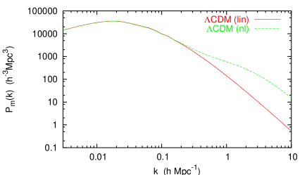
Figure 2: Matter power spectrum $P_{m}(k)$ for a flat fiducial $\Lambda$CDM model defined by $\Omega_{\Lambda}=0.7$, $\Omega_{b}h^{2}=0.019$, $h=0.72$. Linear (solid) and non-linear (dashed) regimes are presented.

V Weak lensing in general relativity

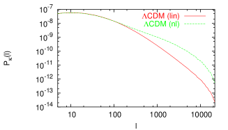
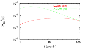
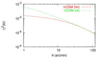
Figure 3: (left) Convergence power spectrum $P_{\kappa}(\ell)$ as a function of the multipole $\ell$ and the 2-point statistics of the shear field: (middle) the aperture mass variance and (right) the shear variance in the case of the fiducial $\Lambda$CDM model (123).

V.1 Generalities

When gravity is described by general relativity, then at late time matter dominates and the anisotropic stresses are negligible so that the two gravitational potentials are equal

$$\phi=\psi$$ (115)

consequently the deflecting potential is simply given by

$$\Phi=2\phi.$$ (116)

On sub-Hubble scales, the gravitational potential is related to the matter density perturbation by the Poisson equation which implies that

$$\delta_{\mathrm{eff}}=\delta_{m},$$ (117)

where $\delta_{m}=\delta\rho_{m}/\rho_{m}$ is the matter density contrast. Let us stress that on large scales, one must take into account the radiation anisotropic stress which will induce a departure from this equality (see Fig. 13). Starting from an initial time, $a_{i}$, where the modes of interest are sub-Hubble, one can decompose the density field as

$$\delta_{m}(\bm{k},a)=D(a)\delta(\bm{k},a_{i})=D(a)\delta_{i}$$ (118)

where $D(a)$ is the growth factor. It follows that $P_{\mathrm{eff}}(k,a)=D^{2}(a)P_{\delta}(k)$. Its equation of evolution, in the Newtonian regime, is given by

$$\ddot{D}+\mathcal{H}\dot{D}-4\pi G\rho_{m}a^{2}D=0.$$ (119)

It can be rewritten by using the redshift as variable as

$$D^{\prime\prime}+\left(\frac{H^{\prime}}{H}-\frac{1}{1+z}\right)D^{\prime}-\frac{3}{2}\Omega_{m,0}(1+z)D=0,$$ (120)

setting $a_{0}=1$ and where a prime refers to a derivative with respect to $z$. This equation has two solutions, a decaying mode, $D\propto H$, and a growing mode

$$D(a)=\frac{5}{2}\frac{H(a)}{H_{0}}\Omega_{m,0}\int_{0}^{a}\frac{\mathrm{d}\tilde{a}}{\left[\tilde{a}E(\tilde{a})\right]^{3}}.$$ (121)

The convergence power spectrum takes the simplified form

$$P_{\kappa}(\ell)=\frac{9H_{0}^{4}}{4}\Omega_{m,0}\int\left[\frac{g(\chi)}{a(\chi)}\right]^{2}P_{\delta}\left[\frac{\ell}{S_{K}(\chi)}\right]D^{2}(\chi)\mathrm{d}\chi.$$ (122)

V.2 $\Lambda$CDM

The power spectrum (122) depends on the cosmological parameters through the growth function and the angular distances and on the normalization of the power spectrum. As emphasized above, we do not perform such a splitting and use the complete expression (95) so that our results depend on the cosmological parameters and the primordial spectrum are CMB-normalized.

As a reference model, we choose a flat $\Lambda$CDM with

$$\Omega_{\Lambda,0}=0.7,\,\,\Omega_{m,0}=0.3,\,\,\Omega_{b,0}=0.037,\,\,h=0.72.$$ (123)

Figure 3 depicts the convergence power spectrum, the aperture mass and the shear variance for a $\Lambda$CDM model. This model will be our reference model and we will try to quantify the deviation from its prediction on various models.

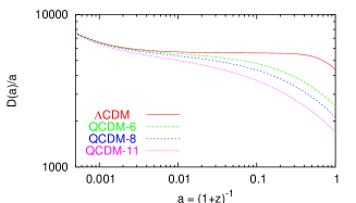
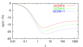
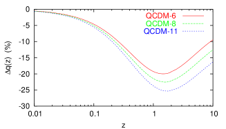
Figure 4: Comparison between the fiducial $\Lambda$CDM model (123) and various quintessence models. (left) the growth factor normalized to its value in an Einstein-de Sitter universe, $D(a)/a$, as a function of the scale factor $a$, normalized at high redshift; (middle) Relative deviation from $\Lambda$CDM on the comoving radial distance, $\chi(z)$, and (right) on the geometrical factor, $q(z)$. In all plots, we consider three QCDM models with potential (124) with $m=6,8,11$ from top to bottom.

V.3 Quintessence: effect of the potential

As a first generalization to the previous $\Lambda$CDM model we consider a class of quintessence models (QCDM) with runaway potentials of the form

$$V(\varphi)=M^{4}\varphi^{-m}.$$ (124)

In the slow-roll regime, the quintessence field acts as a repulsive matter component that replaces the cosmological constant. Gravity is still described by general relativity and the main effects on the lensing observables arise from the modification of the Friedman equations, and thus of the angular distances and of the growth factor of the density field.

To estimate the amplitude of the effects, let us follow Ref. berben and assume that the sources are located at a redshift $z_{s}$ so that the source distribution is simply given by $p(\chi)=\delta(\chi-\chi_{s})$ and thus $g(\chi)=S_{K}(\chi_{s}-\chi)/S_{K}(\chi_{s})$. The function

$$\mathcal{W}(\chi,\chi_{s})\equiv\frac{S_{K}(\chi)S_{K}(\chi_{s}-\chi)}{S_{K}(\chi_{s})a}$$ (125)

is peaked around $\chi_{s}/2$ so that it can be approximated by

$$\mathcal{W}^{2}\simeq\mathcal{W}_{1/2}^{2}\delta(\chi-\chi_{1/2})$$ (126)

with $\chi_{1/2}\simeq\chi_{s}/2$ and

$$\mathcal{W}_{1/2}^{2}=\int_{0}^{\chi_{s}}\mathcal{W}^{2}(\chi,\chi_{s})\mathrm{d}\chi.$$ (127)

Plugging this approximation into Eq. (95) allows to estimate the shear power spectrum as

$$P_{\kappa}(\ell)\sim\frac{9}{4}H_{0}^{2}\Omega_{m,0}\left[\frac{\mathcal{W}_{1/2}}{S_{K}(\chi_{1/2})}\right]^{2}P\left(\frac{\ell}{S_{K}(\chi_{1/2})},\chi_{1/2}\right).$$ (128)

Assuming that the initial power spectrum takes the form

$$P_{\delta}(k)=Ak^{n},$$ (129)

we get that in the linear regime $P_{\rm lin}=D^{2}Ak^{n}$ and $P_{\rm nl}\sim a^{3}Ak^{3(3+n)/2}$ so that Eqs. (111-113) imply that

$$k\sim\left(k_{\rm nl}^{2}/Aa^{2}\right)^{1/(5+n)}.$$ (130)

As long as we are considering modes in the linear regime, the effect of the quintessence field is mainly encoded in the growth function. We get

$$\left.\frac{P_{\kappa}^{Q}}{P_{\kappa}^{\Lambda}}\right|_{\rm lin} \sim \left(\frac{\mathcal{W}_{1/2}^{Q}}{\mathcal{W}_{1/2}^{\Lambda}}\right)^{2}\left(\frac{S^{\Lambda}_{K}(\chi_{1/2}^{\Lambda})}{S^{Q}_{K}(\chi_{1/2}^{Q})}\right)^{2+n}$$ (131)

$$\qquad\qquad\left(\frac{D^{Q}_{1/2}/D^{Q}_{0}}{D^{\Lambda}_{1/2}/D^{\Lambda}_{0}}\right)^{2}\frac{P_{0}^{Q}}{P_{0}^{\Lambda}},$$

where $D_{1/2}$ and $D_{0}$ are the values of the growth factor at $\chi=\chi_{1/2}$ and $\chi_{0}$ respectively and $P_{0}$ i the value of the matter power spectrum today, evaluated at $k=1h\,\mathrm{Mpc}^{-1}$.

In the non-linear regime, the matter power spectra are not distorted in the same way because the same value of $k_{\rm nl}$ does not correspond to the same $k$. It follows that

$$\left.\frac{P_{\kappa}^{Q}}{P_{\kappa}^{\Lambda}}\right|_{\rm nl} \sim \left(\frac{\mathcal{W}_{1/2}^{Q}}{\mathcal{W}_{1/2}^{\Lambda}}\right)^{2}\left(\frac{S^{\Lambda}_{K}(\chi_{1/2}^{\Lambda})}{S^{Q}_{K}(\chi_{1/2}^{Q})}\right)^{2}$$ (132)

$$\qquad\qquad\times\left(\frac{z_{1/2}^{\Lambda}}{z_{1/2}^{Q}}\right)^{3}\left(\frac{P_{0}^{Q}}{P_{0}^{\Lambda}}\right)^{3/(5+n)}$$

if the spectral index is the same in both models. The relations (131) and (132) show that on small scales the shape of the matter power spectrum is modified in quintessence models.

Table 2: Quintessence models (QCDM): background effects. (Upper table) Maximum relative deviation on the comoving radial distance, $\chi(z)$, geometrical factor, $q(z)$, and linear growth factor, $D(z)$, from the fiducial $\Lambda$CDM model for three models with inverse power law potential, Eq. (124). (Lower table) Quantities used to estimate the amplitude of the effects on the weak lensing observable, according to Eq. (131). The amplitude of the matter power spectrum $P_{0}$ is evaluated at $k=1\,h\,\mathrm{Mpc}^{-1}$. For the $\Lambda$CDM model $z_{1/2}\simeq 0.51$, for all the quintessence models $z_{1/2}\simeq 0.48$.

$m$	$\Delta\chi(z)\;(\%)$	$\Delta q(z)\;(\%)$	$\Delta D(z)\;(\%)$
$6$	$-17$ at $(z=3.4)$	$-20$ at $(z=1.4)$	$-42$
$8$	$-19$ at $(z=3.9)$	$-23$ at $(z=1.6)$	$-51$
$11$	$-21$ at $(z=4.7)$	$-26$ at $(z=1.7)$	$-61$

$m$	$\chi_{1/2}/\chi^{\Lambda}_{1/2}$	$\mathcal{W}_{1/2}^{2}/(\mathcal{W}_{1/2}^{2})^{\Lambda}$	$D_{1/2}/D_{0}$	$P_{0}/P^{\Lambda}_{0}$
$6$	$0.853$	$0.611$	$1.052$	$0.275$
$8$	$0.844$	$0.580$	$1.056$	$0.189$
$11$	$0.835$	$0.549$	$1.060$	$0.113$

Table 3: Quintessence models (QCDM): absolute values of the convergence power spectrum, $P_{\kappa}(\ell)$, aperture mass variance, $\langle M_{ap}^{2}(\theta)\rangle$, and shear variance, $\langle\gamma^{2}(\theta)\rangle$ at two angular scales respectively in the linear and non-linear regimes. For the small scales we give both the value in the linear and non-linear regime (values within parenthesis). Each model is labelled by $\mathrm{QCDM}m$, where $m$ defines the inverse power law potential, Eq. (124).

model	$P_{\kappa}(\ell)$		$\langle M_{ap}^{2}(\theta)\rangle$		$\langle\gamma^{2}(\theta)\rangle$
	$\ell=180$	$\ell=7200$	$\theta=2^{\circ}$	$\theta=3^{\prime}$	$\theta=2^{\circ}$	$\theta=3^{\prime}$
$\Lambda\mathrm{CDM}$	$7\times 10^{-9}$	$2\times 10^{-12}\;(4\times 10^{-11})$	$3\times 10^{-6}$	$4\times 10^{-6}\;(5\times 10^{-5})$	$8\times 10^{-6}$	$1\times 10^{-4}\;(3\times 10^{-4})$
$\mathrm{QCDM}6$	$1\times 10^{-9}$	$4\times 10^{-13}\;(6\times 10^{-12})$	$7\times 10^{-7}$	$6\times 10^{-7}\;(6\times 10^{-6})$	$2\times 10^{-6}$	$2\times 10^{-5}\;(4\times 10^{-5})$
$\mathrm{QCDM}8$	$9\times 10^{-10}$	$2\times 10^{-13}\;(3\times 10^{-12})$	$5\times 10^{-7}$	$4\times 10^{-7}\;(3\times 10^{-6})$	$1\times 10^{-6}$	$1\times 10^{-5}\;(2\times 10^{-5})$
$\mathrm{QCDM}11$	$4\times 10^{-10}$	$1\times 10^{-13}\;(1\times 10^{-12})$	$3\times 10^{-7}$	$2\times 10^{-7}\;(1\times 10^{-6})$	$7\times 10^{-7}$	$9\times 10^{-6}\;(1\times 10^{-5})$

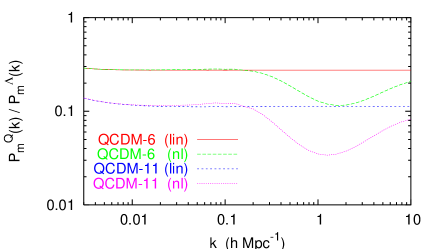
Figure 5: The ratio of the three dimensional power spectrum of the matter perturbation $P_{m}(k)$ of two quintessence models to the reference $\Lambda$CDM model (123) for $m=6$ and $m=11$.

Figure 6: (left) Convergence power spectrum $P_{\kappa}(\ell)$ as a function of the multipole $\ell$ and the 2-point statistics of the shear field: (middle) the aperture mass variance and (right) the shear variance for the reference $\Lambda$CDM model (123) (solid/long-dashed lines) and two quintessence models ($m=6$, short-dashed/dotted line; $m=11$, long-dashed-dotted/short-dashed-dotted line).

As can be seen on Fig. 4, matter perturbations grow more slowly than in a $\Lambda$CDM model. The CMB normalization implies that at lower redshift the amplitude of density perturbations are smaller in quintessence models. Thus, a given scale enters the non-linear regime later than in a $\Lambda$CDM. This time delay accounts for the sharp modification of the spectrum at small wavenumbers. Table 2 gives the order of magnitude of the expected effects on the background quantities, the growth factor and the lensing observables. For instance let us concentrate of a quintessence model with $m=6$. Table 3 shows that the convergence power spectrum is 80% to 85% smaller in quintessence than in $\Lambda$CDM. Now, assume we normalize the power spectra on linear scales at $z=0$, it will have implied to multiply the linear power spectrum by $\sim 7$ and the non-linear one by $\sim\sqrt{7}$. Thus, we would have found that the non-linear regime will differ roughly by 50% from the $\Lambda$CDM. This conclusions are similar to the ones of Ref. berben and show that the change of spectrum between the linear and non-linear part of the spectrum sets strong constraints on the time evolution of the dark energy.

VI Weak lensing in scalar-tensor theories

We now turn to the case where gravity is not described by general relativity but by a scalar-tensor theory.

VI.1 Newtonian regime

Before we discuss explicit models, we can try to evaluate and discuss the expected effects on lensing observables. For that purpose, let us first look at the perturbation equations in the Newtonian regime. We consider modes with wavelengths smaller than the Hubble length and also assume that the scalar field is light.

In the matter era and on sub-Hubble scales, the equation (210) of Appendix B reduces to

$$\psi-\phi=\frac{F_{\varphi}}{F}\delta\varphi,$$ (133)

so that non-minimal coupling induces an extra-contribution to the anisotropic stress, while Eq. (B) reduces to a generalized Poisson equation

$$F\Delta\phi=4\pi G_{*}\rho a^{2}\delta_{m}-\frac{F_{\varphi}}{2}\Delta\delta\varphi.$$ (134)

The evolution equation (208) of the matter field takes the form

$$\dot{\delta}_{m}=-\Delta V+3\dot{\psi}$$ (135)

and the Euler equation (209) to

$$\dot{V}+\mathcal{H}V=-\phi.$$ (136)

This set has to be completed by the Klein-Gordon equation for the scalar field evolution

$$\left(\Delta-U_{\varphi\varphi}a^{2}\right)\delta\varphi=F_{\varphi}\Delta(\phi-2\psi).$$ (137)

VI.2 Effects and amplitudes

Various effects are expected. As in the case of quintessence, the Friedmann equation is modified so that the geometrical function $q$ as well as the growth of density fluctuations are modified.

Besides, there are two specific effects which do not appear in pure quintessence models due to the modification of Einstein equations:

1. The Poisson equation does not take its standard Newtonian form so that

   $$\delta_{\mathrm{eff}}\not=\delta_{m}.$$ (138)

2. The two gravitational potentials are not equal anymore so that

   $$\Phi\not=2\phi.$$ (139)

   By extension to the post-Newtonian formalism, we can define the parameter $\gamma^{\mathrm{PPN}}$ in the cosmological context by

   $$\psi=\gamma^{\mathrm{PPN}}\phi$$ (140)

   so that $\Phi=[1+\gamma^{\mathrm{PPN}}(z)]\phi$.

VI.2.1 Linear regime

The two equations of evolution (135-136) can be combined to get the evolution of the density field

$$\ddot{\delta}_{m}+2\mathcal{H}\delta_{m}-\Delta\phi=3a^{2}\left(\dot{\psi}a^{-2}\right)^{.}.$$ (141)

When $U_{\varphi\varphi}$ is much smaller than the wavelength of the modes we consider then we can combine Eq. (133) and Eq. (137) to get the fluctuation of the scalar field as

$$\delta\varphi\simeq-\frac{FF_{\varphi}}{F+2F_{\varphi}^{2}}\phi.$$ (142)

In particular, this implies that

$$\gamma^{\mathrm{PPN}}(z)-1=\frac{F_{\varphi}^{2}}{F+2F_{\varphi}^{2}}$$ (143)

similarly, as obtained in § II.2 in a non-cosmological context. Inserting Eq. (142) in the generalized Poisson equation (134), one gets

$$\Delta\phi\simeq 4\pi G_{\mathrm{cav}}\rho a^{2}\delta_{m}$$ (144)

where $G_{\mathrm{cav}}$ is defined by Eq. (26) and is indeed time dependent. Using the Eq. (81), this equation implies that

$$\delta_{\mathrm{eff}}\simeq\frac{1}{2}\frac{G_{\mathrm{cav}}(z)}{G_{\mathrm{eff}}(0)}\left[1+\gamma^{\mathrm{PPN}}(z)\right]\delta_{m}\simeq\frac{F_{0}}{F}\left[1+\eta(\varphi)\right]\delta_{m}$$ (145)

where $\eta(\varphi)\equiv 2F_{\varphi}^{2}/(2F+3F_{\varphi}^{2})$. Today $\eta(\varphi_{0})$ is expected to be smaller than a few $10^{-3}$.

The density evolution follows an equation that is similar to the pure Newtonian case but where the gravitational constant has to be replaced by its time dependent value

$$\ddot{\delta}_{m}+\mathcal{H}\dot{\delta}_{m}-4\pi G_{\mathrm{cav}}\rho a^{2}\delta_{m}=0.$$ (146)

If we decompose the density field as in Eq. (118), we obtain that the effective growth factor is

$$D_{\mathrm{eff}}\simeq\frac{F_{0}}{F}\left[1+\eta\right]^{2}D(a)$$ (147)

where $D$ is solution of Eq. (146). Written in terms of the redshift, it takes the form

$$D^{\prime\prime}+\left(\frac{H^{\prime}}{H}-\frac{1}{1+z}\right)D^{\prime}-\frac{3}{2}\Omega_{m,0}(1+z)\frac{G_{\mathrm{cav}}(z)}{G_{\mathrm{eff}}(0)}D=0,$$ (148)

where $\Omega_{m,0}$ is defined by Eq. (198). It follows that the shear power spectrum takes the form

$$P_{\kappa}(\ell) = \frac{9H_{0}^{4}}{4}\Omega_{m,0}\int\left[\frac{g(\chi)}{a(\chi)}\right]^{2}\left(\frac{F_{0}}{F}\right)^{2}\left[1+\eta\right]^{2}$$ (149)

$$\qquad\qquad\times D^{2}(\chi)P_{\delta}\left[\frac{\ell}{S_{K}(\chi)},\chi\right]\mathrm{d}\chi.$$

It follows from this expression that we can estimate $P_{\kappa}$ by solving the background equations solely. In particular, because of the form (144) of the Poisson equation, we do not expect effects as the ones described in Ref. ub00 on small scales (see however Fig. 13).

VI.2.2 Remark on the linear to non-linear mapping

The linear to non-linear mapping procedure has to be extended when working in scalar-tensor theory, in particular because we will have to deal with the scalar field perturbations. As Eq. (95) shows, we must determine $P_{\mathrm{eff}}^{\rm nl}$. For that purpose, we use the definition (81) to define $\delta_{\mathrm{eff}}$ and we decompose it as

$$\delta_{\mathrm{eff}}=\delta_{m}+\delta_{X}$$ (150)

where $\delta_{X}$ contains the contribution of the scalar field perturbation and its derivative.

Assuming that the scalar field does not cluster, as it is the case in quintessence, $\delta_{X}$ will not enter the non-linear regime so that we can assume that

$$\delta_{X}^{\rm nl}=\delta_{X}^{\rm lin}.$$ (151)

In the Newtonian linear regime, Eq. (81) implies that

$$\delta_{\mathrm{eff}}^{\rm lin}=\frac{a/a_{0}}{3H_{0}^{2}\Omega_{m,0}}\Delta\Phi^{\rm lin}.$$ (152)

The output of our CMB code gives access to $\Phi^{\mathrm{lin}}$ and $\delta^{\rm lin}_{m}$ from which we can deduce $\delta_{\mathrm{eff}}^{\mathrm{lin}}$ and thus $\delta_{X}^{\mathrm{lin}}$. With this ansatz, we get the effective perturbation in the non-linear regime

$$\delta_{\mathrm{eff}}^{\rm nl}=\delta_{m}^{\rm nl}+\delta_{X}^{\rm lin}.$$ (153)

It follows that

$$P_{\mathrm{eff}}^{\rm nl}(k,z)=P_{m}^{\rm nl}(k,z)+P_{X}^{\rm lin}(k,z)+2\sqrt{P_{m}^{\rm nl}(k,z)P_{X}^{\rm lin}(k,z)}.$$ (154)

When we are deeply in the Newtonian regime, but still in the linear regime, Eq. (145) implies that $\delta_{X}\rightarrow(F_{0}/F-1)\delta_{m}$ so that

$$P_{\mathrm{eff}}^{\rm lin}(k,z)\longrightarrow\left(\frac{F_{0}}{F}\right)^{2}P_{m}^{\rm lin}(k,z),$$

neglecting the contribution in $\eta$. In fact, notice that the ratio $P^{\rm lin}_{\mathrm{eff}}/P^{\rm lin}_{m}$ evaluated today is always grater than one, because of the non vanishing anisotropic stress of the radiation and non-minimally coupled scalar fields. In the non-linear regime,

$$P_{\mathrm{eff}}^{\rm nl}(k,z)\longrightarrow\left[\sqrt{P_{m}^{\rm nl}(k,z)}+\left(\frac{F_{0}}{F}-1\right)\sqrt{P_{m}^{\rm lin}(k,z)}\right]^{2}$$

so that at $z=0$, $P_{\mathrm{eff}}^{\rm nl}(k)\rightarrow P_{m}^{\rm nl}(k)$, as expected from our assumption that the scalar field does not cluster.

Hence, our ansatz amounts for an interpolation between the super-Hubble regime where the contribution of the scalar field perturbation cannot be neglected and the Newtonian regime where the effective Poisson equation (144) hold. Note that it assumes that the scalar field does not enter the non-linear regime. In fact the mapping procedure of Ref. smithetal uses a halo model and it was shown vdb that in a spherical collapse, the scalar field does indeed not cluster (see also Ref. carlo ; amen1 ). So, we can hope this interpolation to be justified but, at the time being, we have no possibility to check it.

VI.2.3 Effect on the shear power spectrum

Following the approximation of Section V.3, we can compare two models which differ only by the theory of gravity (i.e. same quintessence potential or $\Lambda$CDM models).

In the linear regime, we get

$$\left.\frac{P_{\kappa}^{ST}}{P_{\kappa}^{RG}}\right|_{\rm lin} \sim \left(\frac{\mathcal{W}_{1/2}^{ST}}{\mathcal{W}_{1/2}^{RG}}\right)^{2}\left(\frac{S^{\Lambda}_{K}(\chi_{1/2}^{RG})}{S^{ST}_{K}(\chi_{1/2}^{ST})}\right)^{2+n}\left(\frac{F_{0}}{F(z_{1/2})}\right)^{2}$$ (155)

$$\qquad\qquad\times\left(\frac{D^{ST}_{1/2}/D^{ST}_{0}}{D^{RG}_{1/2}/D^{RG}_{0}}\right)^{2}\frac{P_{0}^{ST}}{P_{0}^{RG}}$$

while in the non-linear regime we obtain

$$\left.\frac{P_{\kappa}^{ST}}{P_{\kappa}^{RG}}\right|_{\rm nl} \sim \left(\frac{\mathcal{W}_{{}_{1/2}}^{ST}}{\mathcal{W}_{{}_{1/2}}^{RG}}\right)^{2}\left(\frac{S^{RG}_{K}(\chi_{{}_{1/2}}^{RG})}{S^{ST}_{K}(\chi_{{}_{1/2}}^{ST})}\right)^{2}\left(\frac{F_{0}}{F(z_{{}_{1/2}})}\right)^{2}$$ (156)

$$\qquad\qquad\times\left(\frac{z_{{}_{1/2}}^{RG}}{z_{{}_{1/2}}^{ST}}\right)^{3}\left(\frac{P_{0}^{ST}}{P_{0}^{RG}}\right)^{3/(5+n)}.$$

The main contribution to the modification of the shear power spectrum, and consequently on the 2-points statistics, is expected to arise from the evolution of the matter power spectrum. Because of the normalization to the CMB, i.e. at high redshift, its amplitude evaluated today accounts for integrated effect over a wide redshift range. Therefore it leaves trace on the shear power spectrum, even if the computation of the shear power spectrum involves an integration just up to the source redshift $z_{s}$. Instead, as for quantities depending on the redshift range $[0,z_{s}]$, eventually evaluated at $z_{1/2}$, their contribution can become relevant only if $z_{1/2}$ is sufficiently high. In particular, for $z_{1/2}\simeq 0.5$ the deviation from general relativity described by $F_{0}/F_{1/2}$ is negligible (see Fig. 7, hence the peculiar effects of scalar-tensor theories are ultimately encoded in the amplitude of the matter power spectrum evaluated today. However notice that, accounting for sources at higher redshift, where the deviations from general relativity could become significant, and looking at lenses at low redshift, one should detect deviation of order 10% on weak-lensing observables, peculiar of a scalar-tensor theory.

VII Investigation of two explicit models

We consider two test models to discuss in more details the amplitude of scalar-tensor theories on lensing observations. Indeed, scalar-tensor theories have two free functions that need to be specified, which open a parameter space much larger than a standard $\Lambda$CDM. Any quintessence model is specified by its potential $U(\varphi)$. To embed it in scalar-tensor theories, one has two possibilities: (1) assume that the potential in Jordan frame, $U(\varphi)$ is the quintessence potential and choose a coupling function $F(\varphi)$ or (2) assume that the potential in Einstein frame, $V(\varphi_{*})$, is the quintessence potential and choose a coupling function $\alpha(\varphi_{*})$. The second possibility is probably more secure from a theoretical point of view since it amounts to specify the property of the true spin-0 degree of freedom of the theory.

We will however investigate the two possibilities. We first consider in § VII.1 the case of a non-minimally coupled scalar field and in § VII.2 the case of scalar-tensor models that incorporate attraction toward general relativity.

Figure 7: Deviation from general relativity parameterized by $\gamma_{\rm PPN}(z)-1$ for several non-minimally coupled models with Ratra-Peebles potential, Eq. (124), as a function of redshift $z$. Solid line (long dashed line): non-minimal coupling, $\xi=+0.001$ and $m=6\;(m=11)$ [potential defined in Jordan frame]. Short dashed line (dotted line): exponential Damour-Nordvedt type coupling, with $\beta=4,B=0.5$ and $m=6\;(m=11)$ [potential defined in Einstein frame]. Horizontal lines: level of the upper bounds measured by gravitational experiment on Solar System scales ($z\sim 0$).

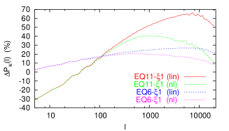
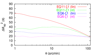
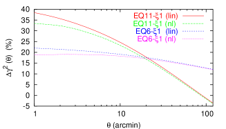
Figure 8: Comparison between an extended quintessence model with $\xi=10^{-2}$ and $m=6$ and a quintessence model with same potential. (left) convergence power spectrum $([P_{\kappa}]_{\rm{EQ}-\xi}/[P_{\kappa}]_{\rm QCDM}-1)$, (middle) aperture mass variance and (right) and shear variance. Solid (long dashed): linear (non-linear) regime for Ratra-Peebles potential with $m=6$. Short dashed (dotted): linear (non-linear) regime for Ratra-Peebles potential with $m=11$.

VII.1 Non-minimally coupled case

We consider the simplest model we can think of for which the coupling of the scalar field to gravity is described by the function

$$F(\varphi)=1+\xi\varphi^{2}.$$ (157)

The constraint (25) implies that

$$\left|\xi\varphi_{0}\right|<0.55\times 10^{-3}.$$ (158)

Generically ru02 , $\varphi_{0}\sim\mathcal{O}(1)$ today so that this constraints implies that

$$\left|\xi\right|\lesssim 0.5\times 10^{-3}.$$ (159)

In this class of models, all deviations from general relativity will scale like $\xi$ so that we expect $\delta P_{\kappa}/P_{\kappa}\sim\mathcal{O}(\xi)$, that is very small effects.

VII.1.1 $\xi\Lambda$CDM: effect of the coupling

To quantify the effect of this coupling, we first assume that $\varphi$ has no potential and that there exists a cosmological constant.

At this point, we should stress that there is no unique way of defining a cosmological constant in scalar-tensor theories. Either one adds this constant in Jordan frame, in which case the associated energy density is constant. But, from Eq. (8), this induces a potential for the true spin-0 degrees of freedom of the theory. On the other hand, one could argue that imposing a constant potential in Einstein frame lets the scalar field massless hence generalizing a constant potential. But, it will not correspond to a constant energy density in the physical (Jordan) frame. Let us also mention that adding a cosmological constant in Jordan frame modifies the potential as $U\rightarrow U+\Lambda$, corresponding to the change $V\rightarrow V+\Lambda A^{4}/2$. It follows that the spin-0 degree of freedom can remain massless only if

$$V^{\prime\prime}(\varphi_{*})+2\Lambda A^{4}(\varphi_{*})\left[4\alpha^{2}+\beta\right]=0.$$

We have considered various models with $U(\varphi)=\Lambda$ and with the constraint $\Omega_{\Lambda}=0.7$ for various value of $\xi$, typically ranging from $-0.005$ to $0.1$. None of them exhibit any departure from the standard $\Lambda$CDM reference model (123), as expected from our general arguments.

VII.1.2 Extended quintessence

We now take into account both effects of a non-minimal coupling and of a runaway potential in Jordan frame. We consider models with $m=6,\,11$ and $\xi=10^{-2},10^{-3},10^{-4},-5\times 10^{-3}$. We will refer to these models by the label $\mathrm{EQ}m-\xi n$, where $m$ stands for the exponent of the runaway potential and $n$ for the value of the coupling ($n=1,\dots,4$ for $\xi=10^{-2}\ldots-5\times 10^{-3}$, respectively).

As expected, the main contribution to the deviation on the shear power spectrum and consequently on the 2-points statistics come from the amplitude of the matter power spectrum evaluated today. The relative differences occurring in the (comoving) angular distance, in the window function and in the growth factor at $z=z_{1/2}\simeq 0.5$ are negligible. Notably, the evolution of the coupling function $F(\varphi)$ is negligible. Anyway, the scaling in $\xi$ is obvious (see Tables 4 and 5).

As can be shown on Fig. 8 we obtain an effect of order 20% for $\xi=0.01$, a value excluded by Solar System constraints, see Fig. 7. For $\xi=10^{-3}$, our results agree with those of Ref. acqua04 . They argue that, taking into account the different normalization of the scalar field compared to our work,

$$\delta P_{\kappa}/P_{\kappa}\sim-16\xi\varphi_{0}^{2},$$

hence leading to a $\sim 2\%$ effect on the shear power spectrum once the constraints (158-159) are taken into account. In general, since the effect scales like $\xi$, we can conclude that for values compatible with Solar System constraints, the amplitude of the effects will be smaller than a percent. Such a low value makes these models, in practice, indistinguishable from their corresponding quintessence models.

VII.2 Attraction toward GR

VII.2.1 Mechanism

Another interesting class of models is the one in which the scalar-tensor theory is attracted toward general relativity today. This feature is better described in Einstein frame. The Klein Gordon equation (cf. Eq. 188) can be rewritten in terms of the new variable

$$p=\ln a_{*}$$ (160)

as

$$\frac{2[1+v(\varphi_{*})]}{3-\varphi_{*}^{{}^{\prime}2}}\varphi_{*}^{\prime\prime}+[1-w+2v(\varphi_{*})]\varphi_{*}^{\prime}=$$

$$\qquad\qquad\quad-\alpha(\varphi_{*})(1-3w)-v(\varphi_{*})\frac{\mathrm{d}\ln V}{\mathrm{d}\varphi_{*}}$$ (161)

where a dash temporarily refers to a derivative with respect to $p$, $w$ refers to the equation of state of all matter fields but $\varphi_{*}$ and where we have introduced the reduced potential

$$v(\varphi_{*})=\frac{V(\varphi_{*})}{4\pi G_{*}\rho_{*}}.$$ (162)

The coupling function $A(\varphi_{*})$ is decomposed as

$$A(\varphi_{*})=\hbox{e}^{a(\varphi_{*})}$$ (163)

so that $\alpha=\mathrm{d}a/\mathrm{d}\varphi_{*}$.

The mechanism of attraction is then well illustrated by the original model dn1 in which the scalar field potential is flat and where $a(\varphi_{*})$ is quadratic. Setting $a(\varphi_{*})=\beta\varphi_{*}^{2}/2$, the Klein-Gordon equation takes the form of the equation of motion of a particle with velocity-dependent inertial mass, $m(\varphi_{*})=2/(3-\varphi_{*}^{{}^{\prime}2})$, subject to a damping force $-(1-w)\varphi_{*}^{\prime}$ in a potential, $(1-3w)a(\varphi_{*})$,

$$\frac{2}{3-\varphi_{*}^{\prime}{}^{2}}\varphi_{*}^{\prime\prime}+(1-w)\varphi_{*}^{\prime}=-\beta(1-3w)\varphi_{*}.$$ (164)

The positivity of the energy implies that $m(\varphi_{*})>0$. During radiation era $w=1/3$ and the field is decoupled from the potential and will tend to a constant value, $\varphi_{*,R}$, whatever its initial velocity. During the matter era, the evolution of $\varphi_{*}$ is the one of a damped oscillator that starts with a vanishing initial velocity. $\varphi_{*}$ will thus moved toward the minimum of $a(\varphi_{*})$ where $\alpha=0$, if $\beta>0$. That is the scalar-tensor theory will become infinitely close to general relativity.

VII.2.2 Massless scalar field models

We first investigate a class of models with a vanishing potential and a quadratic coupling defined in the Einstein frame, as in the original Ref. dn1 . The coupling function takes the form

$$a(\varphi_{*})=a_{m}+\frac{1}{2}\beta(\varphi_{*}-\varphi_{m})^{2}$$ (165)

where $\varphi_{m}$ is the value of the field at minimum. The functions $\alpha$ and $\beta$ defined in Eqns. (13) and (14) are thus given by

$$\alpha(\varphi_{*})=\beta(\varphi_{*}-\varphi_{m}),\qquad\beta(\varphi_{*})=\beta.$$ (166)

The coupling (165) can be rewritten as

$$a(\varphi_{*})=a_{0}+\alpha_{0}(\varphi_{*}-\varphi^{*}_{0})+\frac{1}{2}\beta(\varphi_{*}-\varphi_{0})^{2}$$ (167)

where $\varphi_{0}$ is the value of $\varphi_{*}$ today. Without loss of generality, a redefinition of units allows to reduce to this form

$$a(\varphi_{*})=\frac{1}{2}\beta\varphi_{*}^{2}.$$ (168)

The post-Newtonian constraints (23-24) imply that

$$\alpha_{0}^{2}<10^{-5},\quad-8.5\times 10^{-4}<\alpha_{0}^{2}(1+\beta_{0})<1.5\times 10^{-4}.$$ (169)

A detailed analysis dp of the primordial nucleosynthesis in this particular model also give constraints on $(\alpha_{0},\beta)$.

During the matter era, assuming $\varphi_{*}^{\prime}{}^{2}\ll 3$, the Klein-Gordon equation simplifies to

$$\frac{2}{3}\varphi_{*}^{\prime\prime}+\varphi_{*}^{\prime}+\beta\varphi_{*}=0.$$ (170)

According to the value of $\beta$, it has two different kinds of solutions. For $\beta<3/8$, that is for a small curvature of the coupling,

$$\varphi_{*}(z_{*})=A_{+}(1+z_{*})^{3(1+r)/4}+A_{-}(1+z_{*})^{3(1-r)/4}$$ (171)

where we have set $r=\sqrt{1-8\beta/3}$. The solution compatible with the bound (169) is thus given by

$$\varphi_{*}(z_{*})=\varphi_{0}(1+z_{*})^{3(1-r)/4}.$$ (172)

For $\beta>3/8$, we have damped oscillations around the minimum of $a(\varphi_{*})$

$$\varphi_{*}(z_{*}) = (1+z_{*})^{3/4}\left\{A\cos\left[\frac{3}{4}r\ln(1+z_{*})\right]\right.$$ (173)

$$\qquad\left.+B\sin\left[\frac{3}{4}r\ln(1+z_{*})\right]\right\}.$$

In this situation, $G_{\mathrm{cav}}$ may be oscillating during the matter era. In the radiation era, the solution for the scalar field can be shown dn1 to behave as

$$\varphi_{*}=\pm\sqrt{3}\,\mathrm{arctanh}\sqrt{1-A(1+z)^{-2}}+B.$$ (174)

Figure 9: Evolution of the scalar field in Einstein-frame in a model of massless dilaton with a quadratic coupling ($\alpha_{0}=10^{-4}$, $\beta=10^{2}$). We compare the case of a vanishing potential (solid) and a constant potential (dash). The solutions differ only recently. The period of the oscillation is compatible with the analytic result, as can be seen on the left plot where $\varphi_{*}$ has been divided by the damping dactor $(1+z_{*})^{3/4}$.

In figure 9, we show that the numerically computed evolution of the scalar field fits very well the previous analytic solutions. Interestingly, the models considered in Fig. 9 are compatible with nucleosynthesis and Solar System bounds. We can check that the oscillation of the scalar field do not leave any imprint on both matter and CMB angular power spectra.

Figure 10: Relative deviation $(P_{\kappa}/[P_{\kappa}]_{\rm SCDM}-1)$ from a SCDM model ($\Lambda=0$) on the convergence power spectrum of the massless scalar fields models, with quadratic coupling with $(\alpha_{0}^{2},\beta)=(10^{-4},0.1)$, as a function of the multipole $\ell$. Linear (solid) and non-linear (dashed) regime are presented. The field is attracted rapidly toward the minimum of the coupling function so that the model does not differ from a SCDM by more than 0.1%.

Figure 10 depicts the shear power spectrum for a model with a massless dilaton with quadratic coupling (165) with $(\alpha_{0}^{2},\beta)=(10^{-4},0.1)$. The scalar field is attracted toward the minimum of the coupling very efficiently so that the model can hardly be differentiated from the analogous model in general relativity. We emphasize this class of models, which have also been constrained by BBN dp , do not account for the late acceleration of the universe. Thus, we have compared them to a standard cold dark matter model with $\Lambda=0$.

Note that adding a constant potential, that is a cosmological constant defined in Einstein frame, lets the dilaton massless and does not affect its dynamics apart from at very small redshift (see Fig. 9).

As for non-minimal quadratic model, this class of model will not leave any significant signature on lensing observables.

VII.2.3 Extended quintessence

In the previous models, the scalar field accounts for a new interaction but not for the acceleration of the universe that was driven by a pure cosmological constant.

In the context of quintessence, extended quintessence models have been widely considered. In particular, it was realized bp that scalar-tensor quintessence models with attraction toward general relativity can be constructed. This is the case for instance when quintessence is constructed as a runaway dilaton runaway1 ; runaway2 . In this case, the coupling function typically reduces to

$$\alpha(\varphi_{*})=-B\hbox{e}^{-\beta\varphi_{*}}$$ (175)

and the potential takes the form

$$V(\varphi_{*})=M_{*}^{4}\varphi_{*}^{-m}.$$ (176)

During radiation era, the coupling is not effective and the scalar field evolution will get its standard attractor solution. In the matter era, the field will start by slow rolling. If we assume it is always slow-rolling and that it explains the acceleration of the universe today, then the Klein-Gordon equation reduces to

$$\varphi_{*}^{\prime}\simeq B\hbox{e}^{-\beta\varphi_{*}}$$ (177)

whose solution is well approximated by

$$\hbox{e}^{\beta\varphi_{*}}=\hbox{e}^{\beta\varphi_{0}}+B\beta\ln(1+z_{*}).$$ (178)

It follows that

$$\alpha(z_{*})=\frac{\alpha_{0}}{1-\beta\alpha_{0}\ln(1+z_{*})}$$ (179)

where $\alpha_{0}=-B\hbox{e}^{-\beta\varphi_{0}}$ and $\beta_{0}=-\beta\alpha_{0}$. Besides, as in quintessence, the value of $\varphi_{0}$, is obtained from the constraint on $\Omega_{\Lambda}$. Note also that no clear bounds from BBN but the general ones (31) have been inferred. Another constraint on $\varphi^{\prime}_{0}$ arises from the bounds on the time variation of the gravitational constant.

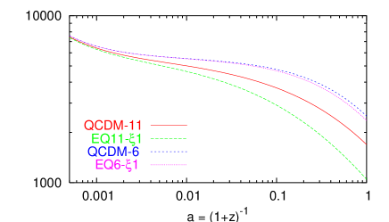
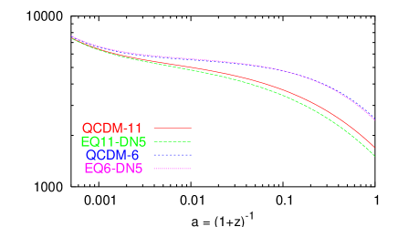
Figure 11: Ratio $D(a)/a$ as a function of the scale factor $a$, normalized at high redshift, for extended quintessence models with quadratic ($\xi=+0.01$, left panel) and exponential coupling ($\beta=4,B=0.1$, right panel) and for the corresponding minimally coupled models. Notice that the potential are defined in different frame.

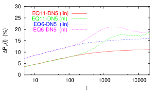
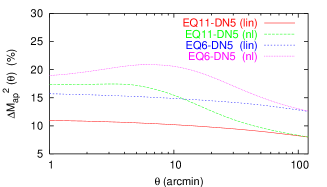
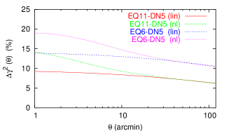
Figure 12: Comparison between an runaway dilaton model with $\beta=4,B=0.1$ and $m=6,11$ and a quintessence model with same potential. (left) convergence power spectrum $([P_{\kappa}]_{\rm{EQ}-\xi}/[P_{\kappa}]_{\rm QCDM}-1)$, (middle) aperture mass variance and (right) and shear variance. Solid (long dashed): linear (non-linear) regime for Ratra-Peebles potential with $m=6$. Short dashed (dotted): linear (non-linear) regime for Ratra-Peebles potential with $m=11$.

Table 4: Extended quintessence models: background effects with respect to the corresponding minimally coupled (QCDM) models (according to § VI.2.3). The models are labeled by $\mathrm{EQ}m-\xi/\mathrm{DN}\,n$, the number $m$ defining the inverse power law potential, Eq. (124), $\xi/\mathrm{DN}$ standing for the (quadratic) non-minimal coupling in Jordan frame or for the exponential Damour-Nordvedt type coupling in Einstein frame, and $n$ singling out the specific model, namely the couplings parameters (see text). For the models $\mathrm{EQ}6-\xi 4$ and $\mathrm{EQ}11-\xi 1$it is $z_{1/2}\simeq 0.49$ and $z_{1/2}\simeq 0.47$, respectively; otherwise it is $z_{1/2}\simeq 0.48$.

model	$\chi_{1/2}/\chi^{Q}_{1/2}$	$\mathcal{W}_{1/2}^{2}/(\mathcal{W}_{1/2}^{2})^{Q}$	$(D_{1/2}/D_{0})/(\cdots)^{Q}$	$P_{0}/P^{Q}_{0}$	$F_{0}/F_{1/2}$
$\mathrm{EQ}6-\xi 1$	$1.021$	$1.031$	$1.006$	$1.114$	$1.0387$
$\mathrm{EQ}6-\xi 2$	$1.000$	$0.994$	$1.000$	$1.008$	$1.0032$
$\mathrm{EQ}6-\xi 3$	$1.000$	$0.999$	$1.000$	$1.005$	$1.0003$
$\mathrm{EQ}6-\xi 4$	$1.031$	$0.011$	$0.989$	$0.982$	$0.0985$
$\mathrm{EQ}6-\mathrm{DN}4$	$1.005$	$1.055$	$1.020$	$2.101$	$1.0081$
$\mathrm{EQ}6-\mathrm{DN}5$	$1.000$	$1.002$	$1.004$	$1.135$	$1.0015$
$\mathrm{EQ}11-\xi 1$	$1.005$	$1.066$	$1.044$	$1.211$	$1.0807$
$\mathrm{EQ}11-\xi 2$	$1.000$	$0.989$	$1.002$	$1.006$	$1.0060$
$\mathrm{EQ}11-\xi 3$	$1.000$	$0.999$	$1.000$	$1.000$	$1.0006$
$\mathrm{EQ}11-\xi 4$	$1.029$	$1.116$	$0.980$	$0.994$	$0.0975$
$\mathrm{EQ}11-\mathrm{DN}4$	$1.000$	$1.003$	$1.027$	$1.727$	$1.0026$
$\mathrm{EQ}11-\mathrm{DN}5$	$1.000$	$1.000$	$1.005$	$1.099$	$1.0004$

Table 5: Extended quintessence models: maximum deviation on the convergence power spectrum, $\Delta P_{\kappa}(\ell)$, aperture mass variance, $\Delta\langle M_{ap}^{2}(\theta)\rangle$, and shear variance, $\Delta\langle\gamma^{2}(\theta)\rangle$, from the corresponding minimally coupled models (QCDM). Every weak lensing observable is evaluated at two angular scales and the effects of the linear and non-linear regime (values within parenthesis) are accounted for. In second and third column, deviation from general relativity parametrized by $\gamma^{\mathrm{PPN}}(z)-1$, Eq. (17), is quoted. Model labeled as in table (4).

model	$(\gamma^{\mathrm{PPN}}-1)\times 10^{-3}$		$\Delta P_{\kappa}(\ell)\;(\%)$		$\Delta\langle M_{ap}^{2}(\theta)\rangle\;(\%)$		$\Delta\langle\gamma^{2}(\theta)\rangle\;(\%)$
	$z=0$	$z=1$	$\ell=180$	$\ell=7200$	$\theta=2^{\circ}$	$\theta=3^{\prime}$	$\theta=2^{\circ}$	$\theta=3^{\prime}$
$\mathrm{EQ}6-\xi 1$	$140$	$105$	$20$	$27\;(16)$	$18$	$27\;(18)$	$12$	$19\;(21)$
$\mathrm{EQ}6-\xi 2$	$1.6$	$1.0$	$1.8$	$2.2\;(0.8)$	$\lesssim 2$	$\sim 2\;(1)$	$1$	$\lesssim 2\;(\lesssim 1)$
$\mathrm{EQ}6-\xi 3$	$1.5\times 10^{-2}$	$0$	$0.7$	$0.7\;(0.7)$	$0.6$	$\lesssim 0.7\;(\lesssim 0.7)$	$<0.6$	$\lesssim 0.7\;(0.8)$
$\mathrm{EQ}6-\xi 4$	$31$	$20$	$4$	$8\;(2)$	$4$	$\lesssim 8\;(\lesssim 2)$	$4\;(2)$	$6\;(2)$
$\mathrm{EQ}6-\mathrm{DN}4$	$5.3$	$125$	$107$	$133\;(165)$	$98$	$130\;(176)$	$79$	$110\;(154)$
$\mathrm{EQ}6-\mathrm{DN}5$	$0.27$	$0.61$	$14$	$\lesssim 16\;(19)$	$13$	$16\;(19)$	$11$	$14\;(19)$
$\mathrm{EQ}11-\xi 1$	$312$	$293$	$27$	$32\;(66)$	$18$	$63\;(35)$	$4$	$33\;(31)$
$\mathrm{EQ}11-\xi 2$	$4.4$	$3.3$	$1.8$	$3.2\;(0.3)$	$\lesssim 2$	$3\;(\lesssim 1)$	$0$	$\lesssim 2\;(\lesssim 1)$
$\mathrm{EQ}11-\xi 3$	$4.2\times 10^{-2}$	$0$	$0.1$	$0.3\;(-0.1)$	$0.1$	$\lesssim 0.2\;(-0.1)$	$<0.1$	$\lesssim 0.2\;(0)$
$\mathrm{EQ}11-\xi 4$	$67$	$51$	$4\;(18)$	$11\;(15)$	$5\;(20)$	$11\;(14)$	$0\;(26)$	$7\;(17)$
$\mathrm{EQ}11-\mathrm{DN}4$	$0.32$	$0.83$	$59$	$77\;(129)$	$54$	$75\;(133)$	$41$	$61\;(88)$
$\mathrm{EQ}11-\mathrm{DN}5$	$1.6\times 10^{-2}$	$4.9\times 10^{-2}$	$9$	$11\;(17)$	$8$	$11\;(17)$	$6$	$9\;(14)$

To illustrate this scenario, we consider four flat quintessence models with $\Omega_{\varphi,0}=0.7$, runaway potential (176) with $m=6,11$ and

1. $B=0.5$, $\beta=4$, labelled by DN4;

2. $B=0.1$, $\beta=4$, labelled by DN5.

The two choices of the coupling parameters are chosen to satisfy the “old” Solar System and “new” Cassini constraints, respectively. These models are labelled by $\mathrm{EQ}m-\mathrm{DN}n$, where $m$ defines the inverse power law potential and $n=4,5$. We have to stress that the deviations on BBN constraints for such a class of models need to be studied.

We compare each model with its related quintessence model. Figure 11 depicts the effect of the coupling on the growth of density perturbations. As can be shown on Fig. 12, this implies effects of more than 10% on the shear power spectrum and thus on all the 2-point statistics. On the scales of interest, we can safely use the relations quoted in § VI.2.3. Tables 4 and 5 show that the amplitude of the matter power spectrum evaluated today is the main source of deviation on $P_{\kappa}$. Indeed this amplitude takes into account the whole history of the modes since the CMB, and in particular in eras where large deviations from general relativity are now possible, see Fig. 7. Interestingly, in the shallow universe, deviations from general relativity are small and effect on the background quantity around $z_{1/2}\simeq 0.5$ are of the order of a couple of percents. The comparison of the number presented in tables 4 and 5 with the estimate (155) in the linear regime agrees within a factor of a few percent.

For instance, the model labelled by $\mathrm{EQ}11-\mathrm{DN}5$ fits the Solar System (Cassini) constraints and lead to a deviation of order 10% from the corresponding minimally coupled (QCDM) model on the shear power spectrum.

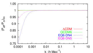
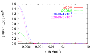
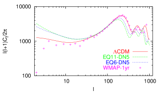
Figure 13: Other possible signatures of the runaway dilaton models. (left) The spectrum of the density perturbation $P_{m}$ differs from the power spectrum of the metric perturbation because of the modification of the Poisson equation. The lensing is sensitive to the deflecting potential $\Phi$ and thus enable to measure $\delta_{\mathrm{eff}}$ (Eq. 81). (middle) The anisotropic stress has two contributions (see Eq; 210) that are important only on large scales, the ansiotropic stress of the radiation and the contribution of the scalar field. The latter is dominant by a large factor in scalar-tensor theories. (right) The WMAP data (cross) compared to the runaway dilaton model prediction assuming an optical depth of $\tau=0.16$. for $m=11$ (dash) and $m=6$ (dot) compared to a $\Lambda$CDM.

Besides, there are other signatures of these models described in Fig. 13. First, the Poisson equation differs from its standard expression since the scalar field, which is a dark component contributes to the total energy density. This implies that $\delta_{\mathrm{eff}}\not=\delta_{m}$. Indeed on small scales we have found that they are proportional [see Eq. (144)] and that the proportionality factor is $k$-independent. This is not the case on large scales anymore. This implies that the shape of $P_{m}$ and $P_{\mathrm{eff}}$ will differ on small $k$. Lensing is sensitive to $P_{\mathrm{eff}}$ while galaxy catalog may determine $P_{m}$. This effect is of order 10% and can be hoped to be detected, as first pointed out in Ref. ubpoisson . Second, in this model the CMB angular power spectrum will be modified: the integrated Sachs-Wolfe effect will be amplified and the amplitude of the secondary peaks will be smaller.

Note however than on large angular scales, $P_{\mathrm{eff}}\not=P_{m}$ even for a pure $\Lambda$CDM model (Fig. 13). The reason is that on these scales, one cannot neglect the anisotropic stress of the radiation (see Eq. 210). Even if the contribution of the scalar field involves a deviation from the usual Poisson equation, it is not clear that this effect is not blurred by the effect of the radiation.

VIII Discussion and conclusions

We have investigated the imprint of quintessence models, both in general relativity and scalar-tensor theories, on weak lensing observations.

For that purpose, we have derived the lensing quantities in a way that does not assume general relativity. Then, we have developed a numerical extension to our CMB code ru02 that computes the shear and convergence statistics. This allows us to “CMB normalize” all spectra.

We have investigated various models and reach different conclusions:

1. Concerning quintessence models, density perturbations grow more slowly than in a $\Lambda$CDM model. This imply some difference of about 10%-20% in the linear regime that can be amplified to more than 50% in the non-linear regime, affecting both the shape and amplitude of the spectra. This conclusion was reached in various previous investigations.

2. For scalar-tensor gravity we have shown that, given the constraints in the Solar System, a non-minimal quadratic coupling in Jordan frame will not change the prediction by more than 1%.

3. On the other hand, runaway dilaton models that incorporate attraction toward general relativity can lead, for the same scalar field potential, to change of order 10% in the predictions. Besides the effect on the amplitude, there exists a differential effect which modifies the shape of the spectra. This opens some hope to be able track such a coupling.

To illustrate the effect on the growth of density perturbations, one can look at the value of $\sigma_{8}$, see table 6. Let us also note that the redshift dependence of the source distribution plays an important role.

There are however some hypothesis and limitations of our analysis that have to be stressed. First, while investigating the non-linear regime, we have adopted universal mappings. These mappings are calibrated on $N$-body simulations for $\Lambda$CDM models. We have argued that these mappings should hold for quintessence models and in scalar-tensor theories, as long as we do not enter the strong field regime. The verification of this hypothesis will require devoted numerical simulation but we do not expect the order of magnitude of the effects discussed here to change drastically.

A second point to be mentioned is related to the possibility that our universe has been reionized. Reionization affects the global normalization of the CMB anisotropies and thus our normalization of the density parameters. As an example of its effect, table 6 compares the results for vanishing optical depth (upper) and for an optical depth $\tau=0.16$. Generically it changes the value of $\sigma_{8}$ by 10% to 20%. But, it will not change the shape of the power spectra. The effect of the reionization on the normalization can easily been understood by looking at the CMB angular power spectrum (Fig. 14).

Let us also emphasize an effect that may be of importance while interpreting lensing data on large scale, as could be obtained by a wide field imager. The radiation anisotropic stress of the radiation implies, even if gravity is described by General Relativity, that the two gravitational potentials are not equal so that the value of the deflecting potential is not equal to twice the gravitational potential.

Weak lensing observables combine the effects of the background properties and the growth of the perturbations and extend from the linear to non-linear regime. These two regimes are complementary mainly because of the sensitivity on the time at which the modes enter the non-linear regime. In conclusion weak lensing survey appear to be a key observation of the shallow universe to investigate the nature of the dark energy.

Table 6: Root mean square of the variance of the matter density contrast on scale of $8h^{-1}$Mpc today, $\sigma_{8}$, assuming vanishing optical depth (upper) or accounting for the reionization with optical depth $\tau=0.16$ (lower).

coupling	$m=0$	$m=6$	$m=8$	$m=11$
no	$0.90$	$0.50$	$0.41$	$0.32$
$\xi 1$	$0.95$	$0.57$	-	$0.40$
$\xi 2$	$0.95$	$0.50$	-	$0.32$
$\xi 3$	-	$0.50$	-	$0.32$
$\xi 4$	$0.95$	$0.48$	-	$0.31$
DN1	$0.83$	-	-	-
DN2	$0.83$	-	-	-
DN3	$0.83$	-	-	-
DN4	-	$0.71$	-	$0.40$
DN5	-	$0.53$	-	$0.33$
no	$1.11$	$0.58$	$0.48$	$0.37$
$\xi 1$	$1.11$	$0.67$	-	$0.47$
$\xi 2$	$1.11$	$0.58$	-	$0.37$
$\xi 3$	-	$0.58$	-	$0.37$
$\xi 4$	$1.11$	$0.56$	-	$0.36$
DN1	$0.96$	-	-	-
DN2	$0.96$	-	-	-
DN3	$0.96$	-	-	-
DN4	-	$0.82$	-	$0.46$
DN5	-	$0.62$	-	$0.39$

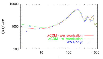
Figure 14: CMB angular power spectra: the WMAP data (cross) compared to two models differing only by their optical depth $\tau=0$ (solid) and $\tau=0.16$ (dash). This shows the influence of the reionization when one chooses to normalize to the CMB temperature anisotropies.

Acknowledgements: CS is partially supported by the Marie Curie programme “Improving the Human Research Potential and the Socio-economic Knowledge Base” under contract n. HMPT-CT-2000-00132. We thank K. Benabed, F. Bernardeau, G. Esposito-Farèse, Y. Mellier, S. Prunet, I. Tereno, L. van Waerbeke for discussions. JPU dedicates this work to Tamara.

Appendix A Background equations

We summarize the equation of the background for the Lagrangian (1) following the general equations presented in Ref. ru02 . The metric takes the form

$$\mathrm{d}s^{2}=a^{2}(\eta)\left[-\mathrm{d}\eta^{2}+\gamma_{ij}\mathrm{d}x^{i}\mathrm{d}x^{j}\right]$$ (180)

and we denote the derivation with respect to the conformal time $\eta$ by a dot and we define the comoving Hubble parameter by

$${\cal H}\equiv\dot{a}/a.$$ (181)

Let us start by the conservation equations. The Klein-Gordon equation for the scalar field takes the form

$$\ddot{\varphi}+2\mathcal{H}\dot{\varphi}=-a^{2}U_{,\varphi}+3F_{,\varphi}\left(\mathcal{H}^{2}+\dot{\mathcal{H}}+K\right)$$ (182)

while the conservation equation of the matter fields is given by

$$\dot{\rho}+3\mathcal{H}(\rho+P)=0.$$ (183)

We have used the notation

$$F_{,\varphi}=\frac{\mathrm{d}F}{\mathrm{d}\varphi}.$$ (184)

Note that the matter energy density scales as $\rho\propto a^{-3}$. This is one of the reasons for which it easier to solve the system in Jordan frame since in Einstein frame $\rho_{*}=A^{4}\rho$ will behave as $A[\varphi_{(}a_{*})]a_{*}^{-3}$ which entangles the evolution of the density with the one of the background.

The Einstein equations give the two Friedmann equations

$$3F\left(\mathcal{H}^{2}+K\right) = 8\pi G_{*}a^{2}\rho+\frac{1}{2}\dot{\varphi}^{2}$$ (185)

$$+a^{2}U-3\mathcal{H}F_{,\varphi}\dot{\varphi}$$

$$2F\left(\mathcal{H}^{2}-\dot{\mathcal{H}}+K\right) = 8\pi G_{*}a^{2}(\rho+P)+\dot{\varphi}^{2}$$ (186)

$$+ F_{,\varphi\varphi}\dot{\varphi}^{2}+F_{,\varphi}\left(\ddot{\varphi}-2\mathcal{H}\dot{\varphi}\right).$$

For completeness, let us give the analog equations in Einstein frame where the metric takes the form

$$\mathrm{d}s_{*}^{2} = a_{*}^{2}(\eta)\left[-\mathrm{d}\eta+\gamma_{ij}\mathrm{d}x^{i}\mathrm{d}x^{j}\right].$$ (187)

The Klein-Gordon equation takes the form

$$\ddot{\varphi}_{*}+2\mathcal{H}_{*}\dot{\varphi}_{*}=-a^{2}_{*}V_{,\varphi}-4\pi G_{*}\alpha(\varphi_{*})(\rho_{*}-3P_{*})$$ (188)

and the Friedmann equations become

$$3\left(\mathcal{H}^{2}_{*}+K\right) = 8\pi G_{*}a_{*}^{2}\rho_{*}+\dot{\varphi}^{2}_{*}+2Va_{*}^{2}$$ (189)

$$3\dot{\mathcal{H}}_{*} = -4\pi G_{*}a^{2}(\rho_{*}+3P_{*})$$ (190)

$$\qquad-2\dot{\varphi}^{2}_{*}+2Va_{*}^{2}.$$

The scale factors of the Jordan and Einstein metrics are related by

$$a=A(\varphi_{*})a_{*}$$ (191)

so that the two cosmic times are related by

$$\mathrm{d}t=A(\varphi_{*})\mathrm{d}t_{*},\qquad\mathrm{d}\eta=\mathrm{d}\eta_{*}.$$ (192)

This implies that redshifts in both frames are related by

$$1+z=\frac{A(\varphi_{*})}{A(\varphi_{*}^{0})}(1+z_{*})$$ (193)

and that the physical length associated with to a comoving length $\ell_{c}$ are connected by

$$\ell^{\rm phys}_{*}=\frac{A(\varphi_{*}^{0})}{A(\varphi_{*})}\ell^{\rm phys}.$$ (194)

It will be convenient to decompose the energy-density of the scalar field as

$$\rho_{\varphi}=\rho_{\rm MC}+\rho_{\rm F}$$ (195)

with

$$\rho_{\rm MC}a^{2} = \frac{1}{2}\dot{\varphi}^{2}+a^{2}U,$$ (196)

$$\rho_{\rm F}a^{2} = -3\mathcal{H}F_{\varphi}\dot{\varphi}.$$ (197)

Then, we can define the density parameters as

$$\Omega_{f}=\frac{8\pi G_{\mathrm{eff}}\rho_{f}a^{2}}{3\mathcal{H}^{2}},\quad\Omega_{\varphi}=\frac{\rho_{\varphi}a^{2}}{3F\mathcal{H}^{2}},\quad\Omega_{K}=-\frac{K}{\mathcal{H}^{2}}$$ (198)

so that the the Friedman equations takes the form

$$\sum_{f}\Omega_{f}+\Omega_{\varphi}+\Omega_{K}=1.$$ (199)

Note that we could have defined

$$\bar{\Omega}_{X}=\frac{8\pi G_{\mathrm{eff},0}\rho_{X}a^{2}}{3\mathcal{H}^{2}},\quad\bar{\Omega}_{\varphi}=\frac{\rho_{\varphi}a^{2}}{3F_{0}\mathcal{H}^{2}},\quad\bar{\Omega}_{K}=-\frac{KF}{\mathcal{H}^{2}F_{0}}.$$ (200)

The two sets of density parameters agrees today and are related by

$$\bar{\Omega}=\Omega F/F_{0}.$$ (201)

We deduce that in a matter universe the Friedmann equation can be rewritten as

$$\frac{{\cal H}^{2}}{{\cal H}^{2}_{0}}=\Omega_{m,0}\frac{F_{0}}{F}(1+z)+\Omega_{\varphi,0}\frac{F_{0}}{F}\frac{\rho_{\varphi}}{\rho_{\varphi,0}}(1+z)^{-2}-\Omega_{K,0}$$ (202)

To finish, let us define the function

$$E(z)=(1+z){\cal H}(z)/{\cal H}_{0}$$ (203)

that is explicitly given by

$$E^{2}=\Omega_{m,0}\frac{F_{0}}{F}(1+z)^{3}+\Omega_{\varphi,0}\frac{F_{0}}{F}\frac{\rho_{\varphi}}{\rho_{\varphi,0}}-\Omega_{K}^{0}(1+z)^{2}.$$ (204)

Appendix B Perturbation equation

The general gauge invariant perturbation equations in scalar-tensor that are being integrated in the CMB code have been presented in Ref. ru02 . We just summarize the scalar mode equations in the case of a single fluid in a universe with Euclidean spatial sections.

In Newtonian gauge, the metric takes the form

$$\mathrm{d}s^{2}=a^{2}(\eta)\left[-(1+2\phi)\mathrm{d}\eta^{2}+(1-2\psi)\mathrm{d}\bm{x}^{2}\right].$$ (205)

The fluid velocity perturbation is decomposed as

$$\delta u_{\mu}=a(-\phi,\partial_{k}V).$$ (206)

$\delta^{\rm N}$ is the density perturbation in Newtonian gauge and we introduce the density perturbation in comoving gauge as

$$\delta=\delta^{\rm N}-3{\cal H}(1+w)V$$ (207)

where $w=P/\rho$.

The fluid conservation equation is given by

$$\left(\frac{\delta^{\rm N}}{1+w}\right)^{.}=-\Delta V+3\dot{\psi}-3{\cal H}\frac{w}{1+w}\Gamma$$ (208)

while the Euler equation takes the form

$$\dot{V}+\mathcal{H}V=-\phi-\frac{c_{s}^{2}}{1+w}\delta+\frac{w}{1+w}\left[\Gamma+\frac{2}{3}\Delta\bar{\pi}\right]$$ (209)

where $c_{s}^{2}=\mathrm{d}P/\mathrm{d}\rho$. $\Gamma$ is the entropy perturbation and $\bar{\pi}$ the anisotropic stress.

Among the four independent Einstein equations, we can retain

$$\psi-\phi=8\pi G_{*}P\bar{\pi}+\frac{F_{\varphi}}{F}\delta\varphi,$$ (210)

$$2F(\dot{\psi}+\mathcal{H}\phi)+\dot{F}\phi = -8\pi G_{*}\rho(1+w)a^{2}V$$ (211)

$$+\dot{\varphi}\delta\varphi+\delta\dot{F}-\mathcal{H}\delta F,$$

$$2F{\Delta}\phi+(\dot{\varphi}^{2}-3\mathcal{H}\dot{F})\phi-3\dot{F}\dot{\phi}$$

$$\qquad=8\pi G_{*}\rho a^{2}\delta-8\pi G_{*}P{\Delta}\bar{\pi}$$

$$\qquad-F_{\varphi}\left[{\Delta}+3\left(\mathcal{H}^{2}+\frac{\dot{F}^{2}}{F^{2}}\right)\right]\delta\varphi$$

$$\qquad+\left(U_{\varphi}a^{2}+3\mathcal{H}\dot{\varphi}\right)\delta\varphi+\dot{\varphi}\delta\dot{\varphi}+3\frac{\dot{F}}{F}\delta\dot{F}.$$ (212)

The Klein-Gordon equation for the evolution of the the scalar field is then given by

$$\delta\ddot{\varphi}+2\mathcal{H}\delta\dot{\varphi}-\left[{\Delta}+3\dot{\mathcal{H}}F_{\varphi\varphi}-U_{\varphi\varphi}a^{2}\right]\delta\varphi\qquad$$

$$\qquad=(\dot{\phi}+3\dot{\psi})\delta\dot{\varphi}-2a^{2}\phi U_{\varphi}$$

$$\qquad-\left[{\Delta}(\phi-2\psi)+3(\ddot{\psi}+3\mathcal{H}\dot{\psi}+\mathcal{H}\dot{\phi})\right]F_{\varphi}.$$ (213)

In all these equations, we have

$$\dot{F}=F_{\varphi}\delta\dot{\varphi},\qquad\ddot{F}=F_{\varphi\varphi}\dot{\varphi}^{2}+F_{\varphi}\delta\ddot{\varphi},\qquad\delta F=F_{\varphi}\delta\varphi.$$

References

• (1) P.J.E Peebles and B. Ratra, Rev. Mod. Phys. 75 (2003) 559; V. Sahni and A. Starobinsky, Int. G. Mod. Phys. D 9 (2000) 373; S.M. Carroll, Living Rev. Rel. 4 (2001) 1.
• (2) J.P. Uzan, N. Aghanim, and Y. Mellier, Phys. Rev. D 70 (2004) 083533.
• (3) C. Wetterich, Nuc. Phys. B 302 (1988) 668; B. Ratra and P.J.E Peebles, Phys. Rev. D 37 (19 88) 3406; R.R. Caldwell, R. Dave and P. J. Steinhardt, Phys.Rev.Lett. 80 (1998) 1582; P.J. Steinhardt, L. Wang, and I. Zlatev, Phys. Rev. D 59 (1999) 023509.
• (4) C. Wetterich, Phys. Lett. B 561 (2003) 10.
• (5) J.-P. Uzan, Rev. Mod. Phys. 75 (2002) 403; J.-P. Uzan, [arXiv:astro-ph/0409424].
• (6) J.-P. Uzan, Phys. Rev. D 59 (1999) 123510.
• (7) T. Chiba, Phys. Rev. D 60 (1999) 083508; L. Amendola, Phys. Rev. D 62 (2000) 043511; A. Riazuelo and J.-P. Uzan, Phys. Rev. D 62 (2000) 083506.
• (8) F. Perrotta, C. Baccigalupi, and S. Matarrese, Phys. Rev. D 61 (2000) 023507.
• (9) A. Riazuelo and J.-P. Uzan, Phys. Rev. D 66, 023525 (2002).
• (10) X. Chen and M. Kamionkowsky, Phys. Rev. D 60 (1999) 104036.
• (11) C. Baccigalupi, S. Matarrese, and F. Perrotta, Phys. Rev. D 62 (2000) 123510.
• (12) L. Amendola, Phys. Rev. Lett. 86 (2001) 196.
• (13) N. Bartolo and M. Pietroni, Phys. Rev. D 61 (2000) 023518.
• (14) G. Esposito-Farèse and D. Polarski, Phys. Rev. D 63, 063504 (2001).
• (15) T. Damour and K. Nordtvedt, Phys. Rev. Lett. 70 (1993) 2217.
• (16) T. Damour and B. Pichon, Phys. Rev. D 59 (1999) 123502.
• (17) C. Will Theory and experiments in gravitational physics (Cambridge University Press, Cambridge, England, 1993); C. Will Living Rev. Rel. 4 (2001) 4.
• (18) M. Gasperini, F. Piazza, and G. Veneziano, Phys. Rev. D65 (2002) 023528.
• (19) T. Damour, F. Piazza, and G. Veneziano, Phys. Rev. D 66 (2002) 081601.
• (20) T. Damour and G. Esposito-Farèse, Class. Quant. Grav. 9 (1992) 2093.
• (21) J. Polchinski, String theory (Cambrifge University Press, 1998).
• (22) K. Benabed and F. Bernadeau, Phys. Rev. D 64 (2001) 083501.
• (23) P. Schneider, J. Ehlers and E. E. Falco, Gravitational lenses, (Springer, 1992).
• (24) Y. Mellier, Ann. Rev. Astron. Astrophys. 37 (1999) 127.
• (25) M. Bartelmann and P. Schneider, Phys. Rept. 340, 291 (2001).
• (26) K. Benabed and L. van Waerbeke, [arXiv:astro-ph/0306033].
• (27) F. Simpson, and S. Bridle [arXiv:astro-ph/0411673].
• (28) B. Jain, and A. Taylor, Phys. Rev. Lett. 91 (2003) 141302; Y.-S. Song, L. Knox, [arXiv:astro-ph/0312175]; J. Zhang, L. Hui, and A. Stebbins, [arXiv:astro-ph/0312348].
• (29) L. van Waerbeke at el., Astron. Astrophys. 374 (2001) 757; D.M. Wittman et al., Nature 405 (2000) 143; D. Bacon, A. Réfrégier, and R. Ellis, Month. Not. R. Astron. Soc. 318 (2000) 625; G. Wilason, N. Kaiser, and G. Luppino, Astrophys. J. 556 (2001) 601.
• (30) V. Acquaviva, C. Baccigalupi, and F. Perrotta, Phys. Rev. D 70 (2004) 023515.
• (31) I. Tereno et al., [arXiv:astro-ph/0404317].
• (32) C. Schimd, I. Tereno, Y. Mellier, A. Riazuelo, J.-P. Uzan, and L. van Waerbeke, in preparation.
• (33) G. Esposito-Farèse, [arXiv:gr-qc/0402007].
• (34) I.I. Shapiro, in General Relativity and gravitation 12, N. Ashby et al. Eds. (Cambridge University Press, 1990), pp. 313.
• (35) J.G. Williams et al., Phys. Rev. D 53 (1996) 6730.
• (36) S.S. Shapiro et al., Phys. Rev. Lett. 92 (2004) 121101.
• (37) B. Bertotti, L. Iess, and P. Tortora, Nature (London) 425 (2003) 374.
• (38) J.O. Dickey et al., Science 265 (1994) 482.
• (39) R. K. Sachs, Proc. Roy. Soc. A 270, 103 (1962).
• (40) J.-P. Uzan and F. Bernardeau, Phys. Rev. D 63, 023004 (2000).
• (41) R. Wald, Gravitation (Chicago Univ. Press, 1984).
• (42) P.J.E. Peebles, Principles of physical cosmology (Princeton University Press, 1993).
• (43) D.N. Spergel, Astrophys. J. Suppl. 148 (2003) 175.
• (44) R.E. Smith et al., Month. Not. R. Astron. Soc. 341 (2003) 1311.
• (45) L. van Waerbeke et al., Astron. Astrophys. 374 (2001) 757; L. van Waerbeke, Y. Mellier, and H. Hoekstra, [arXiv:astro-ph/0406468].
• (46) A.J. Hamilton et al., Astrophys. J. Lett. 374 (1991) L1.
• (47) J.A. Peacock and S.J. Dodds, Month. Not. R. Astron. Soc. 280 (1996) L19.
• (48) K. Dolag et al., [arXiv:astro-ph/0309771]; A.V. Macciò et al., Phys. Rev. D 69 (2004) 123516.
• (49) P.G. Ferreira and M. Joyce, Phys. Rev. D 58 (1998) 023503; J.C. Fabris and J. Martin, Phys. Rev. D 55 (1997) 5205.
• (50) C. Ma et al., Astrophys. J. 521 (1999) L1.
• (51) D.F. Mota and C. van de Bruck, Phys. Rev. D 69 (2004) 063519.
• (52) F. Perrotta et al., Phys. Rev. D 69 (2004) 084004; S. Matarrese, M. Pietroni, and C. Schimd, JCAP 0308 (2003) 005.
• (53) L. Amendola, Phys. Rev. D 69 (2004) 103524.
• (54) J.-P. Uzan and F. Bernardeau, Phys. Rev. D 64 (2001) 083004.