A Survey of Proper Motion Stars. XVII.
A Deficiency of Binary Stars on Retrograde Galactic Orbits
and the Possibility that Centauri is Related
to the Effect.
Abstract
We compare the frequency of field binary stars as a function of Galactic velocity vectors, and find a deficiency of such stars on strongly retrograde orbits. Metal-poor stars moving on prograde Galactic orbits have a binary frequency of %, while the retrograde stars’ binary frequency is only % for V km s-1. No such binary deficiencies are seen for the U or W velocities, nor [Fe/H]. Some mechanism exists that either disrupts binary systems or preferentially adds single stars moving primarily on retrograde orbits.
Theoretical analyses and critical evaluations of our observational data appear to rule out preferential disruption of pre-existing binary stars due to such causes as tidal interactions with massive gravitional perturbers, including giant molecular clouds, black holes, or the Galactic center.
Dynamically-evolved stellar ensembles, such as globular clusters, provide a possible source of single stars. Three lines of evidence rule out this explanation. First, there is no mechanism to significantly enhance dissolution of clusters moving on retrograde orbits. Second, a study of globular clusters moving on prograde and retrograde orbits, and with perigalacticon distances such that they are unlikely to be affected strongly by central tidal effects, shows that clusters moving on prograde Galactic orbits may be more evolved dynamically than clusters moving on retrograde orbits. Finally, we have undertaken a comprehensive search for star streams that might be disernible. Monte Carlo modelling suggests that our sample may include one moving group, but it contains only five stars. While the Galactic orbit of this group passes near the Galactic center, it is not moving on a retrograde Galactic orbit, and falls short by a factor of at least twenty in supplying the necessary number of single stars.
There is one intriguing possibility to explain our results. A dissolved dwarf galaxy may have too large a velocity spread to be easily detected in our sample using our technique. But dwarf galaxies appear to often show element-to-iron vs. [Fe/H] abundance patterns that are not similar to the bulk of the stellar field and cluster halo stars. We explore the -process elements Y and Ba. Eight stars in our sample have such elemental abundances already measured and also lie in the critical domain with [Fe/H] and V km s-1. The admittedly small samples appears to show a bimodal distribution in [Y/Fe], [Ba/Fe], and [/Fe], where “” represents an average abundance of Mg, Si, Ca, and Ti. This behavior is reminiscent of the difference in the abundances found between the globular cluster Centauri and other globular clusters. It is also intriguing that the stars most similar to Cen in their chemical abundances show a relatively coherent set of kinematic properties, with a modest velocity dispersion. The stars less like Cen define a dynamically hot population. The binary frequency of the stars in Centauri does not appear to be enhanced, but detailed modelling of the radial velocity data remains to be done.
1 INTRODUCTION
Binary and multiple stellar systems are common among stars in the solar neighborhood (see Duquennoy & Mayor 1991 and references therein). While some earlier radial velocity studies had suggested that the Galaxy’s metal-poor, high-velocity halo population was relatively deficient in binaries (Abt & Levy 1969; Crampton & Hartwick 1972; Abt & Willmarth 1987), small sample sizes prevented any firm conclusions. Identification of halo population binaries began to increase in the 1980s, with orbital solutions for HD 111980 and HD 149414 (Mayor & Turon 1982), BD 2525 (Greenstein & Saha 1986), BD+13 3683 (Jasniewicz & Mayor 1986), and CD 1741 (Lindgren, Ardeberg, & Zuiderwijk 1987).
A much larger number of binary star orbits for halo stars, as well as for stars belonging to the thick disk and thin disk populations, are appearing as a consequence of long-term spectroscopic monitoring of the stars in the “Carney-Latham” survey (hereafter CLLA program; Carney & Latham 1987; Laird, Carney, & Latham 1988a; Carney et al. 1994). Orbital solutions for around two hundred stars have been published (Latham et al. 1988, 1992, 2002; Goldberg et al. 2002; Carney et al. 2001), with periods ranging from 1.9 to 7500 days. For a combined system mass of 1.2 , this corresponds to major axis separations of about 0.03 AU (7 ) to about 8 AU. Some even shorter period systems’ orbital solutions have yet to be reported (as short as 0.5 day) and a number of spectroscopic binaries with longer periods but incomplete orbital solutions have also been observed. Our goal has been to obtain at least 10 velocities over a span of at least 10 years for every star, which we have reached for almost all the single stars. (A few stars have only 8 or 9 observations.) Binary stars typically have twenty or more observations, but often over a shorter span since observing is ended or much reduced in priority when the orbital solution is considered solved.
In Figure 7 of Latham et al. (2002), we showed how we roughly divided the binary and constant velocity stars into disk and halo components. It was our subjective impression that the fraction of binary stars on retrograde Galactic orbits (V km s-1) was lower than expected. This paper explores that issue in more detail, and what it may reveal about the formation and evolution of the Galactic halo.
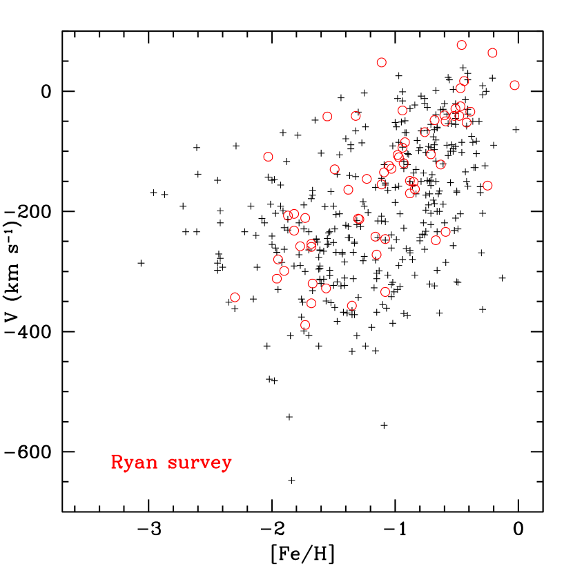
We have also included here results from preliminary spectroscopic binary orbital solutions from a second study of metal-poor stars, also selected on the basis of high proper motions. In 1992 we began radial velocity monitoring of 472 metal-poor stars selected from the sample of Ryan (1989; see also Ryan & Norris 1991a). Stars were selected if their estimated [Fe/H] values were or lower and the declinations were north of degrees. These data were obtained and analyzed in the same manner as reported by Carney et al. (1994): Metallicities were obtained from comparisons with a grid of synthetic spectra using a stellar effective temperature determined via photometry (see Carney et al. 1987; Laird et al. 1988a). Details of the second study will be presented later.
At the time of writing, we had obtained 28,564 velocities of 1,464 stars in the CLLA program, with a maximal span in the radial velocity coverage of almost 20 years. For the Ryan sample, we had obtained 3,812 velocities of 472 stars. Our goal for this second sample is much less ambitious since we have been interested primarily in measuring the stars’ metallicities, which requires only a few spectra (at most), and simply detecting shorter period binaries for follow-up observations. One goal, for example, was to refine the “transition period” that separates spectroscopic binary systems with circular orbits from those with eccentric orbits, which occurs at an orbital period of around twenty days. We also were searching for additional metal-poor double-lined systems that might show eclipses. While a few stars have radial velocity coverage of up to ten years, the average is much less, about two years, and in some cases the coverage is only a month or two. The Ryan sample is thus not yet a proper tool for detailed studies of binary statistics, but because the stars were selected in a very different manner than those in the CLLA survey, the Ryan sample provides a good check on the results from the CLLA survey.
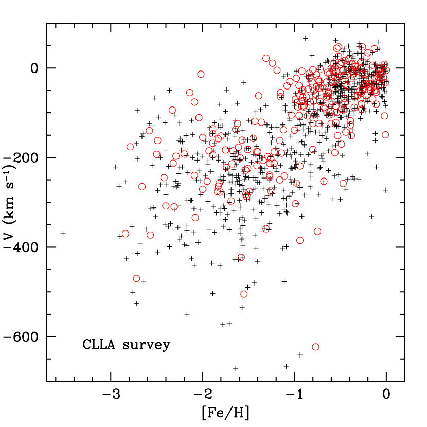
Within both surveys, all stars recognized as velocity variables (with final or preliminary orbital solutions, and those with secularly-changing velocities indicative of orbital motion) are identified here as “binaries”. To obtain a maximal identification of binaries for this paper, we also included visual binary stars and common proper motion pairs. To avoid overcounting, all of the latter, even when one or both of the members of the pair were themselves spectroscopic binaries, were counted as just one binary. Therefore, the G72-58 and G72-59 common proper motion pair, each of which has a published single-lined spectroscopic binary orbital solution, was counted as one binary at the relevant metallicity. In Figures 1a,b we show the distribution of Galactic V velocities of binary and single stars as a function of metallicity, [Fe/H], for [Fe/H] . (Please note that we have generally reported metallicities as “[m/H]” to indicate a mean metallicity rather than the abundance of a specific element. However, the calibrations have been done using [Fe/H], and to minimize confusion in comparisons with other studies, we refer here to all of our [m/H] results as [Fe/H].) Blue stragglers, subgiants, and all stars with significant uncertainties which compromised the determination of either metallicity or kinematics were rejected, leaving 756 single stars and 238 binaries in the CLLA program, and 349 single stars and 63 binaries in the Ryan program. The combined sample of 1406 stars has a binary fraction, , of %, where is defined as the number of binary stars divided by the total sample size. NOTE: we do not claim here that this is the “true binary fraction” of the high proper motion stars in our sample. Even with long-term radial velocity monitoring, very long period systems will be overlooked, as will systems with unfavorable orbital inclinations. No doubt common proper motion pairs remain to be discovered as well. Insofar as is determined without kinematic or metallicity bias, we can use to explore variations in binary fractions as functions of those parameters.
The calculation of stellar kinematics relies on relations between reddening-corrected color indices, metallicity, and absolute magnitudes, calibrated using stars in our surveys with good parallax data from the Hipparcos satellite. Details will be presented later, but we may estimate the approximate levels of precision in three ways. First, we have 16 common proper motion pairs of stars, for which we have determined the [Fe/H] values and the U, V, and W velocities independently. The average value of the velocity difference for the 48 separate velocity component comparisons is 8 km s-1, with only 12 having differences exceeding 10 km s-1, and only 5 with differences greater than 20 km s-1. Since identical proper motion values were employed, errors in the proper motions themselves must contribute additional uncertainties to our derived kinematics for individual stars. Assuming that the total proper motion error is less than 10%, and that it is apportioned equally among the three velocities, then to the 8 km s-1 uncertainty we should add to that roughly 10 km s-1 for stars with individual velocities typical of our program stars. Thus, independent of more “global” and systematic effects, including our derivations of [Fe/H] and , individual UVW velocities should be accurate to perhaps 15 km s-1. A more conservative choice would be 20 km s-1.
2 RESULTS
The key finding of this paper is revealed by a careful inspection of Figures 1a,b. They suggest that binaries may be less common for stars on retrograde Galactic orbits. Before discussing possible explanations for the phenomenon, we begin by exploring the binary fraction as a function of metallicity and other kinematical properties.
2.1 Binary Fraction as a Function of Metallicity
In these comparisons, and in all subsequent ones, we have analyzed the CLLA sample and the Ryan samples separately, and then the combined sample as well. The comparisons are done by first ranking each sample according to the variable being considered, metallicity in this case. Software divides the samples of single stars into a fixed number of bins (chosen to be 10 for the CLLA and combined samples, 5 for the Ryan sample). Bins differed in size slightly so that they would not overlap in the values of the parameters. Thus, no bin has any stars with the same [Fe/H] value as stars in any other bin. The binary star samples were then sorted according to these same metallicity ranges, enabling us to calculate the binary frequency, . We also computed the average span of the observations (in days) of the single stars within each bin to check that we had not introduced any bias due to greater or lesser time coverage as a function of metallicity, or any of the various velocity variables discussed below. (We do not include binary stars in the time coverage comparisons since observations of such systems were usually ended when the spectroscopic binary orbital solution was considered complete.) No such systematic variations in observing time coverage among the bins were apparent in any of the comparisons described in this paper.
Figure 2 shows the distribution of as a function of [Fe/H]. Note that the Ryan sample values tend to be lower than those of the CLLA survey. This is a consequence of the smaller number of radial velocity measurements per star and the smaller span in the observations. The bins in the CLLA sample have an average span of 3398 days ( days), while the bins in the Ryan sample have an average span of only 651 days ( days). There is a minor difference in as a function of metallicity, as seen in Table 1. For the combined sample % for [Fe/H] and % for [Fe/H] . If we consider only stars on prograde Galactic orbits (V km s-1), the modest difference in binary fraction between the metal-rich and metal-poor stars disappears, as summarized in Table 1. The combined sample has % for [Fe/H] and % for [Fe/H] . The conclusion to draw, at least to first order, is that among high proper motion stars, the binary fraction does not appear to depend strongly on metallicity. High velocity, metal-poor halo stars were able to produce binary systems as readily as low-velocity, metal-rich stars (see also Latham et al. 2002).
2.2 Binary Fraction of Stars on Retrograde Orbits
In Figure 3 we revisit the binary fraction as a function of metallicity, but divide the sample into two parts: prograde (filled circles) and retrograde (open circles). We have not distinguished between the halo or Ryan samples here: for clarity we show only the results for the combined sample. Two facts are prominent: (1) The retrograde portion is deficient in binaries relative to the stars moving on prograde orbits; and (2) Neither the prograde nor retrograde samples’ binary fractions depend on metallicity.
Figures 1a,b show that roughly half the stars with [Fe/H] are moving on retrograde orbits, while only 6% and 9% of the stars in the CLLA and combined samples with [Fe/H] have V km s-1. This low percentage is not, of course, surprising, since it simply means that for [Fe/H] , disk stars dominate the sample. To explore the differences between the prograde and retrograde stars more carefully, we show in Figure 4 the binary fractions as a function of the V velocity only for stars with [Fe/H] . The Figure shows clearly the deficiency of binary systems among stars moving on retrograde orbits. Table 1 quantifies these differences. The combined sample, with [Fe/H] shows a value for of % for stars on prograde orbits but only % for stars on retrograde orbits. This drops to only % for V km s-1. Figure 5 shows the cumulative single and binary star distributions of the combined sample as a function of V velocity, again for stars with [Fe/H] . A Kolmogorov-Smirnov test shows that we can reject the null hypothesis that both samples originate from the same parent population at the 99.998% confidence level. The impressions from Figures 1a,b are confirmed: The local sample of metal-poor high-velocity stars is deficient in binaries among stars on retrograde Galactic orbits.
2.3 Binary Fraction as Function of Other Velocities
Figures 6, 7, 8, and 9 show as a function of U, U, W, and W. Unlike Figure 4, there do not appear to be any significant trends in compared to these velocities, and simple divisions into low-velocity and high-velocity bins in Table 1 support this result. Kolmogorov-Smirnov tests of the distributions of these velocities show that the null hypothesis that, as a function of these velocities, the idea that the single and binary populations are drawn from the same parent populations cannot be rejected with reasonable levels of confidence. The only possible effect is seen in the W velocity. Indeed, for W +100 km s-1, Table 1 shows that has dropped significantly.
3 THE SEARCH FOR EXPLANATIONS
It appears, then, that there is a significant deficiency of binaries among metal-poor stars moving on retrograde Galactic orbits. What might cause this?
The explanations may be divided into two broad categories. The “simplest” class involves the destruction of binaries, creating the deficit we observe. This affects a significant fraction of the stars moving on retrograde orbits. Consider, for example, the 170 stars with V km s-1. The typical binary fraction in our sample of about 25% predicts that about 40 or more binaries should be found, while we detected only 17. For V km s-1, there are 374 stars, so over 90 binaries are expected, and only 47 are found. It appears that of order half of the binary systems on retrograde orbits would have to have been disrupted. That is about 10-15% of the total number of stars, so the effect is indeed significant.
The second broad class of explanations is that instead of binaries being disrupted, a mechanism exists to add significant numbers of single stars, thereby diluting the binary fraction. Consider again the same sample with V km s-1. Normally, 17 binaries would be found among a total population of only about 70 stars, not the 170 stars in our subsample. The dilution of the sample by “extra” single stars is thus very large: roughly 100 stars, or over 60% of the observed sample! For V km s-1, the 47 binaries should be found among a sample of 188 stars, not the much larger sample of 47 binaries and 327 single stars. In this case, there are 186 too many single stars. Both of these retrograde samples imply that of order 50% of the total samples would have to have been “added” as single stars.
Given the relative magnitude of the number of single stars to be added (% of the total sample) compared to the number of binary systems to be disrupted (%, but only about 10% of the total sample), it appears that the latter is a more plausible explanation than dilution by single stars. We therefore consider first whether binary disruption is a viable explanation.
4 DISRUPTION OF FIELD BINARY STARS WITHIN THE GALAXY
Binary systems may be disrupted by close encounters with compact or extended massive objects, and somehow the destruction mechanism must be enhanced for binary stars moving on retrograde Galactic orbits. We approach this topic from both theoretical and observational perspectives.
4.1 Theoretical considerations for tidal disruption
We ask if massive objects within the Galactic plane could be especially effective in disrupting those halo binaries that are primarily on retrograde orbits in the Galaxy. One differentiating characteristic for these stars is the larger relative velocity with which they encounter other objects in the disk. Although a larger relative velocity and shorter interaction timescale, such as between objects on prograde and retrograde orbits, generally implies a less destructive encounter, a larger relative velocity can drive encounters into the impulsive regime where collisions are most destructive. Binaries on prograde orbits would experience encounters at lower relative speeds, where the encounter may be adiabatic and the binary would be less vulnerable to disruption. The outcome of such encounters thus may depend on whether they are in the adiabatic or impulsive regimes.
A simple criterion for the impulsive regime is that the ratio of the encounter time to the binary orbital period , should be less than one (Spitzer 1958):
| (1) |
where we have taken the encounter time to be the interval that the stars take to cover a length equal to twice the collision impact parameter , at the relative velocity, . This condition means that, for the encounter to be impulsive, the impact parameter should be smaller than
| (2) |
An extreme case occurs if we take km s-1. The encounter would have to be within pc to be impulsive for a binary with an orbital period as long as years. This is a much longer period than those of the spectroscopic binaries that dominate the binary statistics in our study. Any shorter period binary would be in the adiabatic regime, where the energy transfer from the encounter to the binary becomes very inefficient. Since we see the binary deficiency among a sample of stars whose orbital periods are less than ten years, the relevant encounters must have been much closer, 0.002 pc, to enable impulsive encounters that would disrupt the binary systems.
Even encounters with massive objects, like giant molecular clouds, would affect only the widest binaries. Although the velocity kick produced by an impulsive encounter increases linearly with the mass of the perturbing object, from the impulsive condition, it is clear that an encounter with an extended object as large as a molecular cloud can not be close enough to be in the impulsive regime. The energy transfer in the impulsive regime quickly approaches zero as the physical size of the perturber increases, thus canceling the effect of the large perturber mass. Weinberg, Shapiro and Wasserman (1987) have investigated this phenomenon in detail and concluded that binaries with separations of 0.1 pc or less can survive for years when subjected to perturbations by stars and molecular clouds, if confined within the thin galactic disk, a condition unlikely to be met by the high-velocity retrograde stars in our sample. Thus tidal disruption due to encounters with stars and molecular clouds is not able to pack enough energy within the tight confines of the binaries in our sample to be able to explain the effect seen in Figure 4.
What about black holes? The binaries most readily disrupted are those with the lowest binding energies, meaning the widest separations. The widest known pairs in the solar neighborhood have projected separations of about 0.1 pc (Latham et al. 1984). Indeed, the widest pair in our samples, HD 134439 and HD 134440, has a projected separation of just under 0.05 pc. As Appendix A discusses, and Figure A-1 shows, binary separations this large imply large values of the impact parameter for massive point particle perturbers, and, therefore, only a modest density of perturbers is required. However, to disrupt the spectroscopic binaries in our sample, with periods of order a decade or less, and separations of a few AU, the impact parameter for encounters becomes extremely small, 0.001 pc or less, and the implied number density of perturbing black holes would be totally out of proportion compared to the inferred mass density in the Galactic plane (see Bahcall, Flynn, & Gould 1992).
4.2 Observational tests
We may also rule out lower velocity encounters with massive objects confined to the disk from a consideration of Figures 8 and 9. The stars in our sample with the W velocities closer to zero spend more of their time near the plane, and no binary deficiency is seen at such velocities.
The Galaxy’s central mass concentration has been claimed to be an effective environment for shredding star clusters (Aguilar, Hut, & Ostriker 1988). Could it also be efficient at destroying stellar binary systems? While the stars in our sample all lie within a few hundred parsecs of the Sun, in some cases the calculated perigalacticon distances are very small. This is strongly correlated with the Galactical orbital angular momentum, such that stars with V (and hence low angular momentum) fall towards the Galactic center. The commonly-adopted value for , the circular velocity at the Sun’s Galactocentric distance, is 220 km s-1 (Kerr & Lynden-Bell 1986), although there is some evidence for an even higher value of 270 km s-1 (Méndez et al. 2000). If the Galactic center plays a major role in binary disruption among our survey’s stars, we would expect to see a minimum in the binary frequency near V (or ) km s-1, with a much-reduced disruption effect and therefore higher binary frequency at both lower and higher V velocities (i.e., for stars with higher levels but opposite signs of angular momentum). Figure 4 is not consistent with this model. On the other hand, the V velocity is only a component of the total velocity in the solar neighborhood directed perpendicular to the direction toward the Galactic center. We therefore consider the combination of the V and W velocities. Figure 10 shows the binary percentages for the “VW” velocity,
| (3) |
Stars with very small values of VW pass close to the Galactic center, but the binary percentage remains constant, again indicating that the Galactic center is not responsible for tidally shredding most of the original binaries that have become single stars in our sample.
Finally, there is additional evidence that tidal disruption is not the primary explanation. We have shown that tidal effects are stronger for wider, less tightly bound, and longer-period systems, as discussed above. If tidal effects are the explanation of the binary deficiency seen in Figure 4, we expect that the surviving binaries would, on average, have shorter periods than for samples that have apparently not been subject to such disruptions. We therefore must look closely at the binaries at both ends of the V velocity distributions and compare the period distributions. We rely here only upon the CLLA sample since its time coverage is much longer and the numbers of observations have enabled us to obtain more spectroscopic binary orbital solutions than in the case of the Ryan sample. Specifically, we consider the three lowest and highest V velocity bins of our CLLA sample as shown in Figure 4, stars with V km s-1, and V km s-1, respectively, and to which we now refer as the retrograde and prograde binary samples. We consider first the systems whose periods are too long for us to determine: common proper motion pairs and visual binaries. Among the 9 binaries in the retrograde sample, three (%) fall into this long period regime. In comparson, 11 of the 46 binary stars in the prograde sample (%) fall into the long period domain. We note that one star in the retrograde sample and two stars in the prograde sample are both spectroscopic binaries as well as members of common proper motion pairs, but for the purposes of this part of our discussion, all we really wish to see if there is an absence of long-period systems among stars on retrograde vs. prograde orbits. We do not. We now consider the spectroscopic binary orbital periods (including preliminary periods) in the retrograde and prograde samples to see if the former show a dearth of long-period systems. Figure 11 shows the period distributions for the 7 retrograde and 35 prograde binaries for which we have determined or estimated periods. The distributions are very similar, and the Kolmogorov-Smirnov test shows that we cannot reject the hypothesis that they are drawn from the same populations.
We conclude that in our binary-poor retrograde sample there does not appear to be any preference for short-period “survivors” vs. long-period binaries predicted by tidal-driven disruption mechanisms.
No binary disruption mechanism appears to be capable of explaining the paucity of binaries moving on retrograde Galactic orbits, and we are forced to explore possible sources of excess numbers of single stars even though, as we have seen, we will need to identify a source or sources of single stars for almost 50% of the stars moving on retrograde Galactic orbits.
5 GLOBULAR CLUSTERS AS SOURCES OF SINGLE STARS
We explore here the two options that rely on globular clusters and which could provide single stars while sequestering binary systems. In the first case we assume that a binary-single star encounter within the cluster leads to a more tightly bound binary system and the ejection of a single star. In the second, we assume that dissolved (or dissolving) clusters have primarily populated their outer regions with single stars, thereby increasing their numbers in the field, and decreasing the binary fraction, at least in restricted regions of velocity space.
5.1 Ejection of single stars
To explain Figure 4 by binary disruption within Galactic globular clusters would require that the stars on the most extreme retrograde Galactic orbits acquired a “velocity kick” during a binary disruption. The average metal-poor halo star or cluster has a mean V velocity of km/s, and the one-dimensional velocity dispersion of the field stars and the ensemble of metal-poor globular clusters is of order 100 km s-1. To introduce the sort of asymmetry seen in Figure 4 therefore requires that the kick should add about the magnitude of the halo’s velocity dispersion to the stars’ space motions. Qualitatively, the idea has some merit, at least for the V velocity. Single stars ejected toward more negative V velocities would provide an excess of single stars, which we will have interpreted as a deficiency of binaries. Because stars ejected toward more positive V velocities will have space velocities closer to the Local Standard of Rest, they would be less likely to appear in samples, like ours, that are selected from proper motion catalogs.
Quantitatively, this explanation has problems. First, the original binary periods would have been on the order of days ( and km/s leads to P days, with P). It is unlikely that there were enough such short-period halo binaries available for disruption. More important, however, the ejection should occur over 4 steradians, and so it should be manifested in the U and W velocity directions as well. Figures 6-9 rule out this explanation.
5.2 Globular cluster dissolution?
Here we ask if the low fraction of binary systems on retrograde orbits might have been caused by the evaporation of stars from a globular cluster or clusters moving on retrograde orbit(s). Dynamical evolution of a globular cluster, for example, leads to a greater central concentration of tight binary systems and a more extended distribution of lighter single stars (see Hut et al. 1992 for an excellent discussion). Many of the original globular clusters in our Galaxy may have undergone such evolution, to the point of much reduced sizes or total evaporation (Aguilar 1993). There are several lines of evidence that support the idea that many of the Galaxy’s original clusters have suffered such a fate. First, Chernoff & Djorgovski (1989) found that clusters within the central 3 kpc of the Galaxy are more concentrated and more likely to show central power-law density profiles, indicative of post-core collapse evolution, and in agreement with the cluster evolution models of Chernoff, Kochanek, & Shapiro (1986). Second, the selective erosion of clusters in radially plunging Galactic orbits can explain the observed difference in kinematics between the stellar halo and globular clusters (Aguilar, Hut, & Ostriker 1988). Third, studies of young stellar systems with masses like those of globular clusters in starburst galaxies and merging galaxies have revealed that the mass spectrum follows a power law (see Whitmore 2003 for a review; also Whitmore et al. 1999; Zhang & Fall 1999). This is completely unlike that of the current Galactic globular clusters, which has a Gaussian-like mass distribution (Harris 1991). One way to evolve from a power law distribution to that observed today is through more rapid dissolution of lower mass systems (see Fall & Zhang 2001; Vesperini & Zepf 2003). Finally, we can actually see cluster dissolution happening through detection of cluster tidal tails (Meylan & Heggie 1997; Leon, Meylan, & Combes 2000; Odenkirchen et al. 2001, 2003; Siegel et al. 2001). We recognize the difficulty, however, of relying on the dissolution of many clusters to provide the excess of single stars, because this mechanism then also requires a means to favor dissolution of clusters moving on retrograde rather than prograde orbits.
We approach this issue from two perspectives, asking first if there is a difference in terms of dynamical evolutionary state for clusters moving on prograde or retrograde orbits, and then seeking signs for dissolved clusters in the form of “moving streams” in velocity space. Detection of such streams would have relevance to the search for dark matter substructure within the Galactic halo (Ibata et al. 2002) since significant departures from a smooth mass distribution (i.e., substructure) enhances dissolution of streams, their detection may provide a limit to the degree of the substructure in the Galactic halo.
We have used the same database as Chernoff & Djorgovski (1989) to evaluate the dynamical evolutionary state of globular clusters. The two relevant parameters are the concentration class, , and the type of model applicable to the stellar distributions. Specifically, which clusters show evidence for post-core collapse? Because Chernoff & Djorgovski (1989) found clear evidence favoring enhanced dynamical evolution for clusters closer to the Galactic center, we limit our study to those clusters which are not only outside some limiting Galactocentric distance, but also restrict our study to only those clusters whose Galactic orbits do not carry them closer than a certain distance, using the orbits calculated by Dinescu, Girard, and van Altena (1999). For the 19 clusters (excluding the very distant cluster Palomar 3) with perigalacticon values exceeding 3 kpc, five are classified as “PCC” or “PCC?”, and four of those are on prograde orbits. The mean concentration class of the nine clusters on prograde orbits is (), while that of the four clusters on retrograde orbits is (). If we move the perigalacticon limit out to a distance of 5 kpc, there is only one “PCC” cluster, NGC 7078 (M15), and it is moving on a prograde orbit. The same four clusters define the retrograde sample, but the prograde sample has declined from nine to five clusters, and (). There is certainly no evidence for enhanced dynamical evolution of globular clusters moving on retrograde orbits. Indeed, if anything, the evidence favors enhanced evolution for clusters moving on prograde orbits.
We turn now to the search for star streams. No globular clusters are close enough themselves for their stars to be seen in our survey, but moving streams occupy larger volumes than do individual clusters, and while the space densities of stars in streams are low, their densities within velocity space may lead to their detection, even in our modest sample. Because the physical volume of our survey is small, detection of stars in a stream requires that each star have very similar space velocities. Thus the U, V, and W velocities should be quite similar, consistent basically only with observational uncertainties. With the exception of Cen, stars in any one globular cluster have very small (e.g., Langer et al. 1998) to non-measurable differences in [Fe/H] (Suntzeff 1993). We therefore expect any candidate stream to involve stars with very similar metallicities if it originated from a dissolved or dissolving globular cluster. We therefore conduct a search for dissolved clusters by confining searches to narrow windows of metallicity as well as of velocities.
How many streams might we expect? Our full sample of stars with reliable metallicities includes 1638 stars, with an average distance of 162 pc, and 90% of them lying within 330 pc. The metal-poor, high-velocity stars may be seen to greater distances due to their higher tangential velocities. The 423 stars with [Fe/H] and V km s-1 have an average distance of 286 pc, and 90% of them lie within 470 pc, a significantly larger volume. For V km s-1, the average distance increases to 325 pc, and the 90% distance increases to 520 pc. Our maximal sample volume is thus about pc3 (and is much smaller for slower-moving objects). The two nearest globular clusters are M4 and NGC 6397, with distances of about 2 kpc, and have proper motions of about 0.02″ per year (Dinescu et al. 1999), corresponding to tangential velocities of about 200 km s-1. For these clusters’ stars to have proper motions large enough to have been detectable in our sample, with a proper motion limit of ″ per year, the clusters’ stars would have to be ten times closer, or about 200 pc. There are too few clusters in the Galaxy now for us to have one so nearby. But if most of the Galactic halo’s field stars came from globular clusters, then since the halo field stars’ combined mass exceeds that in the current population of globular clusters by a factor of about one hundred, there may have been of order a hundred times as many clusters as now exist (or more, given dissolved clusters’ lower masses). Therefore the typical distance from the Sun may have been (100) smaller than it is now, and the nearest cluster would have been only 400 pc away, and thus we might expect to see evidence for its remnants in the form of a star stream.
However, dissolved clusters occupy much larger volumes than bound clusters, and so would be even nearer to the Sun, on average. And, as we noted above, while the spatial densities of stars might be low, they might be discernable in velocity space. A factor of roughly one hundred increase in spatial number density of dissolved clusters means that the proximity of a stream to the Sun is increased by another factor of (100), and hence there may well be several to many streams from dissolved or dissolving clusters in the solar neighborhood. How many there are depends on how uniformly the stars are dispersed along the clusters’ orbits and, of course, how many clusters originally were formed in the Galactic halo. If most of these “dissolved” clusters actually take the form of lighter single stars dispersed along the orbit plus an undetectable remnant of tightly packed binary stars and binary stellar remnants, we might be able to explain our observation of a deficiency of binary stars on retrograde orbits. We would, of course, still have to explain why dissolved clusters should be found preferentially on retrograde orbits. Or we could invoke a single cluster, whose binary-rich remnant is beyond our view, and whose single stars populate a significant fraction of the metal-poor stars in the solar neighborhood.
How many stars from an individual cluster might we expect, assuming its orbital stream passes through the local volume? Let’s assume that the cluster stream’s stars have diffused uniformly along the orbit, but perpendicular to the stream by an amount considerably smaller than the diameter of our local sampling volume. In that case the number of detectable stars would be related to the number in the original cluster, , and the ratio of the length of the orbit within the local volume divided by the total orbital length. Assuming a circular orbit, the number of detectable stars would be
| (4) |
where is the thickness of the sample volume and is the distance of the Sun from the Galactic center, 8.0 kpc. Thus for = and = 300 pc, we might find as many as a thousand stars, with longer orbits leading to fewer stars in our search volume. And notice that the odds are somewhat improved for stars on retrograde orbits since the effective local sample volume increases in size.
Our actual net, however, would be far less than a thousand stars, for two reasons. First, the least massive globular clusters would have dissolved most rapidly, and the original cluster might have included only stars rather than . Second, our surveys cover only a limited range of temperature or color, and hence a limited range of absolute magnitude. Hence the surveys cover only a small fraction of any cluster’s stars. Consider the luminosity function of the globular cluster M13 (Richer & Fahlman 1986) shown in Table 2. If we consider only those stars in our surveys with metallicites between [Fe/H] = and (compared to that of M13, with [Fe/H] = ), we find a total of 2, 94, 87, and 42 stars in the color ranges that correspond to the absolute and apparent magnitudes of the M13 luminosity function. Notice that our survey luminosity function is dropping at redder colors (and fainter absolute magnitudes) than is the M13 luminosity function. In the final column of Table 2 we assume that the color range corresponding to ()0 = 0.414 to 0.531 is complete in our surveys. We normalize the other magnitude and color bins by the ratio of 43.3/94 times the number of stars in our surveys. The total number of stars in our survey is then 103.6, compared to the 973.6 in M13. In other words, the color and magnitude selection criteria in our surveys mean that our sample is likely to include, at most, only 10% of any dissolved cluster’s main sequence stars. This is of course an upper limit since it is unlikely that our surveys would find all of a dissolved cluster’s stars in our search volume in the ()0 = 0.414 to 0.531 magnitude range. And the M13 luminosity function is itself incomplete at the faintest end. We conclude that a completely dissolved globular cluster whose orbital stream passes near the Sun and whose stars are moving at high velocities relative to the Sun might yield only a few stars.
If dissolved or dissolving clusters is the explanation for the retrograde binary deficiency, we have several new questions to answer. First, do we see any signs of streams? While streams may be disrupted, their detection would lend support to this hypothesis. Second, if they are detected, are they moving primarily on retrograde orbits? If multiple dissolved clusters are the cause of the effect, we then also require an enhancement effect to preferentially populate clusters moving on retrograde Galactic orbits. On the other hand, if only a single large object which had a retrograde orbit is involved, are there other clues that might distinguish, for example, an accreted dwarf galaxy from dissolved Galactic globular clusters?
6 SEARCHING FOR STREAMS IN THE HALO
6.1 Historical Background
There is a long history of searching for moving groups of stars, also called star streams, in local samples of stars. Eggen’s (1958a,b,c; 1960a,b,c,d) work on the Hyades, Sirius, and many other possible moving groups stands out in particular, as well as his work on seeking moving pairs of halo dwarfs with RR Lyraes to calibrate the luminosities of both (Eggen & Sandage 1959; Eggen 1977). His work followed the “convergent point method” for the estimation of the distance to the Hyades. The essence of the method is that the angle between the cluster’s location and its measured convergent point provides a relation between the radial and tangential velocities of the cluster. Since radial velocities and proper motions are measurable, the measurement of the angle leads to the relation between tangential velocity and proper motion, meaning the distance. Eggen employed this technique in assuming an association between two or more stars, determining a convergent point, deriving distances to the individual stars, and then testing the association by seeing if a plausible color-magnitude diagream was the consequence. He did not, however, test for consistency of metallicities, largely because they were not well-determined at the time of his work.
Two other more recent methods assume the distances are relatively well determined, and seek slightly different means to identify kinematical relationships that point to shared dynamical histories. This is not a simple task, for two reasons. First, stars may be relatively dispersed, even along a common “orbit”. To counter this, recourse is often made to “conserved quantities” that may link stars or even clusters travelling in somewhat different parts of the Galaxy’s gravitational potential. Second, these conserved quantities are few since the Galaxy’s gravitational potential is not point-like, and is not even very well understood.
The first method, which we have employed, has been used to study stars within a few hundred parsecs of the Sun. Carney et al. (1996) assumed that the planar angular momentum, , should be a relatively well-conserved quantity, and in the solar neighborhood it follows directly from the Galactic V velocity. Total orbital energy should also be relatively well conserved, and this may be derived from the “rest frame velocity”, :
| (5) |
Carney et al. (1996) suggested that structure in the V- plane suggested that outer halo stars, now in the solar neighborhood, may have been accreted from small galaxies. But a search for clumping of stars in the V- plane did not reveal any “obvious” co-moving stars that might not have arisen by chance. By “obvious”, we mean a purely subjective assessment of the appearance of the diagram, and “apparent” groupings of stars.
Helmi et al. (1999) employed a somewhat similar method but replaced the orbital energy with another form of angular momentum, , whose axis is orthogonal to the disk’s axis of rotation. They found a very intriguing clumping of stars. Not all stars in the clump may be affiliated, however, since the signs of their angular momenta differ, but the results remain intriguing.
Both the above methods, and indeed any method devised to search for moving groups, are vulnerable to the vagaries of chance. How confident can we be that a clustering or clumping of stars in some two-dimensional, or even three-dimensional, location is pointing to members of a dissolved cluster or to just a random grouping? We re-investigate this problem here.
6.2 Searching for Streams: Our Approach
6.2.1 Preliminary identification of streams
As discussed above, our sample of stars is confined to within a few hundred parsecs of the Sun. We do not need to rely on only two possibly conserved quantities, but we may use the full three dimensional information contained in the U, V, and W velocities. For a stream to maintain coherence over a period equivalent to several Galactic orbits, stars still belonging to a stream should differ by no more than a few kilometers per second in any of these three velocities. This defines our basic approach. We searched through the entire sample, looking for groups of stars that lie within a cube of of, say, 40 km s-1 on each side in velocity space. If a group has four or more stars, we then derive the velocity dispersion, (), for all three velocities, requiring that each be smaller than some small, adopted value. Once such a group is identified, all of its members are removed from the sample to avoid assigning stars to multiple groups before the search is continued. It should be noted that the search algorithm is not unique. Searching our sample in a different order will find the same general groups, but perhaps with a slightly different mix of identified members.
6.2.2 Monte Carlo experiments
We must now test the significance of the possible moving groups found in the observed sample by comparisons with results with those found in simulated surveys of a model sample with similar kinematics as ours, but which lacks any moving groups.
We take this model sample to consist of a sphere extending 500 pc in all directions from the observer, and with a constant star density, an assumption that is quite reasonable for the metal-poor halo population we’re considering. The model employs = 220 km s-1, and the velocity ellipsoid for the halo derived by Sommer-Larsen (1999), with km s-1, km s-1, and km s-1. We adopt a lower limit to proper motions of 0.27″ per year, typical of the Lowell Catalog which is the primary source of our program stars. The distance limit is actually irrelevant for the modelling because the proper motion constraint leads to unrealistic tangential velocities for most stars at distances of only about 300 pc. For the same reason, the magnitude limits of the Lowell and NLTT catalogs do not affect the results of our modelling.
We searched for kinematical groups using the same criteria discussed above for , (), and . We explored a range of different values of (), from 40 km s-1 down to 25 km s-1. Each Monte Carlo simulation was obtained from an ensemble of simulated surveys. Table 3 compares the results from our real sample of 692 stars with [Fe/H] to those of the Monte Carlo experiments. As expected, the number of possible groups identified in the modelling rises as the () criterion is relaxed to larger values. So does the number in the real sample. Figure 12 compares the two sets of results graphically. We conclude that there is no compelling evidence for moving groups in our sample of local metal-poor stars using only the three velocities as the basis for the search.
The above result shows that we have failed to find evidence for any major star stream or signs of numerous smaller star streams with relatively small velocity dispersionss that have an arbitrary range of metallicities, as might be expected from accreted galaxies.
This leads, of course, to the next question: Is there evidence for dissolved globular clusters? Here we now must include metallicity as a search criterion, because with the exception of Cen, stars in any one globular cluster have very small (e.g., Langer et al. 1998) to non-measurable differences in [Fe/H] (Suntzeff 1993). We therefore expect any candidate stream to involve stars with very similar metallicities if it originated from a dissolved or dissolving globular cluster.
As before, the modelling requires a good representation of the distribution of the values of the variable, metallicity in this case. We have adopted the measured metallicities of our program stars, and smoothed the distribution to provide our adopted model distribution, as shown in Figure 13. The modelling was repeated, following exactly that for the kinematical searches described above, but with the addition of [Fe/H] as a variable. We varied the allowable range in the metallicity spread, [Fe/H], from 0.05 up to 0.60 dex. (Please note that our measured relative metallicities should be good to 0.1 dex.) Table 4 compares the results of the searches through the real sample and the Monte Carlo simulations as a function of and [Fe/H] for groups with 4 or more members.
As we relax the velocity and metallicity constraints, Table 4 shows that the number of identified moving groups in the observed sample increases, but so does the number in the simulated surveys. Within the small number statistics, both numbers are in fact quite similar, suggesting that none of the identified groups are significant. There is one possible exception. In looking in the column for [Fe/H] 0.20, one group in the observed sample remains, while the probability of finding such a group with km s-1 has declined to 30%. The possible stream consists of five stars, whose properties are summarized in Table 5. The group’s members have little planar orbital angular momentum, and we have estimated their peri-Galacticon distances to lie only about 0.4 kpc from the Galactic center. Their putative parent cluster is therefore a likely candidate for tidal disruption during a close passage to the Galactic center. The apo-Galacticon distance is only about 9.6 kpc, so the cluster is unlikely to have been accreted from another galaxy.
Even if this stream does represent a dissolved globular cluster, it falls very far short of explaining the binary deficiency seen among stars moving on retrograde Galactic orbits. First, while we have noted already that tidal disruption of clusters passing near the Galactic center could cause an effect, it would not produce the binary deficiency seen in Figure 4. Second, the magnitude of the effect is far too small. We have seen that to explain the binary deficiency for stars with [Fe/H] and V km s-1 requires the addition of well over one hundred single stars. Five single stars is inadequate by a factor of at least twenty. We conclude that while there may be one moving group in our sample of stars, dissolved globular clusters are unlikely to have provided a surfeit of single stars, and hence the apparent deficiency of binary stars, on retrograde orbits.
7 SINGLE STARS FROM ACCRETED GALAXIES?
Globular clusters evolve dynamically, eventually populating their outer regions with lighter single stars, and shedding them as the evolution continues. But dwarf galaxies are hardly ideal places to seek such segregation of single and binary stars. The relaxation timescale is given by
| (6) |
where is the number density of stars, is the rms stellar velocity, ln = 0.4 N, N is the total number of stars in the system, and N = (Spitzer 1987). Relaxation timescales are essentially two-body processes, and the low stellar densities in the Galaxy’s current complement of satellite galaxies appears to make dynamical relaxation timescales far too long for the current (surviving) dwarf galaxies to have evolved quickly enough so that single stars would be shed much more readily than heavier binary stars. There are a couple of reasons, however, to not dismiss the idea too hastily. For one, Hurley-Keller, Mateo, and Grebel (1999) found evidence for a central concentration of photometric binaries in the Sculptor dwarf galaxy. Thus even though we may not understand the single star vs. binary star segregation in that dwarf galaxy, the segregation may exist nonetheless.
We can speculate a bit about how mergers might occur, following the discussion of Walker, Mihos, & Hernquist (1996). Their work focussed on a merger involving a dwarf galaxy on a prograde orbit on a modest inclination to the Galactic plane. The orbital evolution and tidal dismemberment of a victim is relatively rapid, with the consequence that the galaxy’s orbit becomes nearly co-planar and the merger is largely complete in a timescale of order 1 Gyr. They did note, however, that the evolution is much slower for a merger involving a dwarf galaxy on a retrograde orbit. Thus a dwarf galaxy on a retrograde orbit has a longer time in which to evolve, both dynamically and chemically. Walker et al. (1996) did not study this case in as much detail, but the more specific case of the massive globular cluster Centauri has been studied by Tsuchiya, Dinescu, & Korchagin (2003) and Tsuchiya, Korchagin, & Dinescu (2004). This is relevant here because Cen has been suggested (Freeman 1993) to be the former nucleus of a captured satellite galaxy, and its current Galactic orbit is planar (W = km s-1) and retrograde ( km s-1; Dinesci, Girard, & Van Altena 1999). Mizutani, Chiba, & Sakamoto (2003) suggested that the stellar debris from such a remnant would have retrograde motion of V km s-1. Unfortunately, no one has included mass segregation and other dynamical effects in the evolution of the victim galaxy as yet. However, there is chemical evidence that supports the idea that Cen may have had a fairly long time to evolve dynamically. Based on the enhancement of -process elemental abundances, Norris & Da Costa (1995), Smith et al. (2000), and Rey et al. (2004) have suggested a chemical enrichment history stretching over 2 to 4 Gyrs, which is consistent with the orbital evolution timescale of Tsuchiya et al. (2003, 2004).
More recently, Meza et al. (2004; hereafter M2004) have computed a detailed model involving the dissolution of a small galaxy () that leads to a significantly increased number of stars in the Galactic halo and a remnant moving on an orbit comparable to that of Cen. As in the above simulations, the stars absorbed by the Galaxy are distributed rather widely in phase space. Nonetheless, M2004 noted that there is an excess of stars in the solar neighborhood with planar angular momenta comparable to that of Cen. We are thus encouraged to seek an explanation for the deficiency of binary stars on retrograde Galactic orbits by seeking a possible connection with Cen.
If this idea has merit, and our apparent deficiency of binary stars on retrograde orbits is in fact caused by an excess of single stars shed by a dwarf galaxy, why did it elude our detection in the search for streams? The answer lies in the resultant velocity dispersion of the remnant’s stars in the solar neighborhood: it may be too large for us to have detected it readily, as the models of M2004 suggest.
7.1 The Chemical Footprint of Centauri
Are there other ways to detect such a system? Possibly, and here we explore the idea that a significant fraction of the single stars moving on retrograde orbits may be related to the putative satellite galaxy of which Cen was the nucleus. We pursue this idea partly because of the dynamical clues mentioned above, but also because the discussion will serve as an illustrative attempt as to how to seek common origins, using abundances as well as dynamics, since Cen may not, in fact, represent the only evidence for a dissolved dwarf galaxy moving on a retrograde Galactic orbit.
There are three separate questions to be explored. (1) Do the field stars have a similar mean metallicity as the former galaxy, represented here by the globular cluster? In the absence of knowledge about a possible relation to a surviving cluster such as Cen, we can ask if the mean metallicity of the single stars on retrograde orbits differs significantly from the binary stars on retrograde orbits (presumably not contributed primarily by the accreted galaxy) and the metal-poor single plus binary stars on prograde orbits. (2) Are there any significant differences in the detailed chemistry of these samples that might suggest a chemical relationship with Cen? In other words, do the retrograde single stars differ in [X/Fe] patterns from the other field stars and, in this case, are they similar to the stars in Cen? This latter test is not definitive, since stars in the outer regions of a dissolving galaxy may not have shared the same chemical evolution as stars in the central regions represented, perhaps, by Cen. (3) If mass segregation has occured in the merging galaxy such that it shed single stars most readily, is the central remnant, Cen, unusually rich in binary stars? We explore these three questions in turn.
7.1.1 Metallicity distribution
As we discussed in Section 6.2 and the introduction to this section, a dissolved galaxy may shed stars with a wide range of metallicities, complicating their identification in the field population. There are two fundamental questions to be addressed. The simplest one is to see if the prograde and retrograde single and binary stars show similarities or differences with the mean metallicity of Cen. We must recognize here that the cluster may not be representative of the former galaxy’s true mean metallicity or metallicity distribution.
We begin by defining a reference sample involving stars moving on prograde Galactic orbits. We have not found a significant difference in the metallicity distributions of the single and binary stars with [Fe/H] and moving on prograde Galactic orbits ( V km s-1), so we merge those samples, totaling 223 stars. In Figure 14 we show the histograms of both single and binary stars with [Fe/H] and V km s-1. We chose this domain on the basis of Figure 4. We show similar results, but for V km s-1, in Figure 15. We chose this value based on the velocities of field stars from the dissolved parent galaxy of Cen (Mizutani et al. 2003), and because this velocity regime shows an even greater deficiency of binary stars (Table 1).
The mean metallicity of Cen is about , but, unfortunately, that is also the peak of the metallicity distribution of the Galactic halo (consider the prograde sample; see also Laird et al. 1988b; Ryan & Norris 1991b). Figures 14 and 15 show peaks in the metallicity distributions for all the samples, so this comparison offers us no compelling evidence for a relationship with Cen. We must also expect that the stars accreted from a dissolving dwarf galaxy will have a range in metallicity, and, as has been known for a long time, so do the stars of the cluster, from [Fe/H] to .
Instead of comparing the mean metallicities of field stars to that of the cluster, we turn, instead, to testing the predictions of our model. Specifically, do the single stars moving on retrograde orbits, which may have arisen in significant part from the hypothesized dissolving galaxy, differ in their metallicity distribution from binary stars moving on retrograde orbits, or from the single plus binary stars moving on prograde Galactic orbits? We note that such comparisons may not be critical tests, simply because the Galactic halo and the accreted galaxy may well have similar metallicity spreads, which would be expected if both evolved as “closed box” systems. We define the prograde sample to be those stars with [Fe/H] and with V km s-1. Using the Kolmogorov-Smirnov test, we find that we can reject the hypothesis that stars in this metallicity range and with km s-1 were drawn from the same parent population as the prograde sample with a confidence level of only 38%. For km s-1, the confidence level is 78%, but this remains unconvincing. The confidence levels in comparing the single stars and binary stars with km s-1 and km s-1 are not compelling either, being only 77% and 48%, respectively, although the sample sizes are very small due to the limited number of binaries moving on retrograde Galactic orbits (47 and 17 stars, respectively). The K-S tests do not, therefore, provide any evidence in support of our hypothesis that a significant fraction of the single stars moving on retrograde Galactic orbits originated in the dissolved and accreted dwarf galaxy. (But the test only makes sense if the metallicity spread of the galaxy and the Galactic halo are significantly different.)
There is one interesting comparison. The prograde and retrograde binary samples do appear to differ in their metallicity distributions: the confidence levels for the km s-1 and km s-1 samples are 90% and 88%, respectively. We have no explanation for this effect.
We are therefore compelled to look more carefully for characteristics that might distinguish Cen from the normal field stars.
7.1.2 Abundance Patterns
The chemical enrichment history of Cen is rather different than that of other globular clusters, as well as the field halo stars, which is one reason why it has been suggested to be the remnant nucleus from a satellite galaxy. Specifically, not only do its stars show a wide range in iron abundances, but, except for the most metal-poor stars in the cluster, its members show strong signs of enhancement of -process nucleosynthesis. Norris & Da Costa (1995) discussed this characteristic at length, and their Figure 13 summarizes the situation well. The “light” -process element Y is enhanced in the Cen stars, relative to other globular clusters, and presumably single field halo stars, by about 0.3 dex or so over the range [Fe/H] . The “heavy” -process element Ba is similarly enhanced over the same range in [Fe/H]. At lower metallicities, the stars in Cen more closely resemble other clusters and field stars in [Y/Fe] and [Ba/Fe], so we restrict our comparisons between retrograde and prograde field stars to this limited intermediate metallicity regime, [Fe/H] , to maximize the differences between normal field stars and the giants in Cen and still avoid trends in [Y/Fe] and [Ba/Fe] with [Fe/H].
Do the single stars moving on retrograde Galactic orbits divide into normal and abnormally high [Y/Fe] or [Ba/Fe] abundance ratios? We first re-explore the expected abundances of Y and Ba among halo stars. The observational situation is well reviewed by McWilliam (1997; and references therein), and updated by Burris et al. (2000). To minimize any possible systematic effects, such as might exist, for example, between analyses of dwarf and giant stars, we explore only the published abundance analyses of stars in our studies of stars with large proper motions. To further minimize systematic effects, we employ only two relatively large studies of the chemical abundances of field stars, those of Fulbright (2000; hereafter F2000) and Stephens & Boesgaard (2002; hereafter SB2002). Figures 16 and 17 show the trends of [Y/Fe] and [Ba/Fe] for single and binary stars with [Fe/H] moving on prograde orbits. While there is a strong decline seen in [Ba/Fe] for [Fe/H] , we are concerned only with [Fe/H] , since that is the regime in which Cen differs most strongly from other clusters and from field stars. We see that over this metallicity range, the prograde sample has approximately constant values of [Y/Fe] and [Ba/Fe].
In Figures 18 and 19 we now consider [Y/Fe] and [Ba/Fe] vs. the V velocity. Figure 18 hints that stars on strongly retrograde orbits, V km s-1, may consist of two groups, one with elevated [Y/Fe] values and one with slightly lower values of [Y/Fe]. We have provided the basic data for these 8 single stars (and the one binary system) in Table 6. For the 8 single stars with V km s-1, the mean value of [Y/Fe] is (), and the mean value of [Ba/Fe] is (). While the mean [Y/Fe] value for the 8 single stars with V km s-1 is similar to the prograde sample, , the rms spread is not: dex. At the risk of over-taxing a small sample, we divide these 8 stars with V km s-1 further, into “Sample A” with [Y/Fe] 0, and “Sample B”, with [Y/Fe] 0. For A, [Y/Fe] = (), while for B, [Y/Fe] = (). The spreads are more consistent with those obtained for the prograde sample, but the separation in [Y/Fe] is large, dex. This is the same magnitude that distinguishes the giants in Cen from those in other globular clusters! Of course, dividing a sample into high and low regions must result in a net difference between the two groups, but let us proceed nonetheless. Further challenging small number statistics again, it is noteworthy that the numbers of stars in Samples A and B are comparable, about what is needed if the low binary fraction arises from an influx of single stars into the retrograde sample (of order 50%, according to the discussion in Section 3). Qualitatively, the [Y/Fe] results agree with the idea that the excess of single stars could have arisen from the dissolution of the parent galaxy of Cen, if it somehow had segregated single and binary stars. However, we note that K-S tests of the [Y/Fe] patterns for single stars on prograde and retrograde orbits do not confirm any significant difference, due to the small sample sizes or the lack of a real difference.
What about [Ba/Fe]? Figure 19 does not reveal as dramatic a separation in [Ba/Fe] values for stars moving on retrograde Galactic orbits. Further, the results of Norris & Da Costa (1995) suggest that the difference should be even more striking for [Ba/Fe] than for [Y/Fe]. The K-S probabilities again do not demonstrate any significant difference between the single stars moving on prograde and retrograde orbits. But there is, nonetheless a hint that differences may exist. The 8 single stars with V km s-1 have a mean [Ba/Fe] abundance ratio of (). The 8 single stars with V km s-1 have a marginally lower value, ( = 0.13) dex. However, it is very interesting that we find the same four stars that define Sample A ([Y/Fe] 0) have [Ba/Fe] = (), while for Sample B, [Ba/Fe] = (). The difference in [Ba/Fe] between Samples A and B appears to be real, formally dex, but the magnitude falls short of what we expect, dex, based on the results of Norris & Da Costa (1995).
We conclude that the [Y/Fe] and [Ba/Fe] values hint at a bimodal distribution in the -process abundances for stars moving on retrograde Galactic orbits. However, the numbers of stars studied remains small, and therefore there is not yet compelling chemical evidence that the single stars moving on retrograde orbits originated from the dissolved parent galaxy of Cen or any other different source. Larger sample sizes may prove useful in confirming the possible differences in [Y/Fe], and perhaps [Ba/Fe] as well. It would also be interesting to explore the [Y/Fe], [Ba/Fe], and other -process abundances with -process abundances such as Eu, in more detail. (F2000 reported Eu abundances for only two of the single stars with retrograde orbits, and SB2002 did not report any Eu abundances.)
M2004 have also raised the idea that field stars that once belonged to the parent galaxy of Cen may have a distinctive pattern of the abundances of the “” elements, taken here to be Mg, Si, Ca, and Ti. M2004 employed the compilation of abundance analyses from Gratton et al. (2003), and noted that the distribution in the planar angular momenta shows a peak at about the value expected for stars that could be related to Cen or its now-dissolved parent galaxy (Dinescu et al. 1999). Since the Galactic orbit of Cen is now close to the Galactic plane, M2004 winnowed the Gratton et al. (2003) sample further to include only stars with moderately retrograde or very weakly prograde Galactic orbits, and with W velocities (W 65 km s-1) such that the stars do not stray far from the plane. They found that these kinematic selection criteria led to stars that did not show the characteristic peak near 0 km s-1 in the distribution of U velocities, and they seized on this to help distinguish a sample of 11 field stars (with U 50 km s-1) that might be related to Cen. Those stars are indeed interesting because, like the other field stars, they show elevated values of [/Fe] ( for low metallcities, and declining [/Fe] values for higher [Fe/H]). Unlike the bulk of the field stars, however, M2004 found that this sample appears to begin the decline in [/Fe] at [Fe/H] , rather than at more typical of field halo stars. This “earlier” decline may signal by a slower rate of star formation, which, as we have discussed above, appears to be a hallmark of the chemical evolution of Cen.
However, we do not believe that these stars are, in fact, necessarily related to Cen. The primary argument against the relationship is that Norris & Da Costa (1995) did not find reduced values for any of the “” elemental abundances for cluster stars with [Fe/H] . We are also concerned by the kinematical selection criteria employed by M2004. By considering stars with, effectively, very low V and W velocities, stars with low U velocities will be selected against in proper motion samples (which help define the stars analyzed by Gratton et al. 2003) and do not commonly exist in this radial region of the Galaxy, where orbital energies are typically 200 km s-1. In other words, the kinematic criteria employed by M2004 would naturally lead to a sample with a very broad range in U velocities and an avoidance of values near 0 km s-1. This helps remove “normal” field stars from their sample, but we do not believe it necessarily helps identify stars which are related to the progenitor galaxy.
Nonetheless, the abundances of the “” elements are interesting! Figure 20 and Table 6 show that the stars with low -process abundances (sample B) also show low [/Fe] values, with [/Fe] = ( = 0.07 dex), while the four stars with higher -process abundances (sample A) also show elevated [/Fe] abundances, with a mean of ( dex). Further, the kinematics of the two groups of stars are very different. Including the common proper motion pair (i.e., binary system) HD 134439/134440 or not, the stars with km s-1 and low -process abundances define a very hot dynamical population. Including all five stars results in U = km s-1 and W = km s-1. The velocity dispersions () are very high, 327 km s-1 for the U velocity, and 128 km s-1 for the W velocity. On the other hand, the four stars with higher -process abundances are dynamically much cooler, and perhaps more consistent with a common origin: U = km s-1 () km s-1, and W = () km s-1.
The kinematical differences are rather surprising, given the models of M2004, which suggest that the dispersion in phase space for the bulk of the dissolving galaxy should be exceptional. We show in Figure 21 the U vs. W velocities for the single (plus signs) and binary (circles) stars with [Fe/H] and V km s-1. No obvious clustering in this limited depiction of velocity space is seen, but neither is it expected. Perhaps the modest velocity spread found for sample A above could be explained in the following way. If the slow chemical enrichment seen in Cen was confined to the original galaxy’s central regions, then stars showing the enhanced -process abundances would have been produced only there, and detached from the dissolving galaxy only at the end of the accretion process. Stars detached earlier, from more the outer regions of the original galaxy may now be dispersed more widely in velocity space.
The referee has inquired whether we can maintain consistency between the idea that Cen may have contributed the excess of single stars on retrograde Galactic orbits, and that we can rule out disruption of individual binary stars by close passages to the Galactic central mass since the orbit of Cen apparently comes within about one kiloparsec of the center (Dinescu et al. 1999). We believe that consideration of Figure 2 of M2004 shows that the bulk of the disintegration of the putative massive progenitor galaxy occurred when the perigalacticon distance of the ensemble was larger than it is now. Hence we would argue that our results would still rule out the disruption of individual binary systems because the binary deficiency extends to stars with large (but negative) V velocities, but the dissolution of the galaxy would have produced stars with rather different kinematics than is the case now for Cen. What we probably must say, however, is that we cannot invoke evaporation of single and binary stars from Cen, and that the binaries are subsequently disrupted due to the close passage to the Galactic central mass.
7.1.3 Binary Fraction
Mayor et al. (1997) summarized radial velocity measurements for almost five hundred bright red giants in Cen. While, so far as we are aware, no analysis has been published as yet regarding the binary characteristics of this sample, their Table 1 provides enough information to obtain a preliminary estimate of the frequency of binary stars in the cluster. Specifically, the probability that the velocity variations could have arisen via observational uncertainties is a very useful tool. In the absence of any real velocity variations, P() should be a flat distribution, but as Figure 22 shows, there is a very large spike at the smallest values. While only 5% of the stars should have probability values in the range between 0.00 and 0.05, roughly one third of the stars have enough radial velocity variability that their P() have such low values. Taken at face value, this appears to confirm a very high frequency of binary stars among the bright red giants in the cluster, well in excess of the binary frequency found by Carney et al. (2003) for metal-poor field red giants (%). However, as Gunn & Griffin (1979) were the first to note, luminous metal-poor red giants in the globular cluster M3 show radial velocity variability that is not obviously periodic and due to orbital motion. This apparently aperiodic velocity variation has become known as “velocity jitter”. Roughly 40% of field red giants more luminous than show jitter (Carney et al. 2003), as do luminous red giants in several other globular clusters (Mayor & Mermilliod 1984; Lupton, Gunn, & Griffin 1987; Pryor, Hazen, & Latham 1988; Côté et al. 1996). In fact, if we restrict the Cen sample to only those stars with (), Figure 20 shows that spike at the lowest probability values declines significantly, and the evidence for binaries among the red giants in Cen is weakened considerably. The spike is now only 23% of the sample, compared to the expected 5%. Thus the “excess” of % is consistent with a binary fraction expected from the metal-poor field red giants. However, the number of velocities for each star is generally small, so that the excess of % is certainly a lower limit. We need to know how many binaries could have eluded detection with such a data set, before we compare the binary fraction in Cen with the metal-poor field stars. And, of course, additional observations of the giants in Cen would be highly desirable.
8 SUMMARY
A probable deficiency of binaries has been found among metal-poor stars whose V velocities indicate retrograde rotation. Deficiencies are not seen at extreme U or W velocities. Theory enables us to rule out preferential disruption of field binary stars on high-velocity retrograde orbits. The dominance of the binary deficiency in a single velocity direction rules out ejection of single stars from globular clusters. Stars with low angular momentum, whose orbits carry them close to the Galactic center, do not show such a deficiency of binaries, ruling out tidal effects from the Galactic central mass concentration. We have explored carefully the idea that dynamically evolved stellar systems, which might shed single stars most readily, could explain the binary deficiency. A careful study of our sample and Monte Carlo modelling reveals that perhaps only one dissolved globular cluster has contributed to our sample, and only a few stars. It is of interest that this stream passes near the Galactic center, where strong tidal effects may have dissolved the parent cluster. We also investigated the possibility that a single dwarf galaxy moving on a roughly planar retrograde orbit could have caused the effect, due to some as-yet unidentified mechanism that would have segregated its lower mass single stars to its outer regions while concentrating it higher mass binary stars more centrally. Specifically, we explored the possibility that a significant fraction of the single stars on retrograde orbits were detached from the outer regions of the parent galaxy of the globular cluster Cen through a comparison of mean metallicities; [Y/Fe], [Ba/Fe], and [/Fe]; and binary fractions. The chemical abundances provided some support to the idea, but additional spectroscopic studies are needed.
Appendix A: Binary Disruption due to encounters with black holes
The energy transfer from a perturbing mass to a binary system is a complicated phenomenon. For example, it is difficult to take into account the relative motions of the binary components while the interaction takes place. In the limit where this motion can be approximated as a 1–dimensional harmonic oscillator, it is possible to compute the velocity “kick” produced by the tidal force of a point mass perturber as (Spitzer 1958):
where is the velocity of the perturbing mass , is the impact parameter vector whose magnitude is given by the minimum distance between perturbed and perturbing masses and its direction points from the former to the latter. is a correction for adiabaticity and it is a complicated function that must be computed numerically. We will use the following analytical approximation:
where and is given by the ratio:
Here is the angular frequency of the binary system. This ratio corresponds to times the ratio of the encounter time to binary period that we used in section 4.2 as a condition for impulsiveness.
For our computations, we express in terms of the binary separation , using the circular orbit approximation, :
In physical units, this can be written as
The change in energy per unit mass corresponding to this velocity perturbation is
The first (linear) term in this expression depends on the relative orientation of and the perturber at closest approach. The magnitude of the effect can be up to (when the stars in the binary are moving along the line defined by the impact parameter), but its average value is zero. The second (quadratic) term is always positive and thus disruptive to the binary. Since the binary members are most likely to move quite a bit during the interaction, the linear term will average to zero, and so we will use only the second term as an estimate for average heating:
We now compare this energy change with the binding energy (per unit mass) of the binary, :
In terms of physical units this can be written as
In Figure A1 we plot the location of the line in the binary separation vs. impact parameter plane. Two boundaries are plotted for encounter velocities of and km s-1. Points below and to the right of the boundaries correspond to strong encounters that destroy the binary. Even for a collision with the higher relative velocity, these values imply that very close encounters were involved. (We should recall that is less than a few AU for most of the binaries in our sample, which implies that is generally less than 0.01 pc.) A population of massive black holes ( in our calculation) with a number density large enough to produce close encounters like those required to destroy the binaries in our sample, would have a huge dynamical effect on Galactic stellar motions that has not been seen. Note also that throughout the calculations in this Appendix we have assumed a point particle perturber, an extreme situation. Extended perturbers such as giant molecular clouds would have even weaker disruption effects.
| MAIN | RYAN | COMB | |||||||
|---|---|---|---|---|---|---|---|---|---|
| Range | N(S) | N(B) | N(S) | N(B) | N(S) | N(B) | |||
| (a) Metallicity | |||||||||
| [Fe/H] | 326 | 84 | % | 189 | 33 | % | 515 | 117 | % |
| [Fe/H] | 430 | 154 | % | 160 | 30 | % | 590 | 184 | % |
| (a) Metallicity; V | |||||||||
| [Fe/H] | 121 | 56 | % | 61 | 16 | % | 182 | 72 | % |
| [Fe/H] | 401 | 154 | % | 126 | 28 | % | 527 | 182 | % |
| (b) V velocity; [Fe/H] | |||||||||
| V | 121 | 56 | % | 61 | 16 | % | 182 | 72 | % |
| V | 205 | 30 | % | 122 | 17 | % | 327 | 47 | % |
| V | 95 | 9 | % | 58 | 8 | % | 153 | 17 | % |
| (c) U velocity; [Fe/H] | |||||||||
| U 200 | 135 | 32 | % | 64 | 12 | % | 199 | 44 | % |
| U 200 | 191 | 52 | % | 125 | 21 | % | 316 | 73 | % |
| (d) W velocity; [Fe/H] | |||||||||
| W 80 | 127 | 32 | % | 82 | 9 | % | 209 | 41 | % |
| W 80 | 199 | 52 | % | 107 | 24 | % | 306 | 76 | % |
| (e) W velocity; [Fe/H] | |||||||||
| W 100 | 49 | 7 | % | 18 | 1 | % | 67 | 8 | % |
| M13 mag | ()0 | Field | M13 | Normalized Field |
|---|---|---|---|---|
| 18-19 | 0.400 - 0.414 | 2 | 20 | 0.9 |
| 19-20 | 0.414 - 0.531 | 94 | 43.3 | 43.3 |
| 20-21 | 0.531 - 0.713 | 87 | 81.0 | 40.1 |
| 21-22 | 0.713 - 0.945 | 42 | 94.3 | 19.3 |
| 22 | 0.945 | 0 | 735.0 | 0 |
| () (km sec-1) | Observed sample | Simulated sample |
|---|---|---|
| 40 | 15.3 | |
| 35 | 10.0 | |
| 30 | 5.5 | |
| 25 | 2.4 |
| [Fe/H] 0.05 | 0.10 | 0.15 | 0.20 | 0.30 | 0.40 | 0.50 | 0.60 | |
|---|---|---|---|---|---|---|---|---|
| 40 | 0 (0.12) | 0 (0.71) | 2 (1.6) | 2 (2.6) | 3 (4.1) | 5 (5.1) | 6 (5.9) | 10 (6.5) |
| 35 | 0 (0.08) | 0 (0.43) | 0 (1.0) | 1 (1.6) | 2 (2.6) | 4 (3.2) | 4 (3.8) | 8 (4.2) |
| 30 | 0 (0.03) | 0 (0.20) | 0 (0.5) | 1 (0.8) | 1 (1.2) | 1 (1.5) | 1 (1.8) | 2 (2.1) |
| 25 | 0 (0.01) | 0 (0.08) | 0 (0.2) | 1 (0.3) | 1 (0.5) | 1 (0.6) | 1 (0.8) | 2 (0.9) |
Note. — Main entries in the table are the numbers of groups found in the program sample. The numbers in parentheses are the average number found in Monte Carlo simulations of a sample of equal size, as described in the text.
| Star | [Fe/H] | U | V | W | Rapo | Rperi |
|---|---|---|---|---|---|---|
| HD 3567 | 9.7 | 0.3 | ||||
| LP 646-4 | 9.7 | 0.5 | ||||
| LP 815-7 | 9.7 | 0.1 | ||||
| BD 5549 | 9.5 | 0.6 | ||||
| LFT 1697 | 9.6 | 0.4 | ||||
| mean | 9.6 | 0.4 | ||||
| Star | class | [Fe/H] | [Y/Fe] | [Ba/Fe] | [/Fe] | U | V | W |
|---|---|---|---|---|---|---|---|---|
| G189-50 | single | +0.12 | +294 | |||||
| G93-1 | single | +0.26 | ||||||
| G241-4 | single | +0.00 | +0.15 | +168 | ||||
| G31-26 | single | +0.08 | +0.25 | +249 | +101 | |||
| HD 134439/40 | binary | +0.15 | ||||||
| HD 132475 | single | +0.10 | +0.22 | +0.44 | +70 | |||
| G97-40 | single | +0.13 | +0.04 | +0.28 | +75 | |||
| G170-21 | single | +0.15 | +0.19 | +0.33 | +2 | |||
| G46-5 | single | +0.32 | +0.17 | +0.33 | +144 |
References
- Abt & Levy (1969) Abt, H. A., & Levy, S. G. 1969, AJ, 74, 908
- Abt & Willmarth (1987) Abt, H. A., & Willmarth, D. W. 1987, ApJ, 318, 786
- Aguilar (1993) Aguilar, L. 1993, in ASP Conf. Seri. 49, Galaxy Evolution: The Milky Way Perspective, ed. S. R. Majewski (San Francisco: ASP), 155.
- Aguilar et al. (1988) Aguilar, L., Hut, P., & Ostriker, J. P. 1988, ApJ, 335, 720
- Bahcall et al. (1992) Bahcall, J. N., Flynn, C., & Gould, A. 1992, ApJ, 389, 234
- Burris et al. (2000) Burris, D. L., Pilachowski, C. A., Armandroff, T. E., Sneden, C., Cowan, J. J., & Roe, H. 2000, ApJ, 544, 302
- Carney et al. (1996) Carney, B. W., Laird, J. B., Latham, D. W., & Aguilar, L. 1996, AJ, 112, 668
- Carney et al. (1987) Carney, B. W., Laird, J. B., Latham, D. W., & Kurucz, R. L. 1987, AJ, 94, 1066
- Carney & Latham (1986) Carney, B. W., & Latham, D. W. 1987, AJ, 93, 116
- Carney et al. (1994) Carney, B. W., Latham, D. W., Laird, J. B. & Aguilar, L. A. 1994, AJ, 107, 2240
- Carney et al. (2001) Carney, B. W., Latham, D. W., Laird, J. B., Grant, C. E., & Morse, J. A. 2001, AJ, 122, 3419
- Chernoff & Djorgovski (1989) Chernoff, D., & Djorgovski, S. 1989, ApJ, 339, 904
- Chernoff et al. (1986) Chernoff, D., Kochanek, C., & Shapiro, S. 1986, ApJ, 309, 183
- Cohen (2004) Cohen, J. G. 2004, AJ, 127, 1545
- Côté et al. (1996) Côté, P., Pryor, C., McClure, R. D., Fletcher, J. M., & Hesser, J. E. 1996, AJ, 112,574
- Crampton & Hartwick (1972) Crampton, D., & Hartwick, F. D. A. 1972, AJ, 77, 590
- Dinescu et al. (1999) Dinescu, D. I., Girard, T. M., & van Altena, W. F. 1999, AJ, 117, 1792
- Duquennoy & Mayor (1991) Duquennoy, A., & Mayor, M. 1991, A&A, 248, 485
- Eggen (1958a) Eggen, O. J. 1958a, MNRAS, 118, 65
- Eggen (1958b) Eggen, O. J. 1958b, MNRAS, 118, 154
- Eggen (1958c) Eggen, O. J. 1958c, MNRAS, 118, 560
- Eggen (1960a) Eggen, O. J. 1960a, MNRAS, 120, 430
- Eggen (1960b) Eggen, O. J. 1960b, MNRAS, 120, 448
- Eggen (1960c) Eggen, O. J. 1960c, MNRAS, 120, 540
- Eggen (1960d) Eggen, O. J. 1960d, MNRAS, 120, 563
- Eggen (1977) Eggen, O. J. 1977, ApJ, 215, 812
- Eggen (1959) Eggen, O. J., & Sandage, A. R. 1959, MNRAS, 119, 255
- Fall & Zhang (2001) Fall, S. M., & Zhang, Q. 2001, ApJ, 561, 751
- Freeman (1993) Freeman, K. 1993, in ASP Conf. Ser. 265, Centauri: A Unique Window into Astrophysics, ed. F. van Leeuwen, J. D. Hughes, & G. Piotto (San Francisco: ASP), 365
- Fulbright (2000) Fulbright, J. P. 2000, AJ, 120, 1841 (F2000)
- Goldberg et al. (2002) Goldberg, D., Mazeh, T., Latham, D. W., Stefanik, R. P., Carney, B. W., & Laird, J. B. 2002, AJ, 124, 1132
- Gratton et al. (2003) Gratton, R. G., Carretta, E., Claudi, R., Lucatello, S., & Barbieri, M. 2003, aap, 404, 187 (M2004)
- Greenstein & Saha (1986) Greenstein, J. L., & Saha, A. 1986, ApJ, 304, 721
- Gunn & Griffin (1979) Gunn, J. E., & Griffin, R. F. 1979, AJ, 84, 752
- Harris (1991) Harris, W. E. 1991, ARA&A, 29, 543
- Helmi et al. (1999) Helmi, A., White, S. D., de Zeeuw, P. T., & Zhao, H. 1999, Nature, 402, 53
- Hurley-Keller et al. (1999) Hurley-Keller, D., Mateo, M., & Grebel, E. K. 1999, ApJ, 523, L25
- Hut et al. (1992) Hut, P., McMillan, S., Goodman, J., Mateo, M., Phinney, S., Pryor, C. P., Richer, H. B., & Weinberg, M. 1992, PASP, 104, 981
- Ibata et al. (2002) Ibata, R. A., Lewis, G. F., Irwin, M. J., & Quinn, T. 2002, MNRAS, 332, 915
- Jasniewicz & Mayor (1986) Jasniewicz, G., & Mayor, M. 1986, A&A, 170, 55
- Kerr et al. (1986) Kerr, F. J., & Lynden-Bell, D. 1986, MNRAS, 221, 1023
- Laird et al. (1988a) Laird, J. B., Carney, B. W., & Latham D. W. 1988, AJ, 95, 1843
- Laird et al. (1988b) Laird, J. B., Carney, B. W., Rupen, M. P., & Latham D. W. 1988, AJ, 96, 1908
- Langer et al. (1998) Langer, G. E., Fischer, D., Sneden, C., & Bolte, M. 1998, AJ, 115, 685
- Latham et al. (1988) Latham, D. W., Mazeh, T., Carney, B. W., McCrosky, R. E., Stefanik, R. P., & Davis, R. J. 1988, AJ, 96, 567
- Latham et al. (1992) Latham, D. W., Mazeh, T., Stefanik, R. P., Davis, R. J., Carney, B. W., Krymolowski, Y., Laird, J. B., Torres, G., & Morse, J. A. 1992, AJ, 104, 774
- Latham et al. (1984) Latham, D. W., Schechter, P., Tonry, J., Bahcall, J. N., & Soneira, R. M. 1984, ApJ, L41
- Latham et al. (2002) Latham, D. W., Stefanik, R. P., Torres, G., Davis, R. J., Mazeh, T., Carney, B. W., Laird, J. B., & Morse, J. A. 2002, AJ, 124, 1144
- Leon et al. (2000) Leon, S., Meylan, G., & Combes, F. 2000, A&A, 359, 907
- Lindgren et al. (1987) Lindgren, H., Ardeberg, A., & Zuiderwijk 1987, A&A, 188, 39
- Lupton et al. (1987) Lupton, R. H., Gunn, J. E., & Griffin, R. F. 1987, AJ, 93, 114
- Mayor & Mermilliod (1997) Mayor, M., & Mermilliod, J.-C. 1984, in Observational Tests of Stellar Evolution Theory, IAU Sym. No. 105, ed. A. Maeder & A. Renzini (Reidel, Dordrecht), p. 411
- Mayor et al. (1997) Mayor, M., Meylan, G., Udry, S., Duquennoy, A., Andersen, J., Nordström, B., Imebrt, M., Maurice, E., Preévot, Ardeberg, A., & Lindgren H. 1997, AJ, 114, 1087
- Mayor & Turon (1982) Mayor, M., & Turon, C. 1982, A&A, 110, 241
- McWilliam (1997) McWilliam, A. 1997, ARA&A, 35, 503
- Méndez et al. (2000) Méndez, R. A., Platais, I., Girard, T. M., Kozhurina-Platais, V., & van Altena, W. F. 2000, ApJ, 524, L39
- Meylan & Heggie (1997) Meylan, G., & Heggie, D. C. 1997, A&A Rev., 8, 1
- Meza et al. (2004) Meza, A., Navarro, J. F., Abadi, M. G., & Steinmetz, M. 2004, MNRAS, in press
- Mizutani, Chiba, & Sakamoto (2003) Mizutani, A., Chiba, M., & Sakamoto, T. 2003, ApJ, 589, L89
- Norris & Da Costa (1995) Norris, J. E., & Da Costa, G. S. 1995, ApJ, 447, 680
- Odenkirchen et al. (2001) Odenkirchen, M., Grebel, E. K., Rockoski, C. M., Dehnen, W., Ibata, R., Rix, H.-W., Stolte, A., Wolf, C., Anderson, J. E., Jr., Bahcall, N. A., Brinkman, J., Csabai, I., Hennessy, G., Hindsley, F. B., Ivezić, Ž., Lupton, R. B., Munn, J. A., Pier, J. R., Stoughton, C., & York, D. G. 2001, ApJ, 548, L165
- Odenkirchen et al. (2003) Odenkirchen, M., Grebel, E. K., Dehnen, W., Rix, H.W., Yanny, B., Newberg, H. J., Rockosi, C. M., Martiínez, D., Brinkmann, J., & Pier, J. R. 2003, AJ, 126, 2385
- Pryor et al. (1988) Pryor, C., Latham D. W., & Hazen, M. L. 1988, AJ, 96, 123
- Rey et al. (2004) Rey, S.C., Lee, Y.W., Ree, C. H., Joo, J.M., Sohn, Y.J., & Walker, A. R. 2004, AJ, 127, 958
- Richar & Fahlman (1986) Richer, H. B. & Fahlmann, G. G. 1986, ApJ, 304, 273
- Ryan (1989) Ryan, S. G. 1989, AJ, 98, 1693
- Ryan & Norris (1991a) Ryan, S. G., & Norris, J. E. 1991, AJ, 101, 1835
- Ryan & Norris (1991b) Ryan, S. G., & Norris, J. E. 1991, AJ, 101, 1865
- Siegel et al. (2001) Siegel, M. H., Majewski, S. R., Cudworth, K. M., & Takamiya, M. 2001, AJ, 121, 935
- Smith et al. (2000) Smith, V. V., Suntzeff, N. B, Cunha, K., Gallino, R., Busso, M., Lambert, D. L., & Straniero, O. 2000, AJ, 119, 1239
- Sommer-Larsen (1999) Sommer-Larsen, J. 1999, Ap&SS, 265, 123
- Spitzer (1958) Spitzer, L., 1958, AJ, 127, 17
- Spitzer (1987) Spitzer, L., 1987, Dynamical Evolution of Globular Clusters (Princeton: Princeton Univ. Press)
- Stephens & Boesgaard (2002) Stephens, A., & Boesgaard, A. M. 2002, AJ, 123, 1647 (SB2002)
- Suntzeff (1993) Suntzeff, N. B. 1993, in ASP Conf. Ser. 48, The Globular Cluster Galaxy Connection, ed. G. H. Smith & J. P. Brodie (San Francisco, ASP), 14
- Tsuchiya et al. (2003) Tsuchiya, T., Dinescu, D. I., & Korchagin, V. I. 2003, ApJ, 589, L29
- Tsuchiya et al. (2004) Tsuchiya, T., Korchagin, V. I., & Dinescu, D. 2004, MNRAS, 350, 1141
- Vesperini & Zepf (2003) Vesperini, E., & Zepf, S. E. 2003, ApJ, 587, L97
- Walker et al. (1996) Walker, I. R., Mihos, C., & Hernquist, L. 1996, ApJ, 460, 121
- Weinberg et al. (1987) Weinberg, M., Shapiro, S. L., Wasserman, I. 1987, ApJ, 312, 367
- Whitmore (2003) Whitmore, B. C. 2003, in A Decade of Hubble Space Telescope Science, ed. M. Livio, K. Noll, & M. Stiavelli (Cambridge: Cambridge Univ. Press), in press
- Whitmore et al. (1999) Whitmore, B. C., Zhang, Q., Leitherer, C., Fall, S. M., Schweizer, F., & Miller, B. W. 1999, AJ, 118, 1551
- Zhang & Fall (1999) Zhang, Q., & Fall, S. M. 1999, ApJ, 527, L81