On gravito-magnetic time delay by extended lenses

Abstract

Gravitational lensing by rotating extended deflectors is discussed. Due to spin, corrections on image positions, caustics and critical curves can be significant. In order to obtain realistic quantitative estimates, the lens is modeled as a singular isothermal sphere. Gravito-magnetic time delays of $\sim 0.2$ days between different images of background sources can occur.

1 Introduction

Mass-energy currents relative to other masses generate space-time curvature. This phenomenon, known as intrinsic gravito-magnetism, is a new feature of general theory of relativity and other conceivable post-Newtonian theories of gravity (see Ciufolini & Wheeler, 1995, and references therein). The gravito-magnetic field has not been yet detected with high accuracy. Some results have been reported from laser-ranged satellites, when the Lense-Thirring precession, due to the Earth spin, was measured by studying the orbital perturbations of LAGEOS and LAGEOS II satellites (Ciufolini & Pavlis, 1998, 2004). According to a preliminary analysis, the predictions of the general theory of relativity have been found to agree with the experimental values within the $\sim 10$ per cent accuracy (Ciufolini & Pavlis, 2004). The NASA’s Gravity Probe B satellite should improve this measurement to an accuracy of 1 per cent. Intrinsic gravito-magnetism might play a relevant role also in the dynamics of the accretion disk of a supermassive black hole or in the alignment of jets in active galactic nuclei and quasars (Ciufolini & Wheeler, 1995).

Whereas the tests just mentioned limit to the gravitational field outside a spinning body, the general theory of relativity predicts peculiar phenomena also inside a rotating shell (see Weinberg, 1972, for example). Gravitational lensing can represent a tool to fully test the effects of the gravito-magnetic field (see Sereno (2003a) and reference therein). In this paper, we are interested in the gravito-magnetic time delay induced in different images of the same source due to gravitational lensing. Whereas here we are mainly faced with intrinsic gravito-magnetism, i.e. with spinning deflectors, a translational motion of the lens can also induce interesting phenomena, which in the framework of general relativity are strictly connected to the Lorentz transformation properties of the gravitational field. The effect of the deflector’s velocity has been recently observed in the Jovian deflection experiment conducted at VLBI, which measured the time delay of light from a background quasar (Fomalont & Kopeikin, 2003). Although a controversy has emerged over the theoretical interpretation of this measurement (Kopeikin, 2004), there is agreement about the role of the deflector’s motion.

Gravitational time delay by spinning deflectors has been addressed by several authors with very different approaches. Dymnikova (1986) discussed the additional time-delay due to rotation by integrating the light geodesics of the Kerr metric. Using the Lense-Thirring metric, Glicenstein (1999) considered the time delay for light rays passing outside a spinning star. Kopeikin and collaborators (Kopeikin, 1997; Kopeikin & Schäfer, 1999; Kopeikin & Mashhoon, 2002) analysed the gravito-magnetic effects in the propagation of light in the field of self-gravitating spinning bodies. The gravitational time delay due to rotating masses was further discussed in Ciufolini et al. (2003); Ciufolini & Ricci (2003), where the cases of light rays crossing a slowly rotating shell or propagating in the field of a distant source were analyzed in the linear approximation of general theory of relativity. Effects of an intrinsic gravito-magnetic field were further studied in the usual framework of gravitational lensing theory (Sereno, 2002, 2003b, 2003a; Sereno & Cardone, 2002), i.e. i) weak field and slow motion approximation for the lens and ii) thin lens hypothesis (Schneider et al., 1992; Petters et al., 2001). Expressions for bending and time delay of electromagnetic waves were found for stationary spinning deflectors with general mass distributions (Sereno, 2002).

The paper is as follows. In Section 2, basics of gravitational lensing by a stationary extended deflector are reviewed. In Section 3, we introduce our reference model for the lens, i.e. a spinning singular isothermal sphere. Relevant lensing quantities for such a deflecting system are derived in Section 4. In Section 5, the lens equation is solved. A quantitative discussion of the gravito-magnetic time delay is in Section 6, where we also investigate the effect on the determination of the Hubble constant. Section 7 is devoted to some final considerations. Unless otherwise stated, throughout this paper we consider a flat cosmological model of universe with cosmological constant and a pressureless cosmological density parameter $\Omega_{\rm M0}=0.3$ a Hubble constant $H_{0}=72~{}\mathrm{km~{}s}^{-1}\mathrm{Mpc}^{-1}$ .

2 Gravito-magnetic deflection potential

Gravitational lensing theory can be easily developed in the gravitational field of a rotating stationary source when the linear approximation of general relativity holds (Sereno, 2002). The time delay of a kinematically possible ray, with impact parameter $\xi$ in the lens plane, relative to the unlensed one is, for a single lens plane,(Sereno, 2002)

$$\Delta t=\frac{(1+z_{\rm d})}{c}\left\{\frac{1}{2}\frac{D_{\mathrm{d}}D_{\mathrm{s}}}{D_{\mathrm{ds}}}\left|\frac{\mbox{\boldmath$\xi$}}{D_{\mathrm{d}}}-\frac{\mbox{\boldmath$\eta$}}{D_{\mathrm{s}}}\right|^{2}-\hat{\psi}(\mbox{\boldmath$\xi$})\right\},$$ (1)

where $\hat{\psi}$ is the deflection potential; $D_{\mathrm{s}}$, $D_{\rm d}$ and $D_{\rm ds}$ are the angular diameter distances between observer and source, observer and lens and lens and source, respectively; $z_{\rm d}$ is the lens redshift; $\eta$ is the bidimensional vector position of the source in the source plane. We have neglected a constant term in equation (1), since it has no physical significance (Schneider et al., 1992).

The deflection potential can be expressed as the sum of two terms

$$\hat{\psi}\simeq\hat{\psi}_{0}+\hat{\psi}_{\mathrm{GRM}};$$ (2)

the main contribution is

$$\hat{\psi}_{0}(\mbox{\boldmath$\xi$})\equiv\frac{4G}{c^{2}}\int_{\Re^{2}}d^{2}\xi^{{}^{\prime}}\Sigma(\mbox{\boldmath$\xi$}^{{}^{\prime}})\ln\frac{|\mbox{\boldmath$\xi$}-\mbox{\boldmath$\xi$}^{{}^{\prime}}|}{\xi_{0}},$$ (3)

where $\xi_{0}$ is a length scale in the lens plane and $\Sigma$ is the projected surface mass density of the deflector,

$$\Sigma(\mbox{\boldmath$\xi$})\equiv\int\rho(\mbox{\boldmath$\xi$},l)\ dl;$$ (4)

the gravito-magnetic correction to the deflection potential, up to the order $v/c$, can be expressed as (Sereno, 2002)

$$\hat{\psi}_{\mathrm{GRM}}\simeq-\frac{8G}{c^{4}}\int_{\Re^{2}}d^{2}\xi^{{}^{\prime}}\Sigma(\mbox{\boldmath$\xi$}^{{}^{\prime}})\langle{\bf v}{\cdot}{\bf e}_{\mathrm{in}}\rangle_{l}(\mbox{\boldmath$\xi$}^{{}^{\prime}})\ln\frac{|\mbox{\boldmath$\xi$}-\mbox{\boldmath$\xi$}^{{}^{\prime}}|}{\xi_{0}},$$ (5)

where $\langle{\bf v}{\cdot}{\bf e}_{\mathrm{in}}\rangle_{l}$ is the weighted average, along the line of sight ${\bf e}_{\mathrm{in}}$, of the component of the velocity $\bf v$ along ${\bf e}_{\mathrm{in}}$,

$$\langle{\bf v}{\cdot}{\bf e}_{\mathrm{in}}\rangle_{l}(\mbox{\boldmath$\xi$})\equiv\frac{\int({\bf v}(\mbox{\boldmath$\xi$},l){\cdot}{\bf e}_{\mathrm{in}})\ \rho(\mbox{\boldmath$\xi$},l)\ dl}{\Sigma(\mbox{\boldmath$\xi$})}.$$ (6)

In the thin lens approximation, the only components of the velocities parallel to the line of sight enter the equations of gravitational lensing. We remind that the time delay function is not an observable, but the time delay between two actual rays can be measured. Similar results, based on a multi-polar description of the gravitational field of a stationary lens, can be found in Kopeikin (1997).

3 Singular isothermal sphere

Isothermal spheres are widely used in astrophysics to understand many properties of systems on very different scales, from galaxy haloes to clusters of galaxies (Mo et al., 1998; Schneider et al., 1992). In particular, on the scale relevant to interpreting time delays, isothermal models are favoured by data on early-type galaxies (Kochanek & Schechter, 2004). The density profile of a singular isothermal sphere (SIS) is

$$\rho(r)=\frac{\sigma_{\mathrm{v}}^{2}}{2\pi Gr^{2}},$$ (7)

where $\sigma_{\mathrm{v}}$ is the velocity dispersion. The corresponding projected mass density is

$$\Sigma(\xi)=\frac{\sigma_{\mathrm{v}}^{2}}{2G}\frac{1}{\xi}.$$ (8)

Since the total mass is divergent, we introduce a cut-off radius $R_{\mathrm{SIS}}\gg\xi$. The cut-off radius of the halo must be much larger than the relevant length scale which characterizes the phenomenon, in order to not significantly affect the lensing behavior. The total mass of a truncated SIS is

$$M_{\mathrm{SIS}}=\frac{2\sigma_{\mathrm{v}}^{2}}{G}R_{\mathrm{SIS}}.$$ (9)

A limiting radius can be defined as $r_{n}$, the radius within which the mean mass density is $n$ times the critical density of the universe at the redshift of the galaxy, $z_{\rm d}$. For a SIS, it is

$$r_{n}=\frac{2\sigma_{\mathrm{v}}}{\sqrt{n}H(z_{\rm d})},$$ (10)

where $H$ is the time dependent Hubble parameter.

The total angular momentum of an halo, $J$, can be expressed in terms of a dimensionless spin parameter $\lambda$, which represents the ratio between the actual angular velocity of the system and the hypothetical angular velocity that is needed to support the system (Padmanabhan, 2002),

$$J\equiv\lambda\frac{GM^{5/2}}{|E|^{1/2}},$$ (11)

where $M$ and $E$ are the total mass and the total energy of the halo, respectively. In the hypothesis of initial angular momentum acquired from tidal torquing, typical values of $\lambda$ can be obtained from the relation between energy and virial radius and the details of spherical top-hat model (Padmanabhan, 2002). As it was derived from numerical simulations, the distribution of $\lambda$ is nearly independent of the mass and the power spectrum. It can be approximated by a log-normal distribution (Vitvitska et al., 2002)

$$p(\lambda)d\lambda=\frac{1}{\sqrt{2\pi}\sigma_{\lambda}}\exp\left[-\frac{\ln^{2}(\lambda/\bar{\lambda})}{2\sigma_{\lambda}^{2}}\right]\frac{d\lambda}{\lambda},$$ (12)

with $\bar{\lambda}\simeq 0.05$ and $\sigma_{\lambda}\simeq 0.5$. The distribution peaks around $\lambda\simeq 0.04$ and has a width of $\sim 0.05$.

From the virial theorem, the total energy is easily obtained (Mo et al., 1998)

$$E_{\mathrm{SIS}}=-M_{\mathrm{SIS}}\sigma_{\mathrm{v}}^{2}.$$ (13)

Finally, the total angular momentum of a truncated SIS can be written as

$$J_{\mathrm{SIS}}=\lambda\frac{4\sigma_{\mathrm{v}}^{3}R_{\mathrm{SIS}}^{2}}{G}.$$ (14)

In general, the angular velocity of a halo is not constant and a differential rotation should be considered (Capozziello et al., 2003). However, assuming a detailed rotation pattern does not affect significantly the results. In what follows, we will consider the case of constant angular velocity.

4 Lensing by a rotating SIS

Let us consider gravitational lensing by a SIS in rigid rotation, i.e with a constant angular velocity $\omega$, about an arbitrary axis passing through its center. The deflection angle can be written as (Sereno & Cardone, 2002)

$$\hat{\alpha}_{1}^{\rm SIS}(\xi,\vartheta) = 4\pi\left(\frac{\sigma_{\mathrm{v}}}{c}\right)^{2}\left\{\cos\vartheta+\frac{\omega_{1}}{c}\xi\frac{\sin 2\vartheta}{3}\right.$$ (15)

$$-\left.\frac{\omega_{2}}{c}\left[\xi\left(\frac{\cos 2\vartheta}{3}+1\right)-R_{\mathrm{SIS}}\right]\right\},$$

$$\hat{\alpha}_{2}^{\rm SIS}(\xi,\vartheta) = 4\pi\left(\frac{\sigma_{\mathrm{v}}}{c}\right)^{2}\left\{\sin\theta+\frac{\omega_{2}}{c}\xi\frac{\sin 2\vartheta}{3}\right.$$ (16)

$$+\left.\frac{\omega_{1}}{c}\left[\xi\left(\frac{\cos 2\theta}{3}-1\right)+R_{\mathrm{SIS}}\right]\right\},$$

where $(\xi,\vartheta)$ are polar coordinates in the lens plane and $\omega_{1}$ and $\omega_{2}$ are the components of $\omega$ along the $\xi_{1}$- and the $\xi_{2}$-axis, respectively. The parameter $\omega$ has to be interpreted as an effective angular velocity $\tilde{\omega}\equiv J_{\rm SIS}/I_{\rm SIS}$ where $I_{\rm SIS}$ is the central momentum of inertia of a truncated SIS, $I_{\rm SIS}=2/9M_{\rm SIS}R_{\mathrm{SIS}}^{2}$. In terms of the spin parameter,

$$\tilde{\omega}=9\lambda\frac{\sigma_{\mathrm{v}}}{R_{\mathrm{SIS}}}.$$ (17)

Equations (15) and (16) correct the result in equation (9) in Capozziello & Re (2001), which was obtained under the same assumptions but was affected by an error in the computation of the integrals. For a SIS, there are two main contributions to the gravito-magnetic correction to the deflection angle (Sereno & Cardone, 2002): the first contribution comes from the projected momentum of inertia inside the radius $\xi$; the second contribution is due to the mass outside $\xi$ and can become significant in the case of a very extended lens, i.e. for a very large cut-off radius.

Let us consider a sphere rotating about the $\xi_{2}$-axis, $\omega_{1}=0,\omega_{2}=\omega$. In order to change to dimensionless variables, we introduce a length scale,

$$\xi_{0}=R_{\rm E}=4\pi\left(\frac{\sigma_{\mathrm{v}}}{c}\right)^{2}\frac{D_{\rm d}D_{\rm ds}}{D_{\rm s}}.$$ (18)

The dimensionless position vector in the lens plane is ${\bf x}\equiv\mbox{\boldmath$\xi$}/\xi_{0}$. The dimensionless deflection potential $\psi$,

$$\psi\equiv\frac{D_{\rm d}D_{\rm ds}}{D_{\rm s}\xi_{0}^{2}}\hat{\psi}$$ (19)

can be written as

$$\psi^{\rm SIS}(x_{1},x_{2})=x-(\frac{3}{2}r-x)Lx_{1},$$ (20)

where $x\equiv|{\bf x}|$ and $L\equiv(2/3)(\tilde{\omega}R_{\mathrm{E}}/c)$ is an estimate of the rotational velocity and $r$ is the cut-off radius in units of $R_{\rm E}$. When $L>0$, the angular momentum of the lens is positively oriented along $\hat{x}_{2}$. The dimensionless Fermat potential $\phi$ is defined as,

$$\phi({\bf x},{\bf y})=\frac{1}{2}({\bf x}-{\bf y})^{2}-\psi({\bf x}),$$ (21)

where ${\bf y}\equiv\mbox{\boldmath$\eta$}/\left(\frac{D_{\rm s}}{D_{\rm d}}\xi_{0}\right)$.

The scaled deflection angle is related to the dimensionless gravitational potential $\psi$

$$\mbox{\boldmath$\alpha$}({\bf x})=\nabla\psi({\bf x}).$$ (22)

We get

$$\alpha_{1}^{\rm SIS}(x_{1},x_{2}) = \frac{x_{1}}{x}+L\left(\frac{2x_{1}^{2}+x_{2}^{2}}{x}-\frac{3}{2}r\right),$$ (23)

$$\alpha_{2}^{\rm SIS}(x_{1},x_{2}) = \frac{x_{2}}{x}+L\frac{x_{1}x_{2}}{x}.$$ (24)

The determinant of the Jacobian matrix reads

$$A_{\rm SIS}(x_{1},x_{2})\simeq 1-\frac{1}{x}-L\frac{x_{1}}{x}\left(3-\frac{2}{x}\right).$$ (25)

The convergence $k\equiv\Sigma/\Sigma_{\rm cr}$ is the projected density in units of the critical surface density,

$$\Sigma_{\rm cr}\equiv\frac{c^{2}}{4\pi G}\frac{D_{\rm s}}{D_{\rm d}D_{\rm ds}}.$$ (26)

It is

$$k_{\rm SIS}=\frac{1+3Lx_{1}}{2x};$$ (27)

$k_{\rm SIS}$ is positive when $x_{1}>-1/3L$. Since we have introduced a cut-off radius, this condition holds for $x_{1}\stackrel{{\scriptstyle<}}{{\sim}}r$. The condition $Lr<1/3$ warrants that $k_{\rm SIS}>0$ for all points in the lens plane.

5 The lens equation

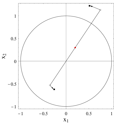
Figure 1: Image positions (square boxes) and critical line (full line) for a rotating SIS lens. The source is the grey circle. The centre of the coordinate-axes, the source and the two unperturbed images (empty boxes) lie on a straight line. Two images (filled boxes) are counter-clockwisely rotated, about the line of sight through the centre, with respect to this line. It is $L=10^{-3}$ and $r=50$.

Figure 2: The shift in the image positions (in units of arcsec) due to the gravito-magnetic field for source moving parallelly to the $y_{1}$-axis. Thick and thin lines are for $y_{2}=0.01$ and 0.1, respectively. Full and dashed lines refer to the two images. It is $L=4{\times}10^{-5}$ and $r=15$.

Figure 3: A source (the grey circle) inside the central caustic of a rotating SIS is multiple imaged in a cross shaped pattern; the four filled box locate the four images. The critical line is also plotted. It is $r=15$ and $L=3.5{\times}10^{-5}$.

In general, the inversion of the lens equation is a mathematical demanding problem. However, since the gravito-magnetic effect in the weak field limit is an higher-order correction, a rotating system can be studied in some details using a perturbative approach (Sereno, 2003a). The lens equation can be expressed in a dimensionless form as

$${\bf y}={\bf x}-\mbox{\boldmath$\alpha$}({\bf x}).$$ (28)

The unperturbed images are solutions of the lens equation for $L=0$. When $y\equiv|{\bf y}|<1$, a static SIS lens produces two images, collinear with the source position and the lens centre, at radii $x=y+1$ and $x=y-1$. When $y>1$, only one image forms, at $x=y+1$.

Under the condition $L\ll 1$, we can obtain approximate solutions to the first-order in $L$, given by

$${\bf x}\simeq{\bf x}_{(0)}+L{\bf x}_{(1)},$$ (29)

where ${\bf x}_{(0)}$ and ${\bf x}_{(1)}$ denote the zeroth-order solution (i.e. the solution of the lens equation for $L=0$), and the correction to the first-order, respectively. By substituting equation (29) in the vectorial lens equation, equation (28), we obtain the first-order perturbations,

$$x_{(1)1} = x_{(0)}^{2}+\left(\frac{3}{2}r-2x_{(0)}+x_{(0)}^{2}\right)\frac{x_{(0)1}^{2}-x_{(0)}^{3}}{x_{(0)}^{2}(x_{(0)}-1)},$$ (30)

$$x_{(1)2} = \left(\frac{3}{2}r-2x_{(0)}+x_{(0)}^{2}\right)\frac{x_{(0)1}x_{(0)2}}{x_{(0)}^{2}(x_{(0)}-1)}.$$ (31)

For a source on the $y_{1}$-axis ($y_{2}=0$), equations (30) and (31) reduce to

$$x_{(1)1} = -\frac{3}{2}r+2|x_{(0)1}|$$ (32)

$$x_{(1)2} = 0.$$ (33)

When $L>0$, photons with an impact parameter $x_{1}<0$ ($x_{1}>0$) go around the lens in the same (opposite) sense of the deflector. Due to the contribution to the deflection angle from the mass outside the impact parameter, photons which impact the lens plane on the $x_{1}$-axis at $x_{1}>0$ move closer to the centre. This feature, which is peculiar of light rays propagating inside a halo, is opposite to the case of propagation outside a spinning sphere (Sereno, 2003a), when photons in the equatorial plane moving in the same (opposite) sense of rotation of a deflector form closer (farther) images with respect to the non-rotating case. In fact, in the last case, there is no mass outside the photon path. If we do not limit to the equatorial plane, for $L>0$, the images are rotated counter-clockwisely around the line of sight with respect to the static case, see Fig. 1.

Let us consider the gravito-magnetic correction to the deflection angle for a typical galaxy lens at $z_{\rm d}=0.3$ with $\sigma_{\rm v}\sim 250$ Km s^-1, $R_{\mathrm{SIS}}\stackrel{{\scriptstyle<}}{{\sim}}100$ Kpc and $\lambda\sim 0.1$, and a background quasar at $z_{\rm s}=2.0$. Such a configuration correspond to $L\sim(2-4){\times}10^{-5}$ and $r\simeq 15$. For some particular source positions, the shift in the image positions in the lens plane with respect to the static case can be as large as $0.1\arcsec$. In Fig. 2, we plot the shift in the image positions for a source moving along the $y_{1}$-axis, i.e for $y_{2}=const.$ The maximum variation occurs when the source nearly crosses the projected rotation axis.

The critical curve is slightly distorted. The solution of $\det A(x_{1},x_{2})=0$, with respect to $x_{2}$, is

$$x_{2}(x_{1})\simeq\pm\left\{\sqrt{1-x_{1}^{2}}+\frac{x_{1}}{\sqrt{1-x_{1}^{2}}}L\right\}.$$ (34)

The area of the critical curve slightly grows and its centre shifts of $L$ along the $x_{1}$-axis. The critical curve intersects the $x_{1}$-axis in $x_{1}\simeq L{\pm}1$. The changes in the width and in the height of the critical curve are of order ${\cal O}(L^{2})$.

The four extremal points of the critical curve can be mapped onto the source plane through the lens equation to locate the cusps of the caustic. We find a diamond-shaped caustic with four cusps, centred in $\left\{y_{1},y_{2}\right\}=\left\{L(\frac{3}{2}r-1),0\right\}$. The axes, of semi-width $\sim L^{2}$, are parallel to the coordinate axes. The orientation and the position on the caustic depends on both the strength and orientation of the angular momentum and on the radius of the lens. When the source is inside the caustic, two additional images form. Since the axial symmetry is broken by the gravito-magnetic field, the Einstein ring is no more produced. A source, which is inside the central caustic, is imaged in a cross pattern, see Fig. 3.

6 Time delay

Figure 4: The gravito-magnetic time delay (in units of days) for a source moving parallelly to the $y_{1}$-axis. Thick and thin lines are for $y_{2}=0.01$ and 0.1, respectively. It is $L=4{\times}10^{-5}$ and $r=15$.

As we have seen in Section 2, the time delay for a spinning SIS is made of three main contributions: the geometrical time delay, $\Delta t_{\rm geom}$, the unperturbed gravitational time delay by a static SIS, $\Delta t_{\rm 0}$, and, finally, the gravito-magnetic time delay, $\Delta t_{\mathrm{GRM}}$,

$$\Delta t\simeq\Delta t_{\rm geom}+\Delta t_{0}+\Delta t_{\mathrm{GRM}}.$$ (35)

The main contribution to the gravitational time delay of a light ray with respect to the unperturbed path can be re-written as

$$c\Delta t_{0}=4\pi(1+z_{\mathrm{d}})D_{\rm d}\left(\frac{\sigma_{\mathrm{v}}}{c}\right)^{2}\theta,$$ (36)

where $\theta$ is the modulus of the angular position in the lens plane, $\mbox{\boldmath$\theta$}=\mbox{\boldmath$\xi$}/D_{\mathrm{d}}$. The gravito-magnetic time delay is

$$c\Delta t_{\rm GRM} \simeq -24\pi\left(\frac{\sigma_{\mathrm{v}}}{c}\right)^{3}(1+z_{\mathrm{d}})D_{\rm d}\left(\frac{3}{2}-\frac{\theta}{\theta_{\mathrm{SIS}}}\right)\theta_{1}\lambda$$ (37)

$$\simeq -36\pi\left(\frac{\sigma_{\mathrm{v}}}{c}\right)^{3}(1+z_{\rm d})D_{\rm d}\theta_{1}\lambda$$ (38)

where $\theta_{1}$ is the angular distance of an image from the projected rotation axis and $\theta_{\mathrm{SIS}}\equiv R_{\mathrm{SIS}}/D_{\mathrm{d}}$. To obtain equation (38), we have used the relation $x\ll r$. An approximate relation holds between $\Delta t_{0}$ and the gravito-magnetic time delay,

$$\Delta t_{\mathrm{GRM}}\simeq-9\cos\vartheta\left(\frac{\sigma_{\mathrm{v}}}{c}\right)\lambda\Delta t_{0}.$$ (39)

Since $L\ll 1$, the angular separation between the two images is nearly

$$\Delta\theta\simeq 8\pi\left(\frac{\sigma_{\mathrm{v}}}{c}\right)^{2}\frac{D_{\rm ds}}{D_{\rm s}},$$ (40)

and the gravito-magnetic induced retardation between the two images, $\Delta T_{\mathrm{GRM}}\equiv\Delta t_{\mathrm{GRM}}({\bf x}_{a})-\Delta t_{\mathrm{GRM}}({\bf x}_{b})$, can be approximated as

$$c\Delta T_{\rm GRM}\simeq 288\pi^{2}\cos\vartheta\frac{D_{\rm ds}D_{\rm d}}{D_{\rm s}}\left(\frac{\sigma_{\mathrm{v}}}{c}\right)^{5}\lambda.$$ (41)

Since the two images are nearly collinear with the lens centre, the gravito-magnetic time delay is nearly independent of the cut-off radius.

For a typical lensing galaxy at $z_{\rm d}=0.5$ with $\sigma_{\mathrm{v}}\sim 250$ Km s^-1, and a background source at $z_{\rm s}=2.0$, the gravito-magnetic time delay is $\sim 0.1-0.2$ days for $\lambda\sim 0.05$-0.1. In Fig. 4, the time delay between the images is plotted as a function of the source position for a source moving perpendicularly to the projected rotation axis. The distance of the source from the $y_{1}$-axis determines the width of the transition between the extremal values.

6.1 The Hubble constant

Figure 5: Relative error in the estimate of the Hubble constant, due to neglecting the gravito-magnetic field, for a source moving with fixed $y_{2}=0.1$. It is $L=2.5{\times}10^{-3}$ and $r=15$.

Any gravitational lensing system can be used to determine the Hubble constant (Refsdal, 1964). Neglecting the gravito-magnetic correction can induce an error in the estimate of the Hubble constant. In general, it is

$$H_{0}\Delta t={\cal F}(\sigma_{\mathrm{v}},...,z_{\rm d},z_{\rm s};\Omega_{i0}),$$ (42)

where the dimensionless function ${\cal F}$ depends on the lens parameters and on the cosmological density parameters, but the latter dependence is not very strong. A lens model which reproduces the positions and magnifications of the images provides an estimate of the scaled time delay $H_{0}\Delta t$ between the images. Therefore, a measurement of $\Delta t$ will yield the Hubble constant. Let us consider a rotating galaxy, described by a SIS with known dispersion velocity and redshift, which forms multiple images of a background quasar at redshift $z_{\rm s}$. An observer can measure the time delay between the two images, $\Delta T_{\mathrm{obs}}$, and their positions, ${\bf x}_{a}$ and ${\bf x}_{b}$. The unknown source position ${\bf y}$ can be obtained by inverting the lens equation. In terms of the dimensionless Fermat potential $\phi$, the measured Hubble constant turns out to be

$$H_{0}=\frac{1}{\Delta T_{\mathrm{obs}}}F(z_{\rm d},z_{\rm s},\sigma_{\mathrm{v}})|\phi({\bf x}_{a},{\bf y})-\phi({\bf x}_{b},{\bf y})|,$$ (43)

where

$$F(z_{\rm d},z_{\rm s},\sigma_{\mathrm{v}})\equiv(1+z_{\rm d})\left[4\pi\left(\frac{\sigma_{\mathrm{v}}}{c}\right)^{2}\right]^{2}\frac{r_{\rm d}r_{\rm ds}}{r_{\rm s}}$$ (44)

and $r$ is the angular diameter distance in units of $c/H_{0}$.

If, we assume a static lens model to model the data, the estimated Hubble constant is

$$H_{0}^{\mathrm{ST}}=\frac{1}{\Delta T_{\mathrm{obs}}}F(z_{\rm d},z_{\rm s},\sigma_{\mathrm{v}})2y^{\mathrm{ST}}.$$ (45)

where the “not correct” estimated position of the source is

$${\bf y}^{\rm ST}=\frac{1}{2}\left\{\sum_{a,b}{\bf x}_{i}-\frac{{\bf x}_{i}}{|{\bf x}_{i}|}\right\}.$$ (46)

The relative error in the determination of the Hubble constant is

$$\frac{\Delta H_{0}}{H_{0}}=\frac{2y^{\rm ST}-|\phi({\bf x}_{a},{\bf y})-\phi({\bf x}_{b},{\bf y})|}{|\phi({\bf x}_{a},{\bf y})-\phi({\bf x}_{b},{\bf y})|};$$ (47)

For a source at fixed $y_{2}$, the maximum error is $\sim 1/2\left|L/y_{2}\right|$, see Fig. 5. Since usually $L\stackrel{{\scriptstyle<}}{{\sim}}10^{-4}$, the induced relative error is really negligible.

7 Discussion

Since the physics of gravitational lensing is well understood, the gravito-magnetic time delay may provide a new observable for the determination of the total mass and angular momentum of the lensing body (Ciufolini & Ricci, 2003). Although a detailed model may be required to reproduce the overall mass distribution in the lens, interpretation of time delay is based on a limited number of parameters. Provided the cluster where the deflector lies can be described by a simple expansion, the only parameters needed to model the time delay are those needed to vary the average surface density of the lens near the images and to change the ratio between the quadrupole moment of the lens and the environment (Kochanek & Schechter, 2004). Furthermore, the presence of an observed Einstein ring can provide strong independent constraints on the mass distribution.

We have developed our treatment of the gravito-magnetic time delay by modeling the lens as a SIS. Isothermal models are supported by both theoretical prejudices and estimates from observations of early-type galaxies so that SIS turns out to be a surprisingly realistic starting point for modeling lens potentials. Gravito-magnetic time delays of $\sim 0.1$-0.2 days can be produced in typical lensing systems. A broad range of methods for reliably determining time delays from typical data and a deep understanding of the systematic problems has been developed in last years. Time delay estimates are more and more accurate and an accuracy of 0.2 days has been already obtained in the case of B0218+357 (Biggs et al., 1999), so that the detection of the gravito-magnetic time delay will be soon within astronomers’ reach. Observations with radio interferometers or $HST$ can measure the relative positions of the images and lenses to accuracies $\stackrel{{\scriptstyle<}}{{\sim}}0.005\arcsec$. Shifts in the image positions due to a gravito-magnetic field are usually well above this limit.

Our results are nearly unaffected by the presence of low-mass satellites and stars. These substructures do not have any impact on time delays and can only produce random perturbations of approximately $0.001\arcsec$ in image positions (Kochanek & Schechter, 2004), quite below the gravito-magnetic effect. Deviations from circular symmetry due to either the ellipticity of the deflector or the local tidal gravity field from nearby objects should be considered too. However, for a singular isothermal model with arbitrary structure, the time delays turn out of be independent of the angular structure (Kochanek & Schechter, 2004). Other higher-order effects, such as the delay due to the quadrupole moment of the deflector, should be considered in addition to the gravito-magnetic time delay. Unlike other effects, a gravito-magnetic field can break the circular symmetry of the lens, inducing characteristic features in lensing events (Sereno, 2003b). At least in principle and for some configurations of the images, a suitable combinations of the observable quantities can be used to remove additional effects, due to a quadrupole moment, from observational data (Ciufolini & Ricci, 2002; Ciufolini et al., 2003). Furthermore, when the lensed images lie on opposite sides of the lens galaxy, the time delay becomes nearly insensitive to the quadrupole structure of the deflector (Kochanek & Schechter, 2004).

Measurements of gravito-magnetic time delays could offer an interesting prospective to address the “angular momentum problem”. Cold dark matter models of universe with a substantial cosmological constant appear to fit large scale structure observations well, but some areas of possible disagreement between theory and observations still persist. The most serious small scale problem regards the origin and angular momentum in galaxies (Primack, 2004). Two “angular momentum problems” prevent the formation of realistic spiral galaxies in numerical simulations (Primack, 2004): i) overcooling in merging satellites with too much transfer of angular momentum to the dark halo and ii) the wrong distribution of specific angular momentum in halos, if the baryonic material has the same angular momentum distribution as dark matter halo. Detection of gravito-magnetic effects in gravitational lensing systems due to the spin of the deflector, either through time-delays measurements, as discussed in this paper, or through observations of the rotation of the plane of polarization of light waves from the background source (Sereno, 2004), could provide direct estimates of angular momentum and help in developing a better understanding of astrophysics in galaxies.

References

- Biggs et al. (1999) Biggs A. D., Browne I. W. A., Helbig P., Koopmans L. V. E. e. a., 1999, MNRAS, 304, 349
- Capozziello et al. (2003) Capozziello S., Cardone V. F., Re V., Sereno M., 2003, MNRAS, 343, 360
- Capozziello & Re (2001) Capozziello S., Re V., 2001, Phys. Lett. A, 290, 115
- Ciufolini et al. (2003) Ciufolini I., Kopeikin S., Mashhoon B., Ricci F., 2003, Phys. Lett. A, 308, 101
- Ciufolini & Pavlis (1998) Ciufolini I., Pavlis E., 1998, Science, 279, 2100
- Ciufolini & Pavlis (2004) Ciufolini I., Pavlis E., 2004, Nat., 431, 958
- Ciufolini & Ricci (2002) Ciufolini I., Ricci F., 2002, Class. Quantum. Grav., 19, 3863
- Ciufolini & Ricci (2003) Ciufolini I., Ricci F., 2003, gr-qc/0301030
- Ciufolini & Wheeler (1995) Ciufolini I., Wheeler J., 1995, Gravitation and inertia. (Princeton University Press, Princeton)
- Dymnikova (1986) Dymnikova I. G., 1986, in IAU Symp. 114: Relativity in Celestial Mechanics and Astrometry. High Precision Dynamical Theories and Observational Verifications Gravitational time delay of signals in the Kerr metric. pp 411–416
- Fomalont & Kopeikin (2003) Fomalont E. B., Kopeikin S. M., 2003, ApJ, 598, 704
- Glicenstein (1999) Glicenstein J. F., 1999, A&A, 343, 1025
- Kochanek & Schechter (2004) Kochanek C. S., Schechter P. L., 2004, in Measuring and Modeling the Universe The Hubble Constant from Gravitational Lens Time Delays. p. 117
- Kopeikin (1997) Kopeikin S., 1997, J. Math. Phys., 38, 2587
- Kopeikin (2004) Kopeikin S., 2004, Class. Quantum Grav., 21, 3251
- Kopeikin & Mashhoon (2002) Kopeikin S., Mashhoon B., 2002, Phys. Rev. D, 65, 064025
- Kopeikin & Schäfer (1999) Kopeikin S. M., Schäfer G., 1999, Phys. Rev. D, 60, 124002
- Mo et al. (1998) Mo H. J., Mao S., White S. D. M., 1998, MNRAS, 295, 319
- Padmanabhan (2002) Padmanabhan T., 2002, Theoretical Astrophysics, Vol. III. Cambridge University Press, Cambridge
- Petters et al. (2001) Petters A. O., Levine H., Wambsganss J., 2001, Singularity theory and gravitational lensing. Birkhäuser, Boston
- Primack (2004) Primack J. R., 2004, in IAU Symposium The Origin and Distribution of Angular Momentum in Galaxies. p. 467
- Refsdal (1964) Refsdal S., 1964, MNRAS, 128, 307
- Schneider et al. (1992) Schneider P., Ehlers J., Falco E. E., 1992, Gravitational Lenses. (Springer-Verlag, Berlin)
- Sereno (2002) Sereno M., 2002, Phys. Lett. A, 305, 7
- Sereno (2003a) Sereno M., 2003a, MNRAS, 344, 942
- Sereno (2003b) Sereno M., 2003b, Phys. Rev. D, 67, 064007
- Sereno (2004) Sereno M., 2004, MNRAS, in press; astro-ph/0410015
- Sereno & Cardone (2002) Sereno M., Cardone V. F., 2002, A&A, 396, 393
- Vitvitska et al. (2002) Vitvitska M., Klypin A. A., Kravtsov A. V., Wechsler R. H. e. a., 2002, ApJ, 581, 799
- Weinberg (1972) Weinberg S., 1972, Gravitation and cosmology. Wiley, New York